
Abstract
This article presents a methodology that provides a continuous assessment of predictive maintenance (PdM) technologies with respect to specific business scenarios. The methodology integrates existing reliability and maintenance business analysis techniques and standards. The positive impacts that may have implementing these technologies have always been in mind. A critical simulation step is also added where different predictive maintenance strategies are simulated in order to obtain the optimal maintenance strategy. This Monte Carlo simulation relies on the reliability information based on the probability density distribution of failure for the system or component, providing as a result the optimal strategy among the proposed options. The article finally explains how this methodology has a positive impact not only on the cost-effectiveness of maintenance processes, but also on the maintenance information available.
Introduction
Performance improvements in the maintenance and conservation activities of physical assets are measured by availability and operational reliability. They should be obtained preserving maximum quality and safety levels and minimizing the costs. In the current scenario of competitiveness, improvement efforts are essential to reach high levels of effectiveness and efficiency in every company’s production or operational department. The purpose is to achieve competitive advantage (in products or offered services) based on different hard-to-copy aspects, that is, know-how.
To obtain maximum performance, the organizations must be prepared for changes, and there are three interconnected areas in the change concept: 1
Processes and workflows to achieve the improvements (e.g. doing more preventive work instead of corrective work, etc.).
Technologies to facilitate or enable some processes.
Organization and people within the organization must validate any change, so there is a need of tools to ease changes.
One of the approaches for improvement is to identify and to apply predictive maintenance (PdM) techniques and tactics which would help to identify anomalies with high reliability. In this context, PdM is still an important area of improvement for Original Equipment Manufacturers (OEMs), maximizing the value of their products through extended lifetime services, not just within warranty periods, as well as for end users –maximizing the availability and performance of their assets with optimum maintenance costs.
Usual PdM systems are mostly centred in just condition monitoring; that is, the identification of anomalies in order to mitigate critical system failures before time-based replacement (or repair) is completed. A typical feature is modelling the degradation process, using the condition monitoring data to estimate the remaining useful life and making maintenance decisions. 2 This is the usual approach at systems that require extra safety approaches (e.g. nuclear, aerospace). However, the true potential of PdM is related to the extension (or cancellation) of repair and replacement periods, helping companies in their shift from ‘fail and fix’ policies to ‘predict and prevent’. 3
There are different ways to achieve cost-effective PdM for physical assets. One vector of improvement is the use of high-tech elements which can serve to help maintenance specialists in rapid on-site inspections, or even to perform an online remote assessment of the asset conditions. Another vector is to rely on third-party services that can perform specialized analysis, diagnostics and audits over specific areas (e.g. the lubrication process).
The maintenance information gap
The positive effect of PdM approaches in the improvement of operation and maintenance processes may be mitigated by different reasons. The lack of adequate information concerning the maintenance process is one of them. The lack of information can be due to different causes. Several examples are as follows:
The signal is acquired (e.g. vibrations) but stored just locally due to difficulties in or cost of data transmission (e.g. wind turbines).
Usually the failures and work order handled by the maintenance personnel do not feed the OEM in order to understand the machinery reliability – different departments and even different companies.
Lack of information transmission between operation and maintenance processes, apart from scheduled plans for preventive maintenance and inspection. No information on machinery performance, nor on short-/medium-term operational schedule.
Condition signal acquired by third-party services (e.g. vibration, lubrication, thermography) and handled in isolation, with a single ‘condition monitoring’ purpose.
At the end, there is a lack of proper acquisition, transmission and storage of vital data that need to be shared and communicated with the appropriate areas of the company (management, operation, maintenance, OEM). It may be argued that this lack of the information systems is because of the organizational culture and business processes. However, in many cases, the opposite may be happening: the lack of adequate information channels is motivating a certain culture of isolation.
This is critical and has at least two different effects on the development of any strategy for continuous improvement:
At the starting point for any improvement, the quantity and quality of information that optimization of maintenance strategies may need can be discouraging. Simulation tools can help in identifying how a new PdM approach may help – or hinder – in the cost-benefit of the life cycle of the product or global productivity of the plant. But most of them rely on several types of data not available at the beginning.
During the whole process, there is a need for metrics. The identification of true improvements is also difficult if only partial information is available. The key performance indicators (KPIs) initially planned can become unreachable.
Existing approaches to cost-effectiveness analysis
Various methodological frameworks and models deal with the identification, comparison and improvement in maintenance policies. For example, Al-Najjar and Alsyouf 4 study the criteria for comparing the maintenance approach, and it proposes an evaluation methodology for identifying the most informative by means of fuzzy multiple-criteria decision-making. Márquez et al. 5 defined a process for maintenance management classifying maintenance engineering techniques, introducing a methodological framework in eight steps.
The importance of a cost-effectiveness analysis is key because it is the way to indicate if any profit or competitive advantage can be achieved by using more automatic maintenance tasks, especially PdM.
This analysis is usually done with a maintenance strategies simulator,6,7 which introduces the details related to predictive systems (sensor costs, inspection costs, estimations/probability of errors – false positives) with other data or information related to corrective and preventive maintenance costs and reliability information. 8
For instance, Berdinyazov et al. 9 presented a model for simulating improvements in maintenance. Their model begins with assigning each possible failure mode to one of three maintenance policies (i.e. corrective maintenance, periodic maintenance and condition-based maintenance). Then it simulates the cost associated with each failure mode and policy by means of Monte Carlo analysis. And finally, the contribution of all failure modes is added for obtaining the total maintenance cost.
Exakt is a software package by Optimal Maintenance Decisions Inc. for predicting and optimizing condition-based maintenance in order to improve reliability, reduce failures and save maintenance costs. It works by correlating measurable condition variables with failure modes and, as such, requires inputs such as event and condition data.
Feldman et al. 10 focus on an analysis of the costs associated with predictive, prognostic maintenance as compared to unscheduled maintenance. Discrete event simulation, implemented as a Monte Carlo analysis, is used for comparing various use cases with respect to the baseline unscheduled maintenance. Asadzadeh and Azadeh 11 have dealt with the importance of human and organizational aspects in optimization of condition-based maintenance.
Wang 12 uses bearing vibration to estimate the component condition and residual life. On top of the estimation of the component’s life, costs are added in order to support the decision process on the optimal replacement time. Xiang et al. 13 modelled equipment deterioration with time to failure distributions. Weibull distribution is fitted to the time of first failure data. For estimating the Weibull distribution, instead of actual data, a simulation of an environment is performed with a Markov chain in order to generate the data. The cost-benefit of the condition-based maintenance policy is assessed via simulation including corrective, preventive and periodic inspection actions, or in other words, including both age-based and condition-based maintenance policies.
Scope and contents of the article
This article illustrates a methodology to overcome this information gap, which helps in starting to take decisions with little information and allows a progressive increase in confidence (from a statistical point of view as well concerning communication with management) which depends on the level of information collected.
Section ‘Improvement model’ explains the overall methodology for constantly improving maintenance activity focusing on reducing maintenance costs, in order to achieve an optimal maintenance strategy, mainly based on predictive technologies.
Finally, section ‘Asset management simulation’ concentrates on the core of improvement model, presenting an implementation of a maintenance strategy simulation based on the probability density distribution of failure for the selected system or component.
Improvement model
Maintenance should be a constantly improving activity, which enhances the quality of service and optimizes operating costs. Condition-based maintenance and predictive strategies based on cutting-edge technologies are arriving on the market, and their continuous cost reduction opens wide opportunities, helping the operation and maintenance personnel to perform tasks more effectively.
There are cost-effectiveness studies of the different types of strategies, but it is normally difficult to measure with these tools the impact of predictive strategies.9,10,12–16 To overcome this gap, a simple model was developed to solve the difficulty of showing how PdM could help in a cost-effective way. This model is based on the application of different existing tools (Balance Scorecard, Failure Modes Effects and Cause Analysis – FMECA, Preliminary Hazard Analysis – PHA, etc.), and it follows a six-step structure based on a Deming cycle to gradually improve each process or service adapted to maintenance needs.
The innovation of this improvement model compared to previous approaches is the generalized concept of PdM to include, besides on-line sensors, inspections and off-line laboratory analysis. Besides this, we have additionally developed a possible combination of strategies for the simulator. Furthermore, this simulator considers the possibility of having different probability for false positives and negatives as it works with accuracy.
The cycle is continuously fed with new information to achieve an optimal maintenance working way in a cost-effective manner and keeping in mind strategies that are based on predictive technologies. The steps are carried out in a cyclical manner as shown in Figure 1.
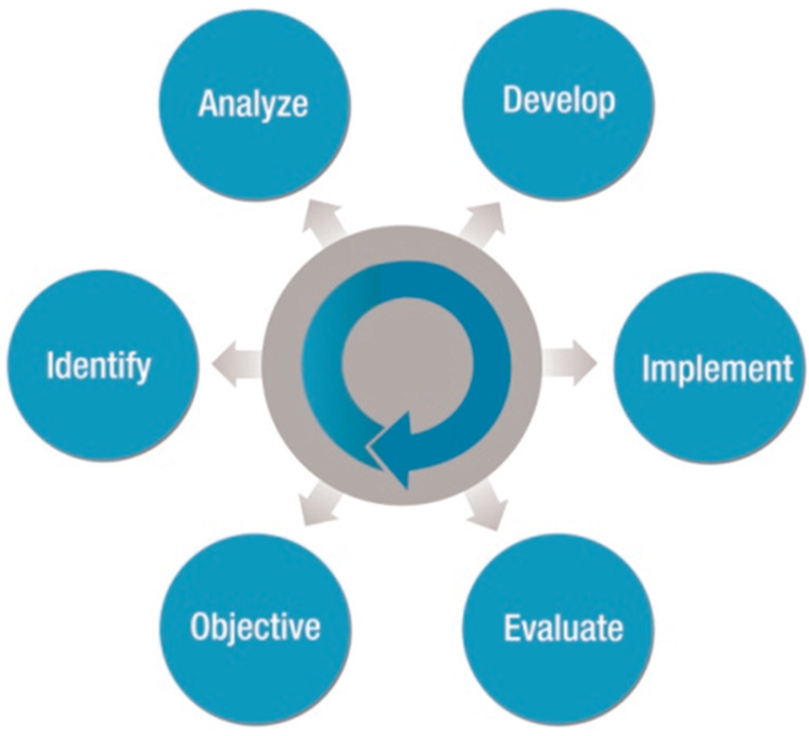
Deming cycle.
Selection of the objectives (step 1)
The first step is to establish the main objective. It is essential to know exactly the situation of the company in order to know what should be improved and to align the vision, mission, strategies, objectives and indicators. These objectives should be identified with KPIs with different approaches: financial, learning or technical. There are many different techniques that can serve to achieve the correct alignment between the company and indicators, such as Balanced Scorecard.
Identification of the most important products/processes (step 2)
The next step is the identification of the main objects or processes where the improvements are going to be critical with respect to their impact on the selected KPIs. The results include machinery parts (e.g. planetary systems), product types (e.g. specific wind turbine gearboxes) or target sectors (e.g. wind-farms with less than 50 MW) among others.
Criticality tables are used in order to rank the results and select an appropriate subset for further analysis and simulation in the next steps.
Analysis of the selected product/processes (step 3)
An exhaustive analysis of the selected products/processes is carried out to have a clear idea of their important aspects. Analysing the most critical assets is very useful in order to obtain the selected objectives, that is, the information of different tools: from Failure Mode and Effect Analysis (FMEA) to Risk Analysis (PHA) among others. A complete understanding of the assets identified in the previous step gives a better way to make improvements.
Identification of optimized asset management strategies for each critical product/processes (step 4)
This step consists of an analysis and an assessment of various maintenance strategies for the selected critical products/processes. There are a number of different techniques for implementing and analysing these aspects.
The cost assessment simulation is done in this step and is the most critical part of the whole model. An ad hoc optimization tool has been developed to better simulate the cost-effectiveness, and therefore this step will be further explained in this article.
The key issues in the simulation process are to use a valid source of information, to employ a relevant selection of key characteristics and behaviours, to make approximations and assumptions when necessary and to understand the fidelity and validity of the simulation outcomes. The simulation is developed by means of a Monte Carlo approach where the probability density distribution of failure for the equipment or component is estimated, first from bibliographical data and later from real failure information, increasing progressively the confidence value.
Implementation and assessment (steps 5 and 6)
These steps are run iteratively, in a separate cycle, in order to compare the simulation results in step 4 with the real results obtained after the deployment of the new strategies. This deployment is normally progressive (concept complete design, lab trials, first installs on selected machines, etc.).
The selected strategy is implemented at least in one control group in order to evaluate the results. New procedures, hardware and software technologies, will be deployed and tested. Using the initially defined KPIs, the assessment will evaluate whether the initial objectives have been fulfilled or not (Figure 2).
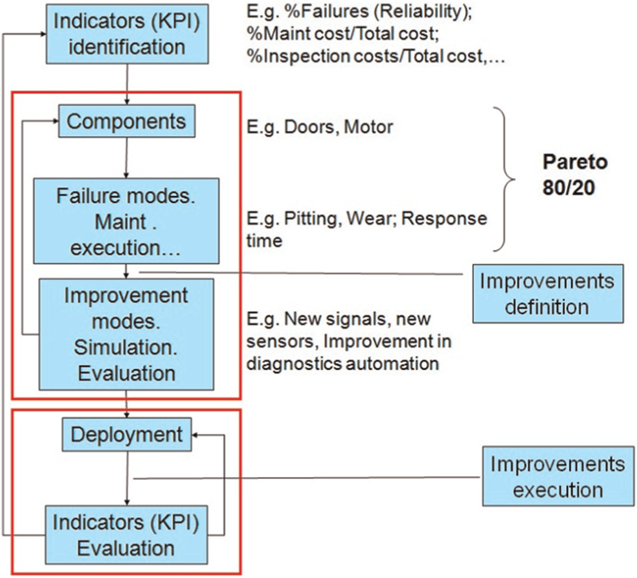
Deming cycle adapted for PdM strategies improvement.
If the objectives are not fulfilled, that is, there are large deviations from the simulated cost assessment, it is necessary to return back to the previous step and identify the deviations sources. If the objectives are being fulfilled, new objectives can be defined to follow with the continuous improvement programme, starting in this case a new cycle. The frequency of cycles is not pre-defined, and it depends on the information collected about objective fulfilment.
Asset management simulation
The reliability information on which the maintenance strategies simulator relies on is the probability density distribution of failure for the system or component. Such a function determines the possibility of a failure occurring at a given time. It is typically established from test or run-time data noticing the time at which failure occurs, also from calculated and/or existing reliability data.
The Weibull distribution is frequently employed because it is applicable to different phases in the life of a component or system (Figure 3). Weibull distribution is described by three parameters: scale (α), shape (β) and location (γ). The higher the scale value, the longer the life expectancy of a component. The shape factor distinguishes among early-type failures (β < 1), random-type failures as during useful life (β = 1) and wear-type failures (β > 1). In the first case (β < 1), failure rate decreases with time. It is constant for β = 1, and for β > 1, it increases with time. Finally, the location parameter affects the origin of the time axis and it usually is set to 0. Weibull distribution is flexible enough to model a variety of failure occurrence that are decreasing, increasing or constant, allowing it to describe any phase of a component’s lifetime.
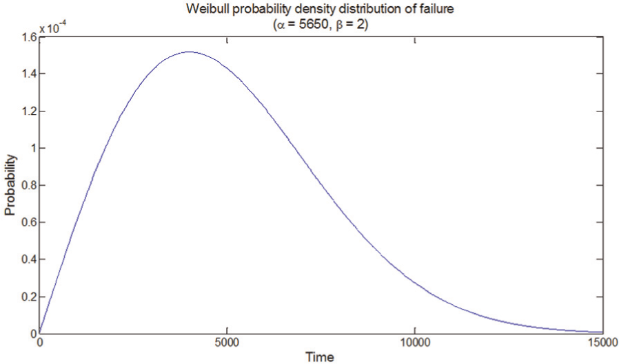
Example of Weibull probability density function.
Given this function, it is possible to apply Monte Carlo method for performing a random sampling and as a consequence for obtaining possible times at which failure occurs. A known way to do so is with the inverse of the cumulative Weibull distribution function, by means of performing a random sampling for it in order to obtain times of failure. As the process is repeated, the series of values obtained produce a more faithful description of the Weibull distribution.
With this methodology, it is possible to obtain a time of occurrence of a failure and, therefore, to anticipate the type and number of maintenance actions performed following a particular maintenance strategy and their result in terms of cost. This process is repeated for the Monte Carlo analysis to offer a faithful description, and time and costs accumulated. The cost per unit time is used in order to compare the results obtained with different maintenance strategies. In our approach, we have considered only Weibull distribution due to its flexibility, but any other failure distribution could be used in the simulation process if the degradation component model is known.
The following maintenance strategies have been considered for simulation:
Corrective. Maintenance actions are performed only when a failure occurs.
Preventive. Besides corrective maintenance actions, additional systematic maintenance actions are performed at every pre-defined time interval.
It is assumed that after corrective actions are performed, the time interval should be reset (as good as new), as it is often the case with, for example, oil replacement.
Inspection. Additional maintenance actions are performed based on the results of a failure detection analysis at every pre-defined time interval done by maintenance personnel.
Predictive. Maintenance actions performed based on the results of a failure detection analysis at every pre-defined time interval. In this case, the action is done by a laboratory (off-line) or technology integrated in the system/component (on-line).
Moreover, in a combined strategy, maintenance actions are performed according to the four aforementioned strategies. This is to say, besides corrective maintenance actions, systematic preventive maintenance is performed along with inspections and more frequent failure detection analyses.
Simulating a PdM strategy
The approach for simulating the application of a predictive strategy in maintenance involves establishing beforehand the error rate for the failure detection analysis. Typically, this error rate consists of a probability of false positives and a probability of false negatives. The former corresponds to the situation in which the analysis generates a false alarm; this is to say, the analysis detects a failure when it is actually not the case. The later corresponds to the opposite situation, in which the analysis does not detect a failure when it actually exists. The occurrence of false positives/negatives is simulated with a Monte Carlo analysis by means of a random sampling from a uniform distribution. If the value resulting from this random sampling is lower than the probability of false positives/negatives, the occurrence of a false positive/negative is indicated.
The approach for the PdM strategy simulation is a loop devised as follows. First, the Monte Carlo analysis on Weibull function provides the time at which the next failure is assumed to occur.
Next, the detection analyses until the last before failure or the end of useful life are checked. If any failure is a false alarm, then the process is stopped, the time of occurrence registered and the cost of the analyses performed is allocated to maintenance costs. Note that the last detection analysis before failure is not considered in this process because it is not affected by false alarms. The time registered (failure, false alarm or end of useful life) is accumulated as the usage time of the system.
If the accumulated time is equal to the end of useful life of the system, a replacement/refurbishment maintenance action is performed, with the assumption that the system will be as good as new afterwards. The cost of the action is allocated to maintenance costs.
If a false alarm has occurred, a repair maintenance action is performed and the cost allocated to maintenance costs. Note that maintenance costs will include the cost of the detection analyses as well, as explained above. If, otherwise, the last detection analysis before has been reached, it is checked whether it is a false negative, and if it is, a corrective maintenance action is performed, assuming the system will be as good as new afterwards. The cost of the action is allocated to maintenance costs, which include the cost of the detection analyses as well, as explained above.
Otherwise, this is to say that it is not a false negative; the detection analysis has succeeded in detecting a failure. A repair maintenance action is performed (assuming just before the instant of failure, thus making the most of the productive time, although in a real case, the prediction horizon may not be as exact or ample). The cost of the action is allocated to maintenance costs which include, as explained before, the cost of the detection analyses performed.
This procedure is repeated from the beginning until a production time and number of repetitions stipulated have been reached. Finally, as a result, the cost per time unit for the simulated maintenance strategy is calculated.
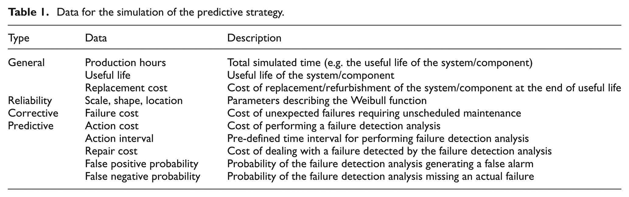
To sum up, Table 1 shows the data necessary for simulating the process.
Data for the simulation of the predictive strategy.
Given this process simulation for predictive strategy, the next step is to provide a decision support system to establish the optimal maintenance policy to be performed on the asset. This optimal policy is determined through the calculation of the following strategies, selecting the one which provides a minimum cost:
Corrective strategy.
Preventive strategy with optimal frequency of replacement task.
Predictive strategy with optimal frequency of inspections, sampling or measurement. In this case, different approaches could be considered.
As a result, the optimal strategy for the selected asset is provided according to the cost and reliability information provided.
Results and impact
Results with respect to existing models
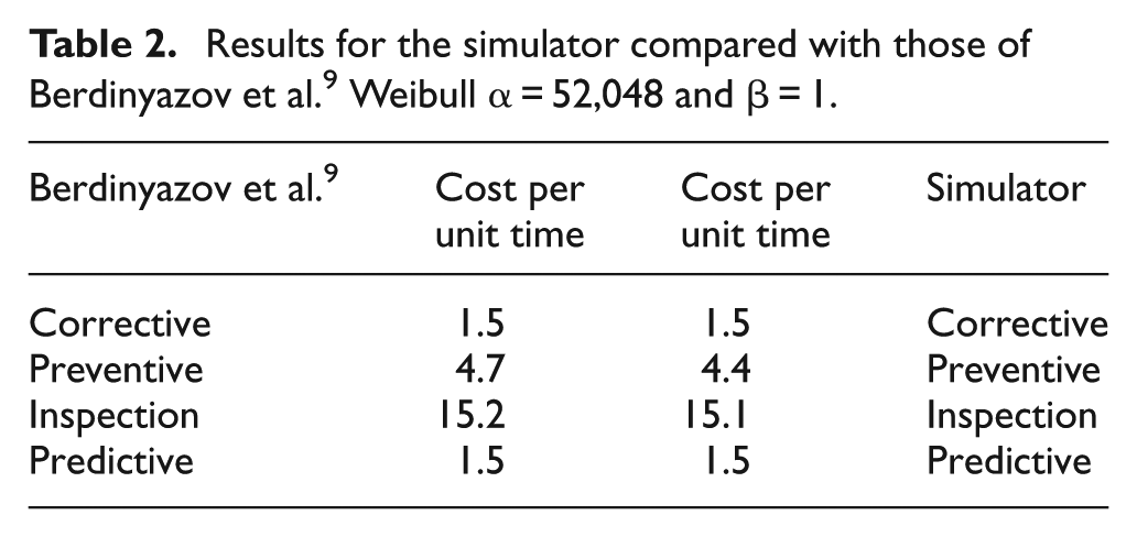
The developed simulator has been compared with an existing previous model. 9 This model is devised as a set of equations for calculating maintenance costs using similar data and reliability function with Monte Carlo analysis. However, the model works on the aggregated number of failures per period (e.g. preventive maintenance interval), whereas the simulator develops the appearance of failures in the maintenance process as time unfolds. With this simulation mechanism, we can introduce conditions, events, decisions or actions associated with a failure or between failures. For example, in the case of preventive maintenance strategy, it is assumed by the simulator that after corrective actions are performed, the systematic preventive time interval should be reset, as it is often the case with, for example, oil replacement. As shown in Table 2, this situation can be included in the simulator, and it results in economic savings in our case. In addition to this, Table 2 shows very similar results between the simulator and the model in corrective, inspection and predictive strategies, when using the same data. Notice that Berdinyazov et al. 9 do not consider the possibility of having different probability for false positives and negatives as it works with accuracy. We have also generalized the concept of PdM to include, besides on-line sensors, inspections and off-line laboratory analysis. Besides this, we have additionally developed the combined strategy for the simulator.
Results for the simulator compared with those of Berdinyazov et al. 9 Weibull α = 52,048 and β = 1.
Furthermore, Exakt tools make focus on calculating the optimal frequency for the preventive maintenance task through an accurate failure prediction as well as to support decision on perform maintenance replacement or not, always taking into account operating and condition variables. In this sense, the proposed simulation is complementary and proposes the optimal strategy to perform on the asset.
The improvement is being used to monitor several improvement cycles at this moment in many different systems, such as machine tools, windmill gearboxes or elevators. The initial reliability, KPIs and the main contributors to these KPI inefficiences are identified in step 1.). Step 2 (identification of the most important product/processes) focuses on different aspects of these systems, such as spindle, gear-box and door mechanism among others, as main contributors to such inefficiencies (in this case, there is a direct link with unreliability or number of failures).
Impact on improved OEM quality of services
Selecting these critical elements allows a detailed study of the principal failures and causes at step 3 (analysis of selected product/processes), using information of FMEA combined with information analysis of the machinery population.
The analysis of these products has been focused on technologies and processes with potential to identify the failure before it happened, and with the help of the work team knowledge, different systems were found to solve failures with different degrees of confidence and coverage of the different failure modes (e.g. a costly particle sensor can be much more accurate than a periodic inspection of the lubricant, but the degree of cost-effectiveness varies depending on the Mean Time Between failures – MTBF, the cost of the inspection and of the sensor, etc.).
The improvement analysis finishes with the estimation of the potential impact of the different strategies (corrective, time based and inspections) measured in Euros, comparing the maximum cost of the selected technologies and alternative strategies, considering several known or estimated variables such as frequency of the inspections, reliability, cost of failures, inspections and preventive actions. A typical representation can be seen in Figure 4.
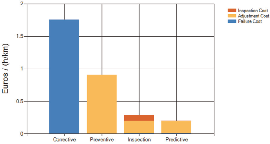
Impact of different strategies of maintenance of a mechatronic component within a system, taking into account a global KPI (cost) segmented at three different cost categories (cost of repair and loss of revenues when the component fails; cost of the preventive activities; and cost of the monitoring activities – whether remote or on-site).
These estimations allow different questions to be asked, such as,
What is the cost target for a sensor if we want to implement a remote monitoring system?
Which accuracy should have the sensor?
Which is the best inspection frequency if we prefer this option?
Which is more cost effective – corrective or preventive strategies?
In summary, this approach provides a framework to compare different strategies in a structured methodology, and simulation will be realistic depending on the supported reliability and cost information. For instance, reliability data could take into account potential hazards in the operational environment such as the use of equipment.
Impact on improved quality of information
Improvement cycle is not only focused on optimizing the maintenance processes, but it is also related to the process of information acquisition and storage as well as the identification of best indicators for finding deficiencies, which in other ways could be difficult to analyse.
First, the improvement of the information is very much related to the analysis of the first steps in the cycle. For instance, it is normal to notice a single indicator (usually related somehow to machinery reliability or availability) as initial KPI. During the project development, new indicators are discovered and these always carry specific actions to access new sources of information necessary to evaluate the indicators. This targeted search of specific information within the company, while running the improvement cycle, is much more rewarding than an initial global search of all the available information.
A typical increase in the number of indicators and associated KPIs are given in Table 3.
KPI evolution.
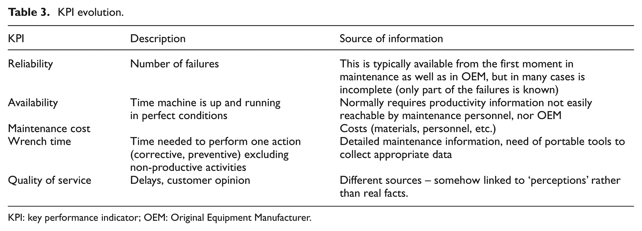
KPI: key performance indicator; OEM: Original Equipment Manufacturer.
On the other hand, the initial assessment with a reduced feedback expresses clearly the information lacks that the organization may have. For instance, an example may be to improve the way the failures are managed (e.g. to reduce the amount of incidences not yet linked with a clear type of failure). Vaguely defined fields of the work order may be erased (‘Other’ type of failures) when a clear and consolidated FMECA analysis is shared between engineering and maintenance areas. Clearer codes concerning failure, cause and action can be addressed through the initial improvement cycles.
Conclusion and further work
This article has presented how simulation tools can help identifying a new PdM approach in the cost-benefit of the product life cycle or plant productivity. This approach depends on several types of data probably not available at the beginning, and it has to be supported by a continuous improvement model also described in this article. The process of information acquisition and storage as well as the identification of best indicators are key for finding deficiencies, which in other ways could be difficult to analyse.
Furthermore, automating the continuous improvement, a previous step can be added where the simulation is performed from different ontologies containing information of the selected asset:
Structural information.
Failure modes and effects.
Costs during life cycle.
Detectability by sensing or inspections.
In this work, the Weibull distribution is calculated from a database that contains information on faults, at the component level, and the target would be to achieve the optimal strategy at failure model level, since adding sensors in predictive strategies would avoid some specific failure modes. Also, providing asset tree structure enables the simulation at different levels, having a new set combination to perform the selection of the most cost-effective maintenance strategy.
Footnotes
Declaration of conflicting interests
The author(s) declared no potential conflicts of interest with respect to the research, authorship, and/or publication of this article.
Funding
The author(s) received no financial support for the research, authorship, and/or publication of this article.