
Abstract
Little practical results are known about the cutting tool optimal replacement time, specifically for machining of composite materials. Due to the fact that tool failure represents about 20% of machine down-time, and due to the high cost of machining, in particular when the work piece’s material is very expensive, optimization of tool replacement time is thus fundamental. Finding the optimal replacement time has also positive impact on product quality in terms of dimensions and surface finish. In this article, two new contributions to research on tool replacement are introduced. First, tool replacement mathematical models are proposed. These models are used in order to find the optimal time to tool replacement when the tool is used under variable machining conditions, namely, the cutting speed and the feed rate. Proportional hazards models are used to find an optimal replacement function. Second, this model is obtained during turning titanium metal matrix composites. These composites are a new generation of materials which have proven to be viable in various industrial fields such as biomedical and aerospace, and they are very expensive. Experimental data are obtained and used in order to develop and to validate the proportional hazards models, which are then used to find the optimal replacement conditions.
Introduction
Titanium metal matrix composites (TiMMCs) inherit outstanding characteristics such as low weight, high mechanical and physical properties, high stiffness, and strength. For example, the density of conventional TiMMCs is 4040 kg/m3, and the stiffness is 200 GPa. 1 Although very expensive, metal matrix composites (MMCs) are a new generation of materials which have proven to be viable in various fields such as biomedical and aerospace industrial. Finding the optimal tool replacement time in machining TiMMCs is important in order to decrease the scrapped products and thus the cost of machining, and/or to increase the tool life, and thus to increase the availability of the cutting tool. Replacing the tool only at failure may leave undesired effects on the product’s quality characteristics, namely, the dimensions and the surface finish. This may lead to scrapping of the product. The poor tool condition may cause wastage of subsequent production resources and the loss of customer’s goodwill. 2 In general, the determination of the optimal replacement time is considered an important economic factor in machining. 3
The cutting tool cost represents around 25% of the total machining cost.4,5 The cutting tool failure represents about 20% of machine down-time, 6 and replacing cutting tool earlier or later than necessary will cause either loss of valuable resources or scrapping of products. 7 Moreover, the tool replacement policy is one of the important aspects of tool management. 8 For these reasons, finding the time at which the tool should be replaced is fundamental. Much research tried to improve tool life in several ways. For example, Klim et al. 3 proposed a method to improve cutting tool life in machining using the effect of feed variation on tool wear and tool life. By changing feed rate, the reliability function is changed, and thus the tool life is changed. The Weibull distribution was used to fit the data. The experiment was conducted under constant cutting speed. Balazinski and Mpako 9 proposed an improvement of tool life through using two discrete feed rates. The method depends on varying the feed rate throughout the cutting process. By varying the feed, the tool-chip contact area increases, the tool wear rate decreases, and consequently leads to improvement of the cutting tool life. The experiment was conducted under constant cutting speed. Lin and Shyu 10 concluded that using variable feed machining, and constant cutting speed, when drilling stainless steel is a significant method for improving the cutting tool life.
Other researches tried to find the optimal replacement strategy by using proportional hazards models (PHMs) for modeling tool life, then using another technique to find optimal strategy. For example, Mazzuchi and Soyer 11 used a PHM to assess machine tool reliability. Fully Bayesian analysis is used to find optimal machining conditions. Liu and Makis 12 derived a formula to calculate the cutting tool reliability under variable cutting conditions. They used PHMs while considering the machining conditions as covariates. Liu et al. 13 extended the work by developed algorithm based on stochastic dynamic programming for finding the optimal tool replacement times in a flexible manufacturing system. Ding and He 14 used a PHM by considering vibration signals as a time-dependent covariate. The author suggests that vibration signals are good indicators to tool wear. Reliability analysis based on feature extraction from tool vibration signals is introduced. They found remarkable relationship between the tool condition monitoring information and the life distribution of tool wear by using PHMs. Other research used classical Weibull distribution to fit tool life distribution. For example, Vagnorius et al. 15 used the Weibull distribution to fit tool life distribution. The optimal replacement time for metal cutting is determined from a total time on test (TTT) plot.
Some researchers tried to improve the cutting tool life by changing feed rates while the cutting speed is constant;3,9,10 others consider the PHM as good model for tool life representation.7,11,16 In most of these models, it was assumed that the machining conditions have significant effect over the entire tool life, but finding tool replacement models is still unavailable. The objective of this article is to find tool replacement optimization models which can be used in order to minimize the cost or to maximize the availability during turning TiMMCs under variable conditions. The PHM is used to model in order to find these models. The Cutting speed (
Model description of a tool operating in varying conditions
In 1907, Taylor
17
developed the classical relationship between tool life (
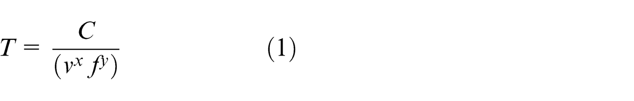
where
where
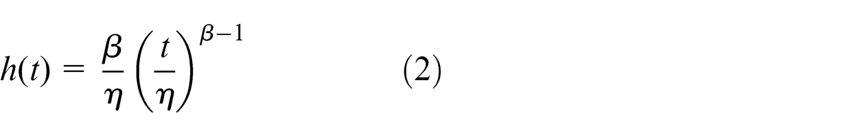
Using the Weibull model as a baseline function in modeling the tool failure was considered by Tail et al.
7
, Mazzuchi and Soyer,
11
and Makis
16
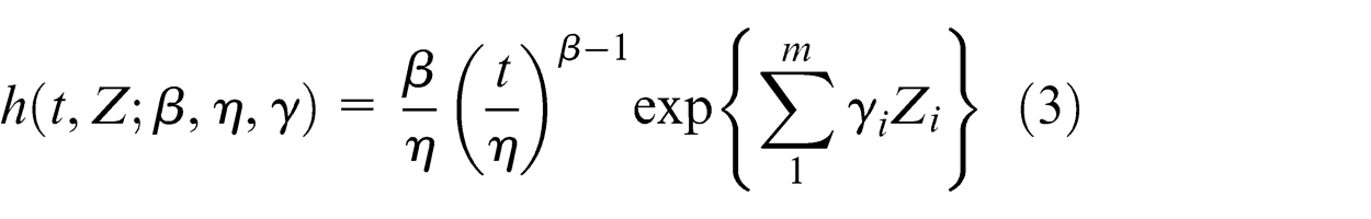
This model is sometimes called the Weibull parametric regression model. The covariates are the cutting speed (
In this article, we consider two states: the normal and the failure states. This latter is defined by the tool wear reaching a predefined level
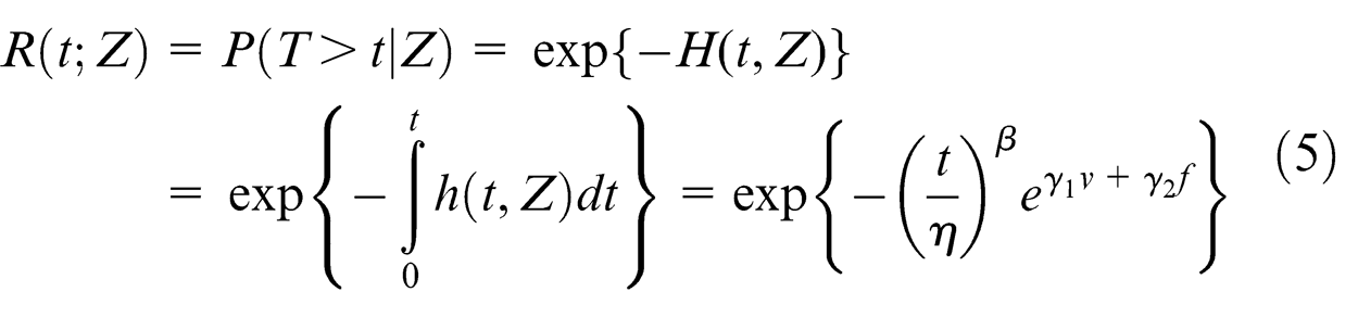
where
Optimal replacement policy
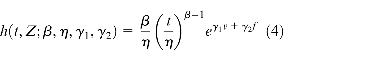
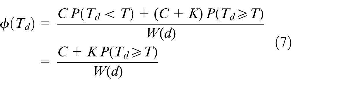
The classical age replacement strategy recommends replacement of the cutting tool at failure, that is, when the tool wear threshold is reached, or when it reaches a certain age which minimizes the cost per unit time. In the classical strategy, the effects of the covariates are not taken into account. In this article, the effects of the cutting speed (
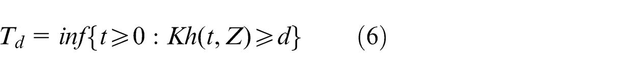
where
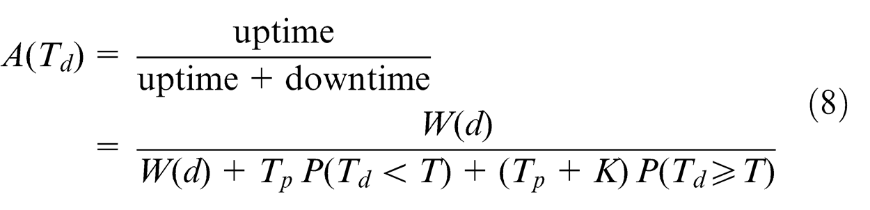
Similarly, we represent the availability function as in equation (8)
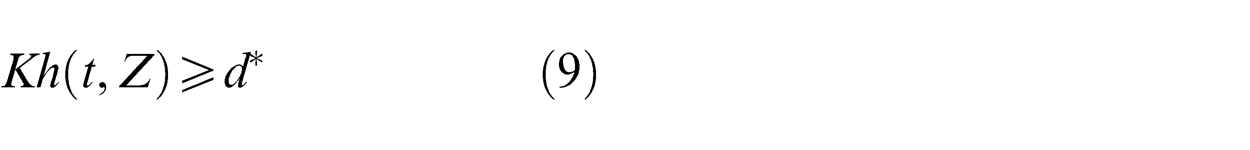
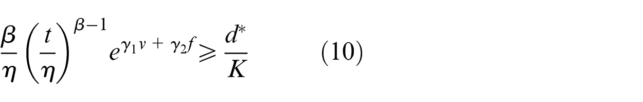
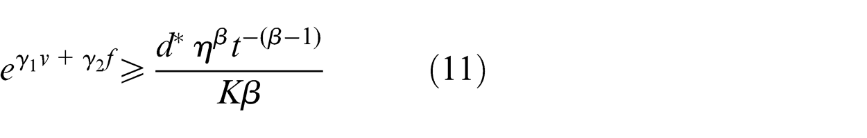
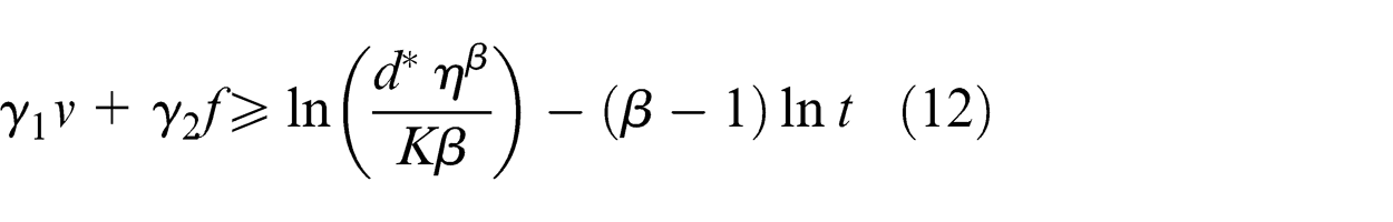
When
The objective is to find
Description of the experiment
Equipment: A 6-axis Boehringer NG 200, computer numerical control (CNC) turning center is used in order to conduct experiments, as shown in Figure 1. Tool material: TiSiN-TiAlN nano-laminate physical vapor deposition (PVD) coated grades (Seco TH1000 coated carbide grades) is used. Workpiece material: A cylindrical bar of Ti-6Al-4V alloy matrix reinforced with 10%−12% volume fraction of TiC ceramic particles is used. Experimental details: The experiments were conducted using full factorial designs with two factors, two levels (
The experimental setup.
The coded design of experiment.
The design of experiment.
The cutting tool fails when the tool becomes dull and no longer operates within acceptable quality.
5
The common way of quantifying the tool time to failure (TTF) is to put a limit on the maximum acceptable flank wear,
Figure 2 shows the wear interpolation procedure in order to calculate the TTF; the wear evolution between two measurements (
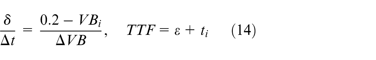
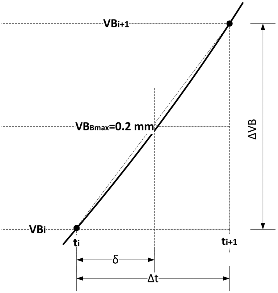
Wear interpolating.
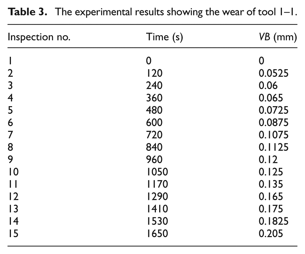
The experimental results showing the wear of tool 1–1.
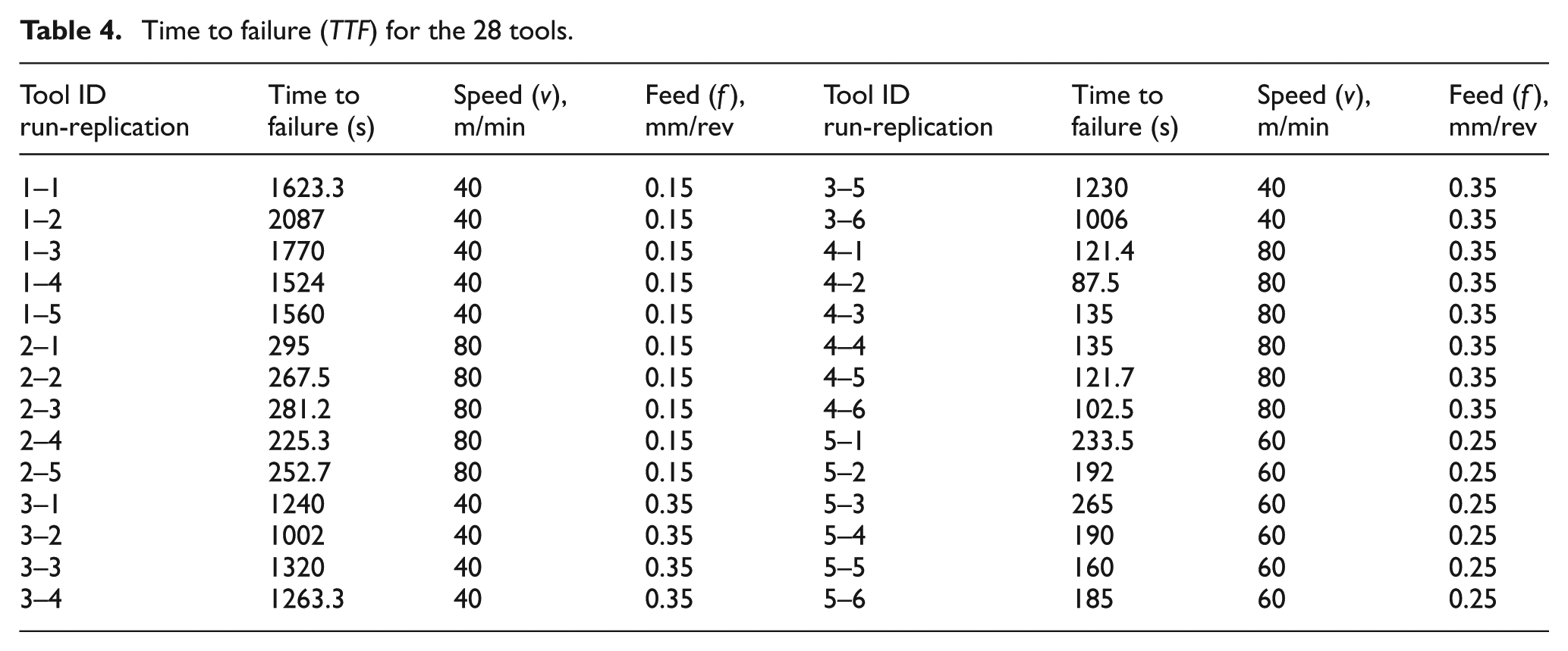
Time to failure (TTF) for the 28 tools.
Development of the model and results
The PHM parameters are estimated using EXAKT software. 18 The resulting hazard function is given as follows in equation (15)
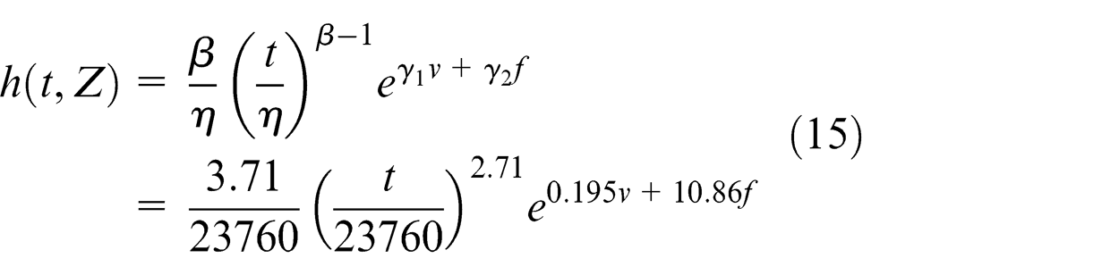
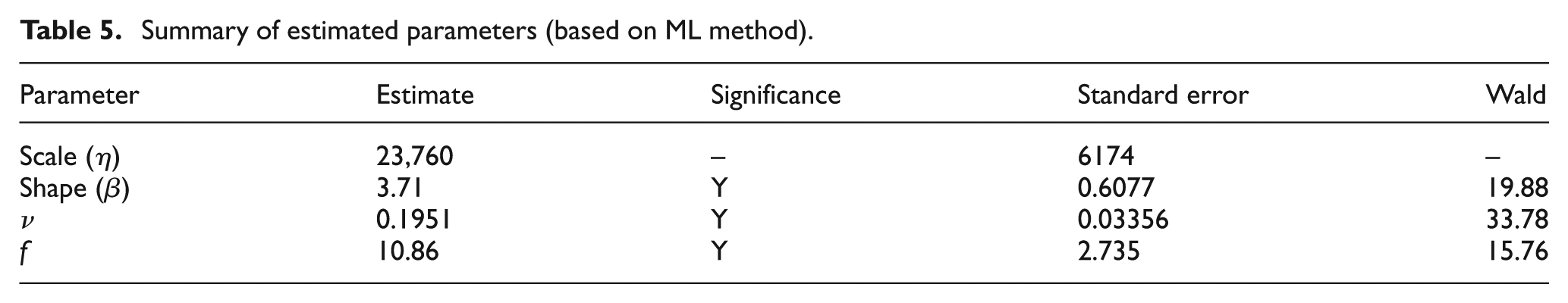
The covariate parameters
Summary of estimated parameters (based on ML method).
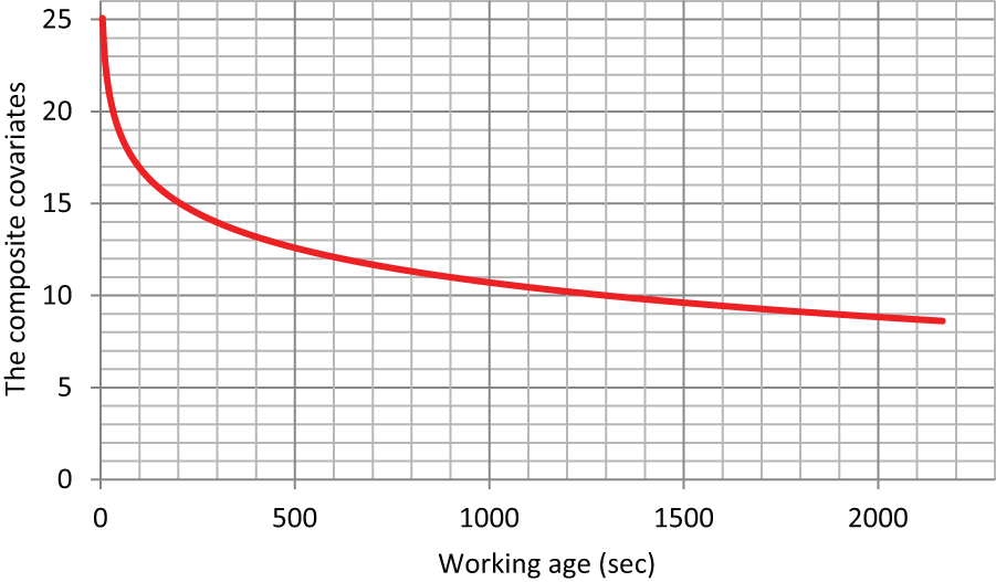
In order to know how the cutting speed and the feed rate affect the hazard rate, a simple normalization procedure is done. Since the cutting speed and the feed are in the range
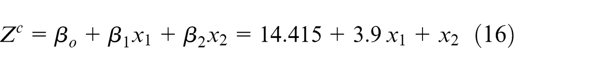
where
In order to validate the model, Kolmogorov–Smirnov test (K-S test) and logarithmic reliability function analysis are done. K-S test evaluates the model fit. The test checks the null hypothesis that the
Summary of goodness of fit test results.
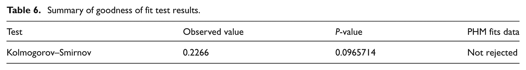
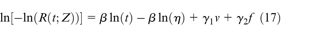
Figure 3 shows the analysis of the logarithmic reliability function (log minus log plot). 24 From equation (5), the linear equation for each run will be as follows
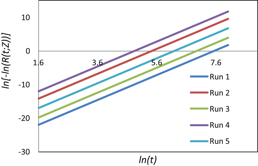
Logarithmic reliability function plot for each run.
The logarithmic reliability function in equation (17) is linear in
Based on equation (15), the failure rates are plotted for each run in Figure 4. The effect of machining conditions on the failure risk is clear when we compare between different runs. For example, by comparing between run 1 and run 2 which have the same feeds rates but different speeds, and also by comparing between run 2 and run 4 which have the same speeds but different feed rates, obviously, the effect of cutting speed is much higher than the effect of feed rate.
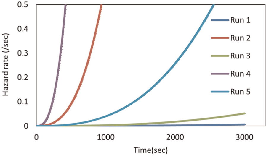
Hazard rate curves for each run.
After determining the PHM, the optimal replacement policy-cost analysis is performed. The optimal replacement function is calculated with a cost ratio r = 2 (preventive replacement cost is estimated to be $100, and the failure replacement cost is $200, thus K is equal to $100); r is the ratio of the failure replacement cost to preventive replacement cost, and it is calculated considering the tool and material cost; r is always more than 1 to make sense to maintain the tool preventively. As shown in Figure 5, the optimal time to replacement
Optimal replacement function-cost analysis.
Similarly, we find the optimal replacement function that maximizes the availability. The optimal time to replacement
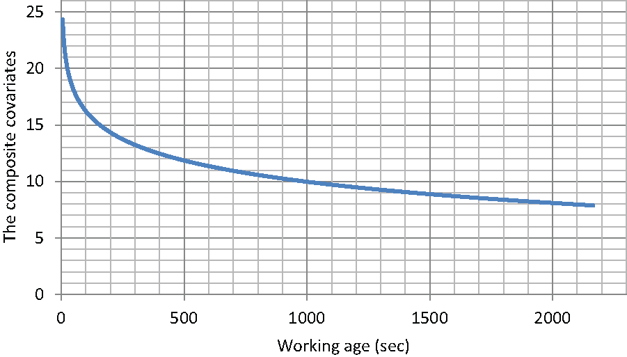
Optimal replacement function-availability analysis.
In practice, finding optimal replacement policy is generalized. Figure 7 shows the sequence of finding the optimal replacement
Extract the event (tool failure) by sequential inspections for any machining process.
Collect the experimental data in order to build the model by estimating the parameters of the PHM.
Check the goodness of fit using, for example, Kolmogorov–Smirnov test.
Find
Calculate
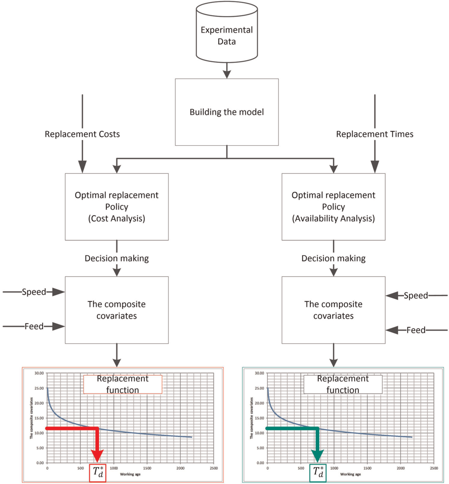
Finding the optimal replacement time in cost and availability analysis.
Practical use and sensitivity analysis
The replacement function is used for a single cutting tool in multitasked machining process under variable machining conditions. For example, the user may use the tool for machining a part with machining conditions
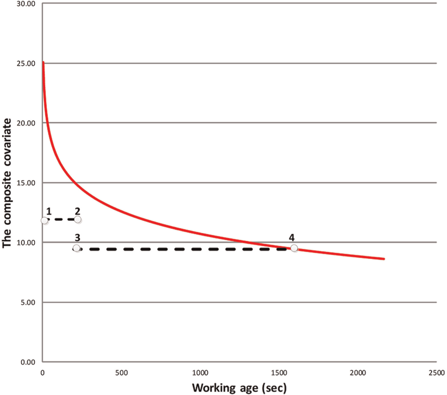
Optimal replacement example-cost analysis.
Sensitivity analysis is performed on the cost ratio (r). Figure 9 shows the cost ratio sensitivity when r = 2 to r = 5. Obviously, the optimal time to replacement is decreasing when the cost ratio (r) is increasing. This is very logical because as the difference between the failure replacement cost and the preventive replacement cost gets higher, the more frequent preventive replacement should be done, thus the new optimal time to replacement will be less than the original one, in order to minimize the cost per unit time.
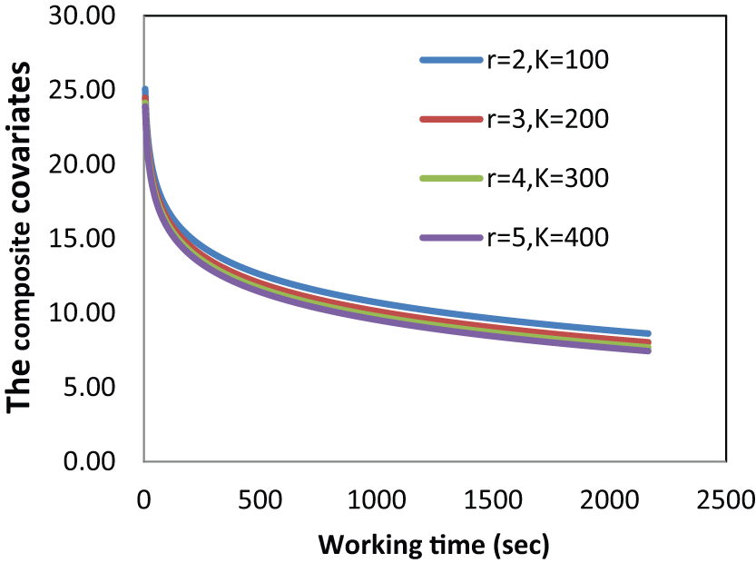
The cost ratio sensitivity.
Conclusion
In this article, we have introduced two new contributions to the research on tool replacement, which are two optimality models for cost minimization and availability maximization, and we applied it to a new generation of composites, namely, the TiMMCs. Experimentally, data were collected during turning TiMMCs under variable machining conditions. The collected data were used to construct the PHM. The PHM offered a statistically good model for the problem. An optimal replacement function was obtained and built into a simple chart. While changing the machining conditions, we showed how the user can find the optimal time to replacement that optimizes either the machining cost or the availability per unit time. In these cases, the machining cost per unit time and availability were found to be equal to 0.13 $/s and 80.77%, respectively. If these models are not used, the run to failure cost and availability are found to be 0.20 $/s and 64.57%, respectively. This represents a saving of 35.7% in case of cost analysis and an increasing of 16.20% in the case of availability analysis.
Footnotes
Appendix 1
Declaration of conflicting interests
The author(s) declared no potential conflicts of interest with respect to the research, authorship, and/or publication of this article.
Funding
The author(s) disclosed receipt of the following financial support for the research, authorship, and/or publication of this article: This research is funded by Natural Science and Engineering Research Council of Canada (NSERC), and Natural and Technology Research Fund of Quebec (FQRNT).