Sage Journals: Discover world-class research

Abstract

The objective of this study is to model the temperature distributions in milling analytically. In this article, previous research on heat generation and heat dissipation in the machining process was reviewed and then the temperature model in intermittent cutting with continuously varying chip thickness was established. The experimental study to measure cutting temperature in milling Ti6Al4V utilizing semi-artificial thermocouple was presented. The predicted and experimental results for milling process were presented and compared. The results showed that the proposed mathematical model could predict cutting temperature with high accuracy.

Keywords

Cutting parameter end milling semi-artificial thermocouple temperature Ti6Al4V

Introduction

Thermal effects and measurements of temperature distribution in the cutting tool and workpiece are of central interest in the context of tool performance and machinability of workpiece materials.^1–6 Taylor,⁷ Trigger and Chao⁸ and Hahn⁹ carried out the analytical evaluations of cutting temperature decades ago. Loewen and Shaw¹⁰ discussed the influence of variables on the cutting temperature. Usui et al.,¹¹ Tlusty and Orady¹² and Smith and Armarego¹³ used the finite difference method to predict the steady-state temperature distribution in continuous machining by utilizing the predicted quantities, such as chip formation and cutting forces, through the energy method. Komanduri and Hou^14–16 and Huang and Liang^17,18 discussed and established the steady-state temperature model in metal cutting based on the premise of a moving heat source, which was applied for high-speed machining by Abukhshim et al.¹⁹ In order to illustrate the relationship between the cutting temperature and the yield stress of the machined material, Vorontsov et al.^20,21 derived the specific formulas for thermal processes in cutting. Meanwhile, M’Saoubi and Chandrasekaran²² introduced the variable between frictional heat source and secondary shear based on the experimental study. Stephenson and Ali²³ conducted the model considering the interrupted cutting with constant chip thickness. The numerical model based on the finite difference method to predict tool and chip temperature fields in milling processes was presented by Lazoglu and Altintas.²⁴ Furthermore, List et al.,²⁵ Sato et al.,²⁶ Yashiro et al.²⁷ and Sun et al.²⁸ also researched the methods to measure temperature.

Unfortunately, there has been less research reported in the prediction of tool temperature in milling, where the chip thickness varies continuously, and the process is intermittent (i.e. the tool periodically enters and exits the cut). The objective of this study is to analytically model the temperature distributions in milling. First, the previous research on heat generation and distribution in the machining process was reviewed and then temperature model in milling with continuously varying chip thickness was established, as described in section “Mathematical model of cutting temperature.” Second, the experimental study to measure cutting temperature in milling Ti6Al4V utilizing semi-artificial thermocouple was carried out, and the predicted and experimental results for milling process were presented and compared, as described in section “Experimental analysis and model validation.”

Mathematical model of cutting temperature

In this section, the heat source was introduced simply and the basic assumptions were presented first. Then, the temperature model of tool, chip and workpiece in oblique cutting were reviewed, and cutting temperature model in milling with the continuously varying chip thickness was established.

Introduction and basic assumptions

There are two main heat sources in metal cutting, namely, primary heat source, as shown in Figure 1 ABCD, and secondary heat source, as shown in Figure 1 C′EFD′. On the chip side, the primary heat source was considered as a uniform moving oblique band heat source, and the secondary heat source was considered as a uniform moving band heat source within a semi-infinite medium. On the tool side, the effect of the secondary heat source was considered as uniform static rhomboid heat source in a semi-infinite medium along the tool–chip contact length.

Figure 1.

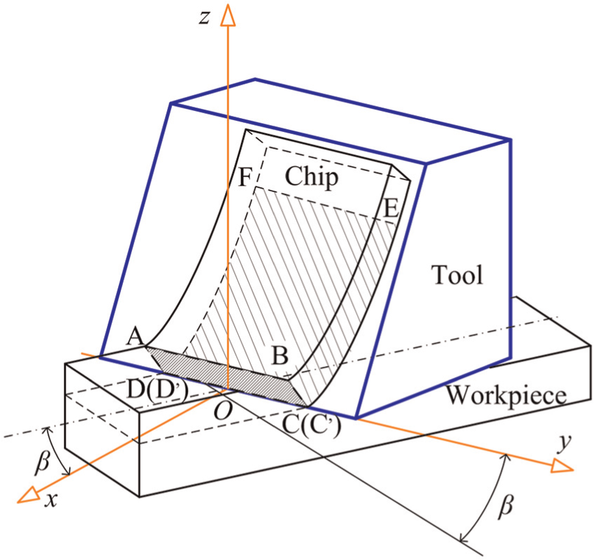
Heat sources.

The main assumptions employed in the development of temperature model are as follows:^17,18

The rubbing heat source between tool flank face and workpiece is negligible;

The generated heat flow and the temperature distribution are in steady state;

All of the deformation energy within the deformation zones is converted into heat;

The primary and the secondary heat sources are plane heat sources;

A cutting wedge angle of 90° is considered to simplify the problem, which is a good approximation for most of cutting tools;

The tool is “sharp” without any wear.

Modeling of chip side temperature

Modeling the effect of the primary heat source

The effect of the primary heat source on the chip side was modeled as an oblique moving band heat source moving within the chip under the surface BE of a semi-infinite body with a velocity v_ch as shown in Figure 2. The upper boundary of the semi-infinite body can be considered adiabatic. In order to convert the semi-infinite heat source into infinite heat source, an image heat source (a mirror image of the primary heat source with respect to the boundary surface) with the same heat flux density should be introduced. Therefore, the infinite heat source method is suitable for the semi-infinite heat source, as shown in Figure 2, and the chip side temperature field under the effect of the primary heat source can be given by equations (1)–(5)^14–18

T_{P} = T_{P_{1}} + T_{P_{2}}

(1)

\begin{matrix} T_{P_{1}} = \frac{q_{s} {dl}_{i}}{8 c ρ π a} \\ \int_{l_{i} = 0}^{l_{p}} \int_{0}^{t} \frac{e^{- \frac{P_{_{1}}^{2}}{4 a τ}}}{τ} [\erf (\frac{z}{\sqrt{4 a τ}}) - \erf (\frac{z - L_{p}}{\sqrt{4 a τ}})] d τ {dl}_{i} \end{matrix}

(2)

\begin{matrix} T_{P_{2}} = \frac{q_{s} {dl}_{i}}{8 c ρ π a} \\ \int_{l_{i} = 0}^{l_{p}} \int_{0}^{t} \frac{e^{- \frac{P_{_{2}}^{2}}{4 a τ}}}{τ} [\erf (\frac{z}{\sqrt{4 a τ}}) - \erf (\frac{z - L_{p}}{\sqrt{4 a τ}})] d τ {dl}_{i} \end{matrix}

(3)

P_{1} = \sqrt{{(x - l_{i} \sin ϕ + v_{ch} τ)}^{2} + {(l_{i} \cos ϕ - y)}^{2}}

(4)

P_{2} = \sqrt{{(x - l_{i} \sin ϕ + v_{ch} τ)}^{2} + {(l_{i} \cos ϕ + y)}^{2}}

(5)

Figure 2.

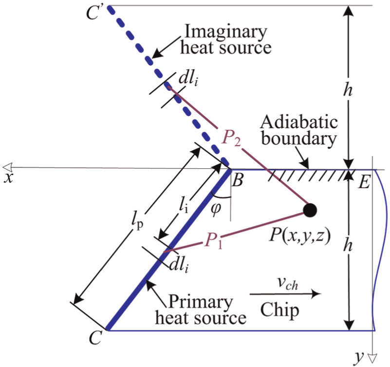
Heat transfer model of primary heat source.

Modeling the effect of the secondary heat source

As shown in Figure 3, by considering the secondary heat source as the obliquely moving band heat source with a velocity v_ch, the temperature rise on the chip side due to the secondary heat source can be expressed as^14–18

T_{D} = T_{D_{1}} + T_{D_{2}}

(6)

\begin{matrix} T_{D_{1}} = \frac{q_{f} {dl}_{i}}{8 c ρ π a} \\ \int_{l_{i} = 0}^{l_{s}} \int_{0}^{t} \frac{e^{- \frac{D_{1}^{2}}{4 a τ}}}{τ} [\erf (\frac{z}{\sqrt{4 a τ}}) - \erf (\frac{z - L_{s}}{\sqrt{4 a τ}})] d τ {dl}_{i} \end{matrix}

(7)

\begin{matrix} T_{D_{2}} = \frac{q_{f} {dl}_{i}}{8 c ρ π a} \\ \int_{l_{i} = 0}^{l_{s}} \int_{0}^{t} \frac{e^{- \frac{D_{2}^{2}}{4 a τ}}}{τ} [\erf (\frac{z}{\sqrt{4 a τ}}) - \erf (\frac{z - L_{s}}{\sqrt{4 a τ}})] d τ {dl}_{i} \end{matrix}

(8)

D_{1} = \sqrt{{(x - l_{i} + v_{ch} τ)}^{2} + y^{2}}

(9)

D_{2} = \sqrt{{(x - l_{i} + v_{ch} τ)}^{2} + {(2 h - y)}^{2}}

(10)

Figure 3.

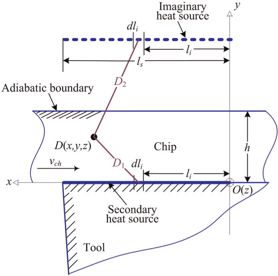
Heat transfer model of the secondary heat source relative to the chip side.

Modeling of tool side temperature along the tool–chip interface in oblique cutting

For a fresh tool, the chip may be considered as a rhomboid band uniform heat source sliding in oblique cutting with the velocity v_ch over a motionless semi-infinite body (the tool) which insulated the boundary condition along the tool flank face.^4,5 As shown in Figure 4, the temperature rise on the tool side due to the secondary heat source can be expressed as^14–18

T_{M} = \frac{q_{f}}{2 π λ_{t}} \int_{z_{i} = 0}^{L_{ts}} {dz}_{i} \int_{x_{i} = 0}^{l_{s}} (\frac{1}{M_{1}} + \frac{1}{M_{2}}) {dx}_{i}

(11)

M_{1} = \sqrt{{(x - x_{i})}^{2} + y^{2} + {(z_{i} \cos β - z)}^{2}}

(12)

M_{2} = \sqrt{{(x - 2 l_{s} + x_{i})}^{2} + y^{2} + {(z_{i} \cos β - z)}^{2}}

(13)

Figure 4.

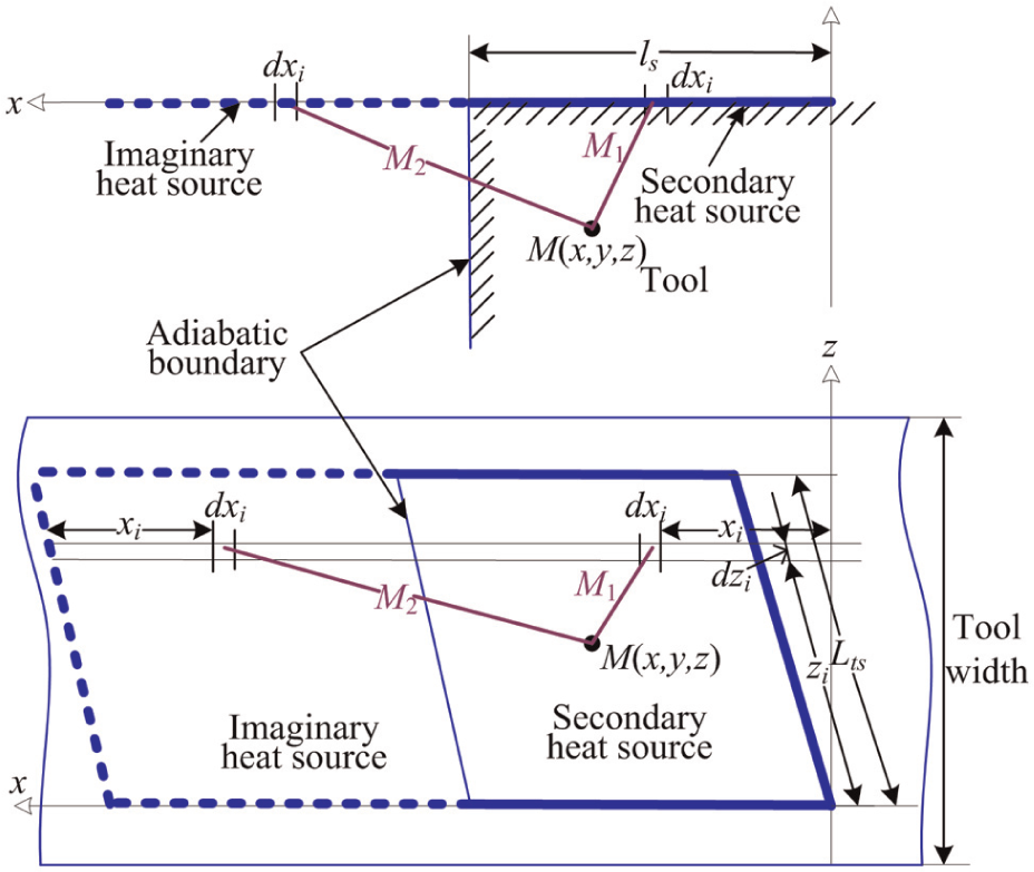
Heat transfer model of the secondary heat source relative to the tool side.

Temperature modeling under the comprehensive effect of the primary and secondary heat sources

Figure 5 shows a schematic representation of the heat transfer model of the two principal heat sources in metal cutting: the primary heat source CB and the secondary heat source CE operate simultaneously in the local coordinate system.

Figure 5.

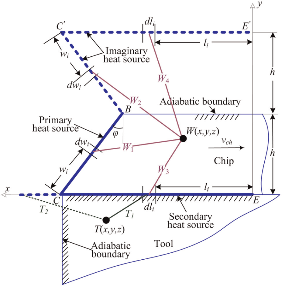
Temperature modeling under the comprehensive effect of the primary and secondary heat sources.

The total temperature rise at any point W(x, y, z) on the chip side could be shown to be

T_{W} = T_{W_{1}} + T_{W_{2}} + T_{W_{3}} + T_{W_{4}}

(14)

\begin{matrix} T_{W_{1}} = \frac{q_{s}}{8 c ρ π a} \\ \int_{w = 0}^{h / \cos (ϕ - α)} \int_{0}^{t} \frac{e^{- \frac{W_{1}^{2}}{4 a τ}}}{τ} [\erf (\frac{z}{\sqrt{4 a τ}}) - \erf (\frac{z - L_{ts}}{\sqrt{4 a τ}})] d τ {dw}_{i} \end{matrix}

(15)

\begin{matrix} T_{W_{2}} = \frac{q_{s}}{8 c ρ π a} \\ \int_{w = 0}^{h / \cos (ϕ - α)} \int_{0}^{t} \frac{e^{- \frac{W_{2}^{2}}{4 a τ}}}{τ} [\erf (\frac{z}{\sqrt{4 a τ}}) - \erf (\frac{z - L_{ts}}{\sqrt{4 a τ}})] d τ {dw}_{i} \end{matrix}

(16)

\begin{matrix} T_{W_{3}} = \frac{q_{f}}{8 c ρ π a} \\ \int_{l_{i} = 0}^{l_{s}} \int_{0}^{t} \frac{e^{- \frac{W_{3}^{2}}{4 a τ}}}{τ} [\erf (\frac{z}{\sqrt{4 a τ}}) - \erf (\frac{z - L_{ts}}{\sqrt{4 a τ}})] d τ {dl}_{i} \end{matrix}

(17)

\begin{matrix} T_{W_{4}} = \frac{q_{f}}{8 c ρ π a} \\ \int_{l_{i} = 0}^{l_{s}} \int_{0}^{t} \frac{e^{- \frac{W_{4}^{2}}{4 a τ}}}{τ} [\erf (\frac{z}{\sqrt{4 a τ}}) - \erf (\frac{z - L_{ts}}{\sqrt{4 a τ}})] d τ {dl}_{i} \end{matrix}

(18)

W_{1} = \sqrt{{(x - x_{i} + v τ)}^{2} + {(y - y_{i})}^{2}}

(19)

W_{2} = \sqrt{{(x - x_{i} + v τ)}^{2} + {(2 h - y - y_{i})}^{2}}

(20)

W_{3} = \sqrt{{(x - l_{i} + v τ)}^{2} + y^{2}}

(21)

W_{4} = \sqrt{{(x - l_{i} + v τ)}^{2} + {(2 h - y)}^{2}}

(22)

where x_i = l_s − w_isin(ϕ − α) and y_i = w_icos(ϕ − α).

The total temperature rise at any point T(x, y, z) on the tool side could be estimated by

\begin{matrix} T_{T} = \frac{q_{f}}{2 π λ_{t}} \int_{z_{i} = 0}^{L_{ts}} {dz}_{i} \int_{l_{i} = 0}^{l_{s}} (\frac{1}{T_{1}} + \frac{1}{T_{2}}) {dx}_{i} \\ + \frac{q_{fs}}{2 π λ_{t}} \int_{z_{i} = 0}^{L_{ts}} {dz}_{i} \int_{l_{i} = 0}^{l_{s}} (\frac{1}{T_{1}} + \frac{1}{T_{2}}) {dx}_{i} \end{matrix}

(23)

T_{1} = \sqrt{{(x - x_{i})}^{2} + y^{2} + {(z_{i} \cos β - z)}^{2}}

(24)

T_{2} = \sqrt{{(x - 2 l_{s} + x_{i})}^{2} + y^{2} + {(z_{i} \cos β - z)}^{2}}

(25)

It is assumed that the temperature rise on the chip side and on the tool side along the tool–chip interface should be equal as follows^17,18

T_{W} (x, 0, z) = T_{T} (x, 0, z)

(26)

Temperature modeling in milling process

In the previous sections, the mathematical analysis and modeling to determine the steady-state tool and chip temperatures were described. However, it is also important to know temperature generation and distribution for the high-speed milling process, in which the contact between tool and workpiece is intermitted, and the chip thickness varies continuously with the spindle rotation (i.e. with time). The temperature rises during the cutting process due to the generated shear and frictional heat and decreases during the noncutting period due to the air cooling. Figure 6 shows the adopted approach to predict cutting temperature for the end milling process.

Figure 6.

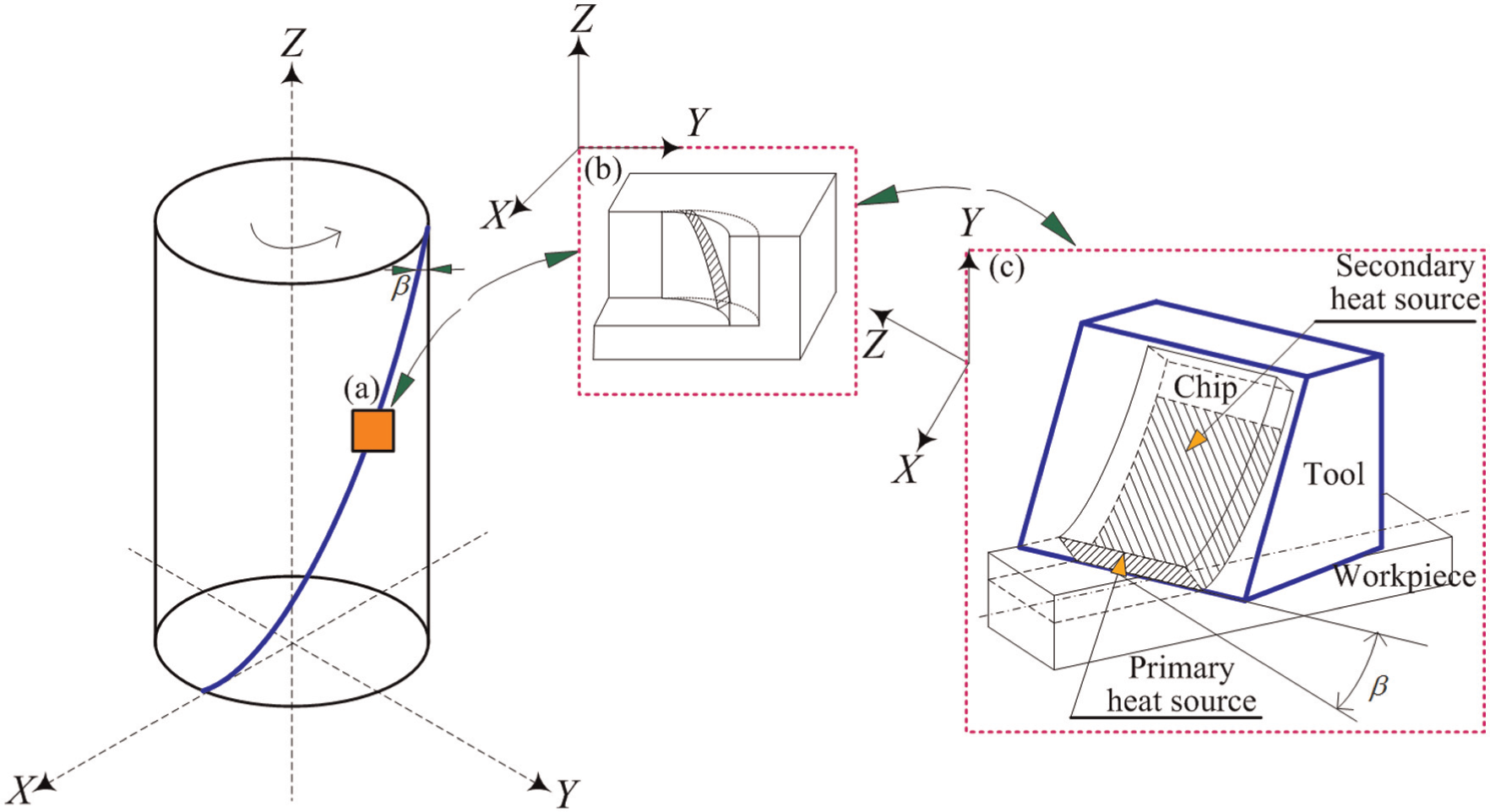
Adopted approach to predict cutting temperature for the end milling process: (a) tool element, (b) heat transfer model and (c) oblique cutting.

It is well known that the milling process is typically interrupted machining, and the tool enters and exits the workpiece periodically. Hence, the energy created in the primary and secondary zones varies with time. Moreover, the milling machining is also a typical oblique cutting process. Therefore, knowing the steady-state temperature fields in oblique cutting and giving the time constant of the milling process will be sufficient to predict the transient temperature. So, the steady-state temperature for the milling process can be determined for a given set of time inputs by utilizing the temperature model shown in the previous sections.

As shown in Figure 6, the power generated per unit depth of cut in the primary and secondary zones are, respectively, given as follows

Q_{s} = F_{s} \cdot v_{s}

(27)

F_{s} = \sqrt{[{(F_{a} \cos β - F_{t} \sin β)}^{2} + {(F_{a} \cos β \cos ϕ - F_{r} \sin ϕ + F_{t} \cos β \cos ϕ)}^{2}]}

(28)

v_{s} = \frac{v \cos β \cdot \sin ϕ}{\cos η_{s}} [\tan (ϕ - α) + \frac{1}{\tan ϕ}]

(29)

Q_{f} = F_{f} \cdot v_{ch}

(30)

F_{f} = \frac{F_{r} \cos α + F_{t} \sin α}{\cos η_{s}}

(31)

v_{ch} = \frac{v \cos β \sin ϕ}{\cos η_{s} \cos (ϕ - α)}

(32)

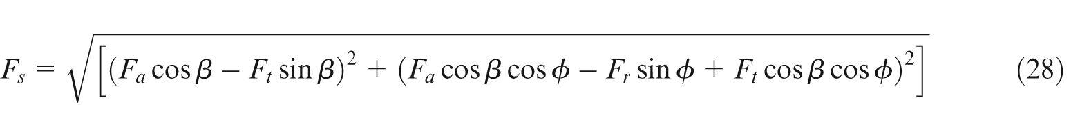
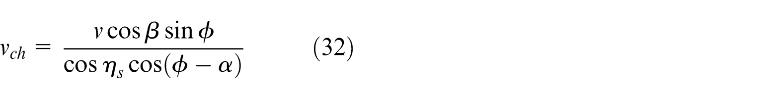
As described earlier, F_a is axial cutting force, F_t is tangential cutting force and F_r is radial cutting force. The mathematical equations for the cutting force prediction models under oblique cutting process can be given by equation (33) ^29–31

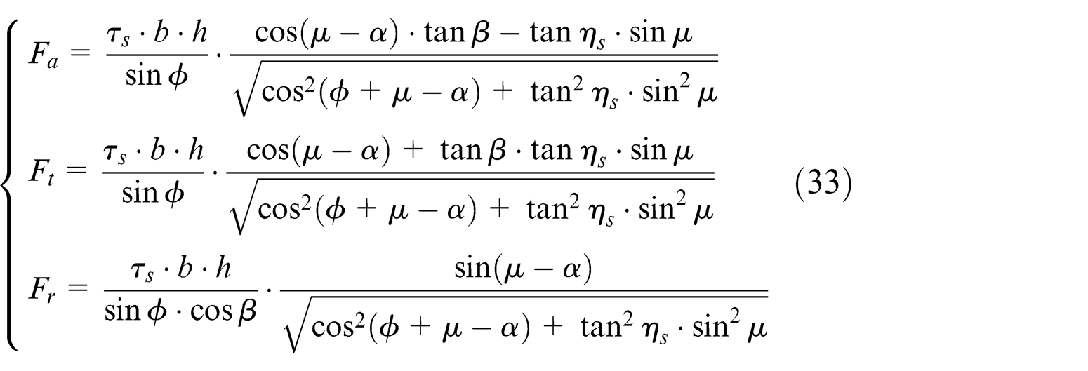
{\begin{matrix} F_{a} = \frac{τ_{s} \cdot b \cdot h}{\sin ϕ} \cdot \frac{\cos (μ - α) \cdot \tan β - \tan η_{s} \cdot \sin μ}{\sqrt{\cos^{2} (ϕ + μ - α) + \tan^{2} η_{s} \cdot \sin^{2} μ}} \\ F_{t} = \frac{τ_{s} \cdot b \cdot h}{\sin ϕ} \cdot \frac{\cos (μ - α) + \tan β \cdot \tan η_{s} \cdot \sin μ}{\sqrt{\cos^{2} (ϕ + μ - α) + \tan^{2} η_{s} \cdot \sin^{2} μ}} \\ F_{r} = \frac{τ_{s} \cdot b \cdot h}{\sin ϕ \cdot \cos β} \cdot \frac{\sin (μ - α)}{\sqrt{\cos^{2} (ϕ + μ - α) + \tan^{2} η_{s} \cdot \sin^{2} μ}} \end{matrix}

(33)

where b is the width of cutting; h is the cutting layer thickness (h = f_z·sin ψ for end milling, where f_z is the feed rate and ψ represents the angular position of the cutting point); η_s is the chip flow angle; and β = η_s based on Stabler’s chip flow law.³²

The heat flux density between primary heat source q_s and secondary heat source q_f is described as follows

q_{s} = \frac{Q_{s}}{A_{s}} = \frac{F_{s} \cdot v_{s}}{(b / \cos β) \cdot f_{z} \cdot \sin ψ}

(34)

\begin{matrix} q_{f} & = \frac{Q_{f}}{A_{f}} = \frac{F_{f} \cdot v_{c}}{(b / \cos β) \cdot l_{c}} \\ = \frac{F_{f} \cdot v_{c}}{(b / \cos β) f_{z} \sin ψ [\sin (ϕ - α) + (\cos η_{s}) \tan μ \cos (ϕ - α)]} \end{matrix}

(35)

The temperature model in section “Temperature modeling under the comprehensive effect of the primary and secondary heat sources” is in the local coordinate system (x, y, z) as shown in Figure 7. Therefore, the cutting temperature in the overall coordinate system (X, Y, Z) could be transformed from the local coordinate according to the following equation (36)

[\begin{matrix} x \\ y \\ z \\ 1 \end{matrix}] = [\begin{matrix} \cos ψ & \sin ψ & 0 & - R \\ \sin ψ & - \cos ψ & 0 & 0 \\ 0 & 0 & 1 & 0 \\ 0 & 0 & 0 & 1 \end{matrix}] [\begin{matrix} X \\ Y \\ Z \\ 1 \end{matrix}]

(36)

Figure 7.

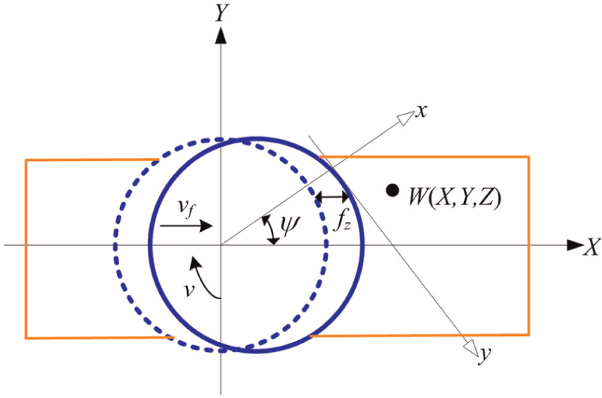
Milling coordinate diagram.

So, when $ψ$ is variable from ψ_en to ψ_ex, the heat generated in milling process is given as equation (37)

T = \int_{ψ_{en}}^{ψ_{ex}} T_{W} (x, 0, z) d ψ + T_{0} = \int_{ψ_{en}}^{ψ_{ex}} T_{T} (x, 0, z) d ψ + T_{0}

(37)

where T₀ is the room temperature.

Experimental analysis and model validation

In order to verify the validity and capability of the temperature model, the end milling Ti6Al4V experiment with solid carbide tool was set up, and the temperature was measured by semi-artificial thermocouple in the machining process. In this section, temperature measurement principle was introduced briefly and then the experimental set-up and cutting parameters were presented. Finally, the comparison between measured results and predicted results was carried out and discussed.

Experimental principle

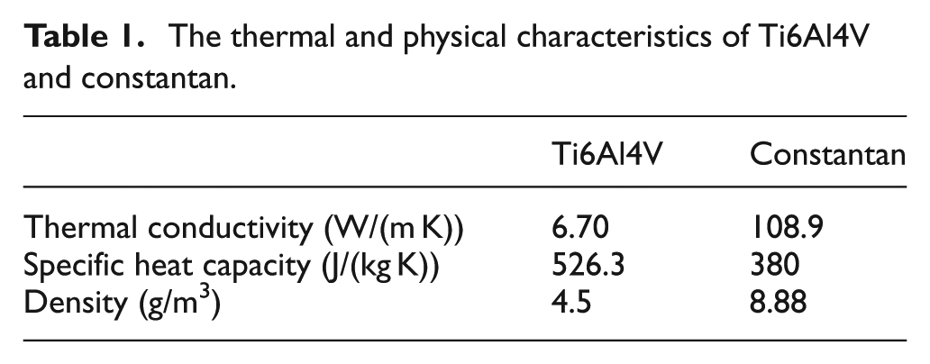
The semi-artificial thermocouple was utilized to obtain the cutting temperature, which was composed of Ti6Al4V and constantan with excellent electrical conductivity, as shown in Figure 8. In order to obtain temperature values of milling process for more time, the constantan belt was applied in this study. The thermal and physical characteristics of Ti6Al4V and constantan used in calculations are shown in Table 1.

Table 1.

The thermal and physical characteristics of Ti6Al4V and constantan.

	Ti6Al4V	Constantan
Thermal conductivity (W/(m K))	6.70	108.9
Specific heat capacity (J/(kg K))	526.3	380
Density (g/m³)	4.5	8.88

Figure 8.

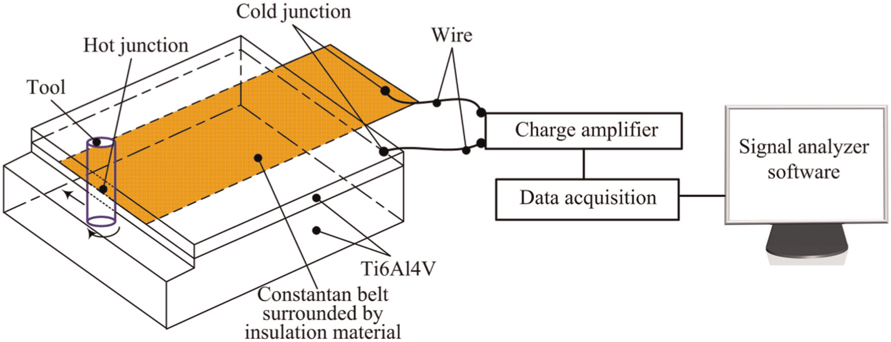
Schematic representation of semi-artificial thermocouple temperature measurement device.

As shown in Figure 8, the thin constantan belt surrounded by insulation material was embedded into Ti6Al4V specimen, which was split into two parts and polished in advance. In this way, the semi-artificial thermocouple can be in contact with the machining area directly. In the cutting process, insulation material was cut open, and the hot junctions were created between constantan belt and Ti6Al4V specimen to measure local temperature. The cold junctions were on constantan belt and Ti6Al4V specimen far away from processing area, respectively, where temperature had little change. The thermal electromotive force was produced between the cold junctions due to the temperature imposed on the hot junctions based on the Seebeck effect, reported as the thermal electromotive force generated by the temperature gradient detected at different metal contacts. The output voltage signals were first amplified by a high-resolution and high-frequency charge amplifier and then transmitted to the data acquisition device. Finally, the temperature during the machining could be recorded through the data acquisition or analysis software in computer.

Calibration of Ti6Al4V-constantan thermocouple

Since the Ti6Al4V-constantan is not a standard thermocouple, there is no relational data between temperature and thermal electromotive force of this thermocouple. Therefore, it has the necessity for an accurate calibration of the Ti6Al4V and constantan materials as a thermocouple pair to get the corresponding relationship between thermal electromotive force and temperature, which will provide reliable basis for experimental data processing.

The calibration was conducted in the resistance furnace, as shown in Figure 9. Figure 10 shows the thermocouple calibration curve for Ti6Al4V-constantan thermocouple.

Figure 9.

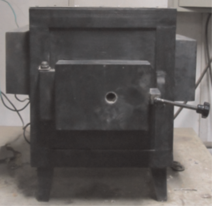
Resistance furnace.

Figure 10.

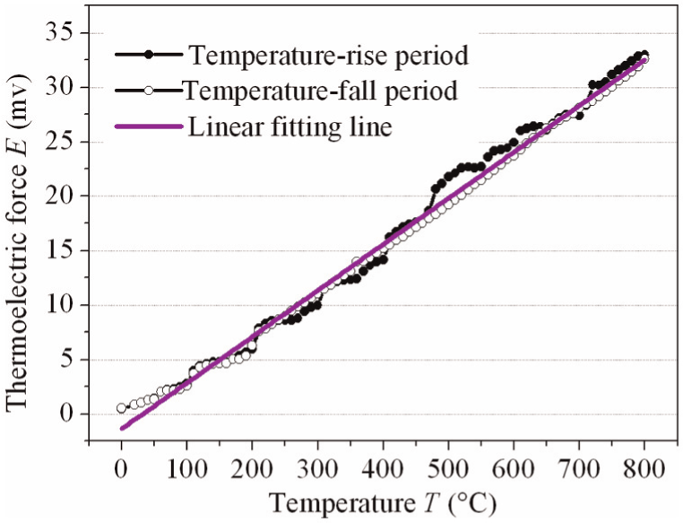
Thermocouple calibration curve.

The relationship between thermal electromotive force and temperature could be approximated using the linear fitting, represented by equation (38)

E = 0.042 T - 1.3742

(38)

where E is the thermoelectric potential and T is the temperature.

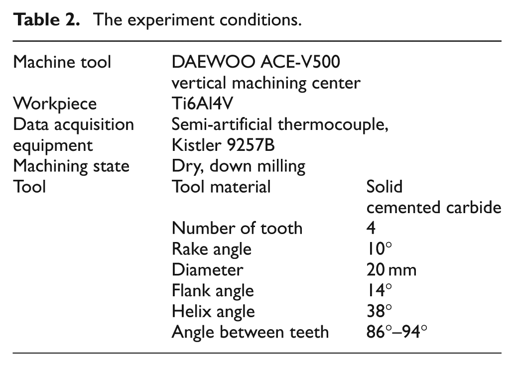
Experimental conditions and cutting parameters

The experimental conditions are shown in Table 2.

Table 2.

The experiment conditions.

Machine tool	DAEWOO ACE-V500 vertical machining center
Workpiece	Ti6Al4V
Data acquisition equipment	Semi-artificial thermocouple, Kistler 9257B
Machining state	Dry, down milling
Tool	Tool material	Solid cemented carbide
	Number of tooth	4
	Rake angle	10°
	Diameter	20 mm
	Flank angle	14°
	Helix angle	38°
	Angle between teeth	86°–94°

In order to guarantee the stability and effectiveness of the thermoelectric potential signals, it should be insulated among Ti6Al4V, constantan belt, clamp and machine tool. Some insulating materials were utilized in the experiments, including insulating board and insulating paper, as shown in Figure 11.

Figure 11.

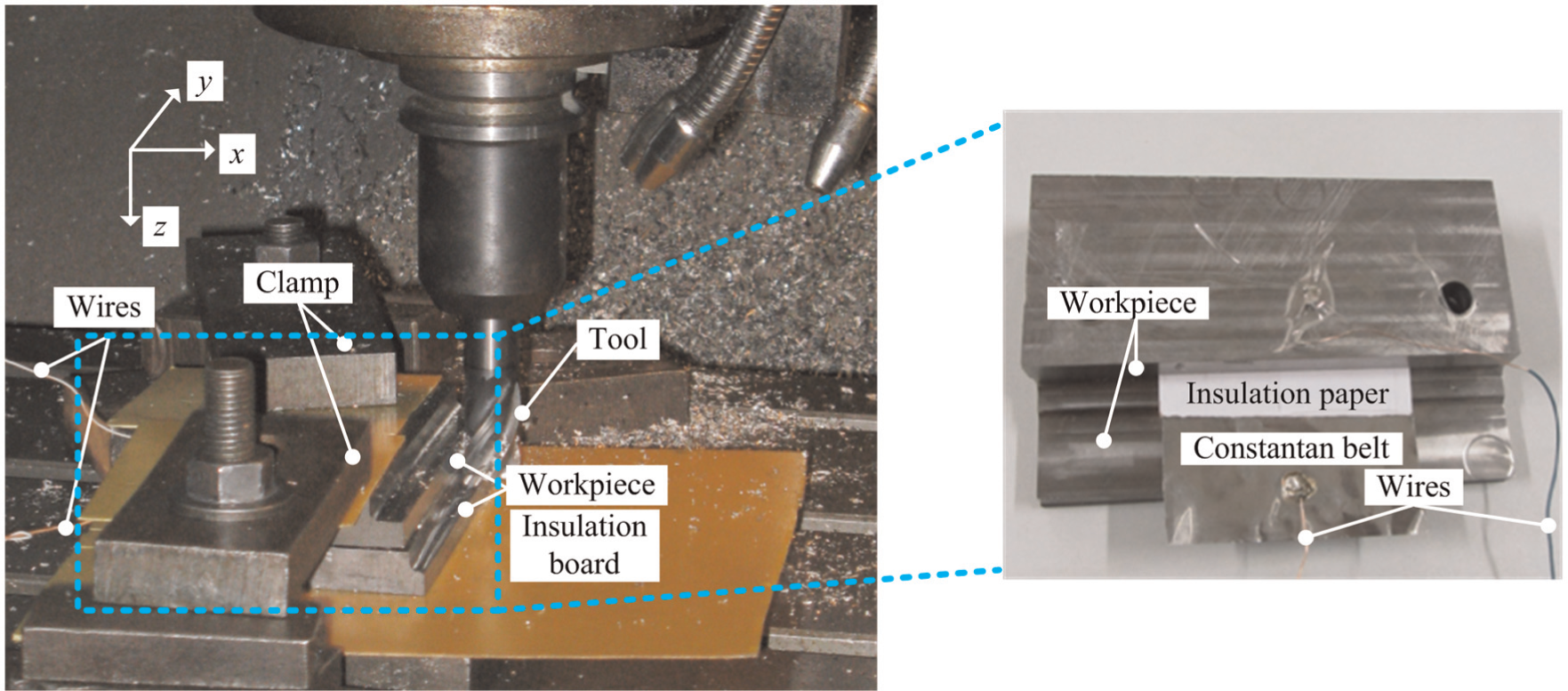
Experimental set-up.

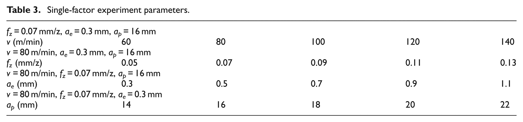
Cutting temperature is one of the significant physical variables in machining process and influenced by cutting speed, feed rate, radial feed and axial feed. The single-factor experiment was conducted, which could validate the model of temperature and is an effective method of intuitive expression of the influence of cutting parameters on the temperature. Table 3 lists the cutting parameters used in single-factor experiment.

Table 3.

Single-factor experiment parameters.

f_z = 0.07 mm/z, a_e = 0.3 mm, a_p = 16 mm
v (m/min)	60	80	100	120	140
v = 80 m/min, a_e = 0.3 mm, a_p = 16 mm
f_z (mm/z)	0.05	0.07	0.09	0.11	0.13
v = 80 m/min, f_z = 0.07 mm/z, a_p = 16 mm
a_e (mm)	0.3	0.5	0.7	0.9	1.1
v = 80 m/min, f_z = 0.07 mm/z, a_e = 0.3 mm
a_p (mm)	14	16	18	20	22

Comparison between measured results and predicted results

The comparisons of maximum temperature along the tool–chip interface between measured results and predicted results for the above conditions were discussed, and the quantitative comparisons between them were carried out to examine the adequacy of the models, as shown in Figure 12. The comparisons were based on the percentage deviations of the predicted values with respect to the corresponding measured data using the following equation

% deviations = \frac{T_{Measured} - T_{Predicted}}{T_{Measured}} \times 100

(39)

Figure 12.

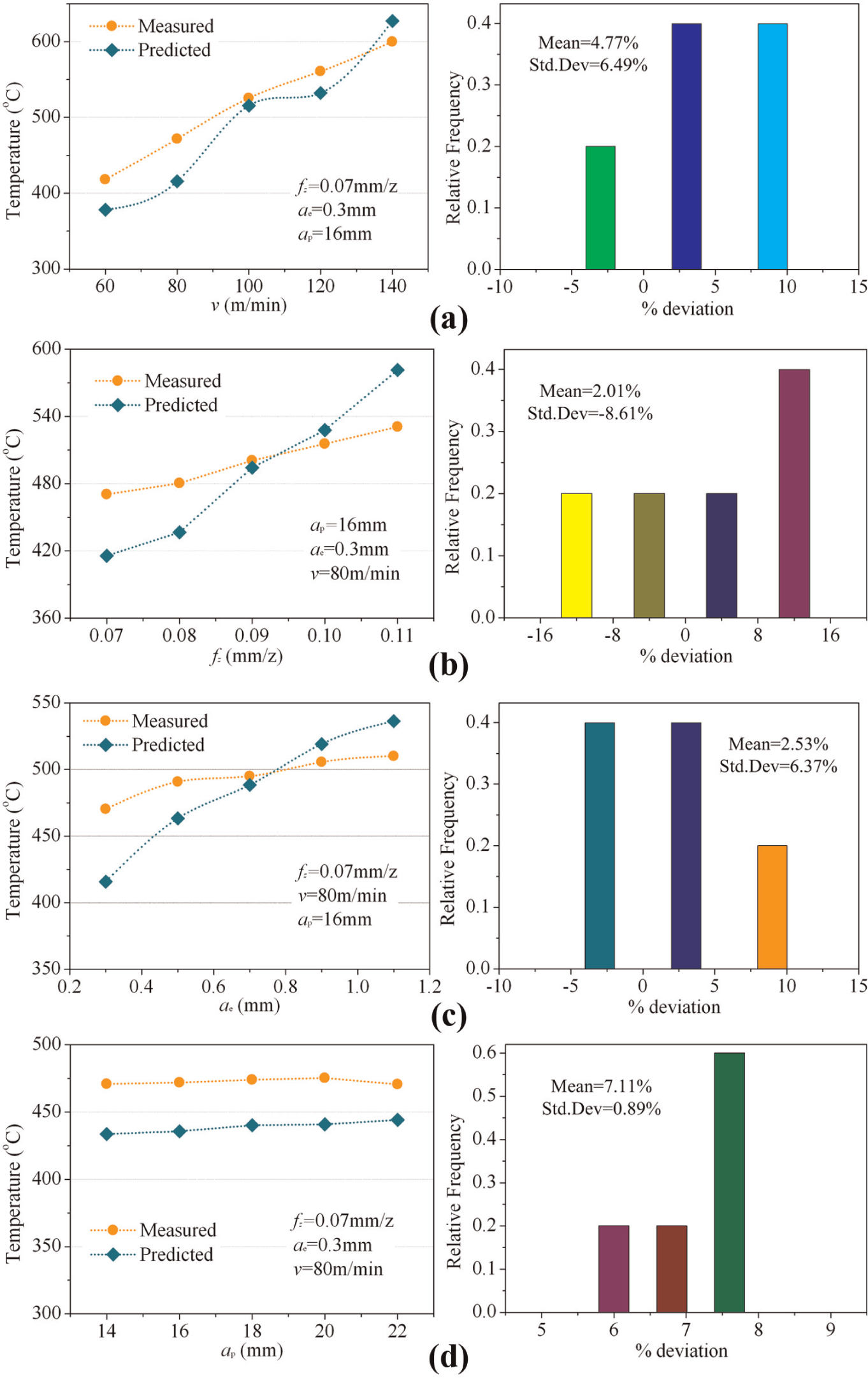
The maximum temperature at the tool–chip interface as a function of (a) cutting speed v and the histograms for percentage deviation, (b) feed rate f_z and the histograms for percentage deviation, (c) radial feed a_e and the histograms for percentage deviation and (d) axial feed a_p and the histograms for percentage deviation.

where T_Measured is the measured temperature and T_Predicted is the predicted temperature.

The variation of cutting temperature with cutting speed is shown in Figure 12(a). Obviously, it is seen that temperature ascends with the increase in cutting speed. Generally, a considerable amount of the machine energy is converted into heat through more critical plastic deformation of the workpiece and more friction between the chip and the tool rake face with the increase in cutting speed, which generates the increment in temperature.

The influence of feed rate on measured temperature is shown in Figure 12(b). It is found that cutting temperature increases with the increase in feed rate in milling process, and the variation of temperature has a similar trend following Figure 12(a). However, the tendency of increase is milder than that of cutting speed. It is because the thicker chip which carries off more thermal is produced with the increase in feed rate.

It can be found that the influence of radial feed on temperature is similar to that of cutting speed and feed rate on temperature, as shown in Figure 12(c), and the tendency of increase is even milder on account of there being benign heat dissipation area for greater radial feed.

As shown in Figure 12(a)–(c), temperature presents a similar rise trend with the increase in cutting speed, feed rate and radial feed. Figure 12(d) shows that the temperature is almost invariant with the increase in axial feed, which suggests that the axial feed has the least effect on cutting temperature.

Figure 12(a)–(d) shows that the predicted results present a reasonably good agreement with the measured results. The histograms for overall comparison for both of the predicted and measured temperatures are also given in Figure 12. It is apparent that the average deviation in the maximum temperature is noticeable in the range of 2.01%−7.11%. It also shows that the model prediction gives a standard deviation in the range of −8.61% to 6.49%. These findings imply that the proposed model can give adequate prediction for the cutting temperature in end milling.

Meanwhile, it could be found that the predicted temperature is less than the measured temperature. Several possible reasons may explain the discrepancies. First, the contribution of rubbing heat source between the workpiece and the tool is ignored in this study. Second, the tool is “sharp” without any wear in this study, while it is necessary that tool wear being in end milling, which could also contribute to the increase in cutting temperature. Furthermore, in this study, the main assumptions were employed in the development of temperature model, such as all of the deformation energy within the deformation zones is converted into heat. Therefore, the quantity of heat disregarded in this case is negligible, which is one of factors that these generate the predicted temperature less than the measured temperature.

Based on the above-predicted model, the transient temperature at every time interval, which corresponds to a discrete cutter rotation angle for discretized chip thickness, is also obtained, and the comparison between measured results and predicted results is discussed, such as Figure 13, which shows the measured and predicted results for v = 80 m/min, f_z = 0.07 mm/z, a_e = 0.3 mm, a_p = 16 mm, cutter rotation angle from 1° to 14° and the histograms for percentage deviation between them.

Figure 13.

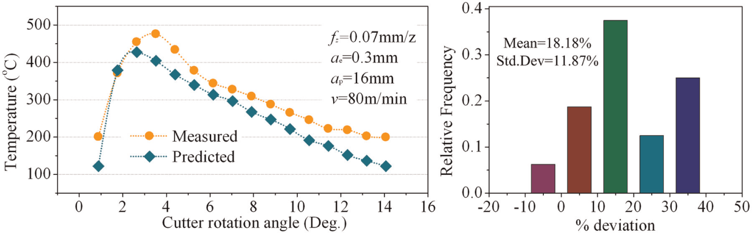
Transient tool–chip interface temperature prediction of the chip thickness discretization for end milling and the histograms for percentage deviation.

It can be seen that the predicted result agrees with that of the experiment. The histograms for comparison between them are also shown in Figure 13. It is apparent that the average deviation in the temperature is 18.18%. It also shows that the model prediction gives an 11.87% standard deviation. In conclusion, the comparison suggests reasonable accuracy of the predicted model. It could also be found that the predicted temperature is less than the measured one, and the reasons are mentioned above. It is worth noting that the appearance time of the maximum value in experiment is a little delaying than that of mathematical model for the retardation phenomenon of data collection system.

Conclusion

In this study, the temperature model for intermittent cutting with continuously varying chip thickness has been proposed. The end milling Ti6Al4V with solid carbide tool experiment was performed, and the cutting temperature was measured applying the semi-artificial thermocouple. The estimation of cutting temperature based on the developed model was compared to the experimental data. The major results obtained are as follows:

The experimental results presented that the temperature in end milling Ti6Al4V had the rising trend with the increase in cutting speed, feed rate and radial feed. The axial feed has the least effect on cutting temperature. The same conclusion could be drawn from mathematical prediction analysis.

An analysis of accuracy of the model was conducted by percentage deviations. The results showed that there was reasonable agreement between prediction and experiment.

Footnotes

Appendix 1 Declaration of conflicting interests

The authors declare that there is no conflict of interest.

Funding

This research was based on work supported by National Science & Technology Major Projects (grant no. 2012ZX04003021).

References

Jayakumar

Mathew

Joseph

. An investigation of cutting force and tool-work interface temperature in milling of Al-SiCp metal matrix composite. Proc IMechE, Part B: J Engineering Manufacture 2013; 227(3): 362–374.

Liu

Cai

Chen

. Investigation of cutting force and temperature of end-milling Ti–6Al–4V with different minimum quantity lubrication (MQL) parameters. Proc IMechE, Part B: J Engineering Manufacture 2011; 225(8): 1273–1279.

Palanisamy

Rajendran

Shanmugasundaram

. Prediction of cutting force and temperature rise in the end-milling operation. Proc IMechE, Part B: J Engineering Manufacture 2006; 220(10): 1577–1587.

O’Sullivan

Cotterell

. Workpiece temperature measurement in machining. Proc IMechE, Part B: J Engineering Manufacture 2002; 216(1): 135–139.

Jiang

Yan

. Optimizing end-milling parameters for surface roughness under different cooling/lubrication conditions. Int J Adv Manuf Tech 2011; 51: 841–851.

Jiang

Yan

Rong

. Radial turning of hardened AISI D2 steel with TiAlN coated inserts: simulations and experiments. Int J Adv Manuf Tech 2013; 64: 1555–1563.

Taylor

. On the art of cutting metals. Trans ASME 1907; 29: 231–248.

Trigger

Chao

. An analytical evaluation of metal cutting temperatures. Trans ASME 1951; 73: 57–68.

Hahn

. On the temperature developed at the shear plane in the metal cutting process. In: Proceedings of first U.S. National Congress of Applied Mechanics, Illinois Institute of Technology, Chicago, IL, 11–16 June 1951, pp.661–666.

10.

Loewen

Shaw

. On the analysis of cutting-tool temperatures. Trans ASME 1951; 76: 217–231.

11.

Usui

Shirakashi

Kitagawa

. Analytical prediction of three dimensional cutting process. Part 3: cutting temperature and crater wear of carbide tool. Trans ASME 1978; 100: 236–243.

12.

Tlusty

Orady

. Effect of thermal cycling on tool wear in milling. In: 9th NAMRC conference, Pennsylvania State University, University Park, PA, 19–22 May 1981.

13.

Smith

AJR

Armarego

EJA

. Temperature prediction in orthogonal cutting with a finite difference approach. CIRP Ann: Manuf Techn 1981; 30: 9–13.

14.

Komanduri

Hou

. Thermal modeling of the metal cutting process. Part 1: temperature rise distribution due to shear plane heat source. Int J Mech Sci 2000; 42: 1715–1752.

15.

Komanduri

Hou

. Thermal modeling of the metal cutting process. Part 2: temperature rise distribution due to frictional heat source at the tool-chip interface. Int J Mech Sci 2001; 43: 57–88.

16.

Komanduri

Hou

. Thermal modeling of the metal cutting process. Part 3: temperature rise distribution due to the combined effects of shear plane heat source and the tool-chip interface frictional heat source. Int J Mech Sci 2001; 43: 89–107.

17.

Huang

Liang

. Modeling of the cutting temperature distribution under the tool flank wear effect. Proc IMechE, Part C: J Mechanical Engineering Science 2003; 217: 1195–1208.

18.

Huang

Liang

. Cutting temperature modeling based on non-uniform heat intensity and partition ratio. Mach Sci Technol 2005; 9: 301–323.

19.

Abukhshim

Mativenga

Sheikh

. Heat generation and temperature prediction in metal cutting: a review and implications for high speed machining. Int J Mach Tool Manu 2006; 46: 782–800.

20.

Vorontsov

Sultan-Zade

Albagachiev

. Development of a new theory of thermal cutting processes 19. Determining the temperature fields and contact temperatures in cutting (Part 2). Russ Eng Res 2011; 31: 671–678.

21.

Vorontsov

Sultan-Zade

Albagachiev

. Development of a new theory of thermal cutting processes 17. Determining the temperature fields and contact temperatures in cutting (Part 3). Russ Eng Res 2011; 31: 471–478.

22.

M’Saoubi

Chandrasekaran

. Experimental study and modeling of tool temperature distribution in orthogonal cutting of AISI 316L and AISI 3115 steels. Int J Adv Manuf Tech 2011; 56: 865–877.

23.

Stephenson

Ali

. Tool temperatures in interrupted metal cutting. Trans ASME 1992; 114: 127–136.

24.

Lazoglu

Altintas

. Prediction of tool and chip temperature in continuous and interrupted machining. Int J Mach Tool Manu 2002; 42: 1011–1022.

25.

List

Sutter

Bouthiche

. Cutting temperature prediction in high speed machining by numerical modeling of chip formation and its dependence with crater wear. Int J Mach Tool Manu 2012; 54–55: 1–9.

26.

Sato

Aoki

Tanaka

. Variation of temperature at the bottom surface of a hole during drilling and its effect on tool wear. Int J Mach Tool Manu 2013; 68: 40–47.

27.

Yashiro

Ogawa

Sasahara

. Temperature measurement of cutting tool and machined surface layer in milling of CFRP. Int J Mach Tool Manu 2013; 70: 63–69.

28.

Sun

. An experimental investigation of the influence of cutting parameters on cutting temperature in milling Ti6Al4V by applying semi-artificial thermocouple. Int J Adv Manuf Tech 2014; 70(5–8): 765–773.

29.

McFeron

Chao

. Transient interface temperatures in plain peripheral milling. Trans ASME 1958; 80: 321–329.

30.

Altintas

. Manufacturing automation: metal cutting mechanics, machine tool vibrations, and CNC design. Cambridge: Cambridge University Press, 2000.

31.

Budak

Altinta

Armarego

EJA

. Prediction of milling force coefficients from orthogonal cutting data. Trans ASME 1996; 118: 216–224.

32.

Stabler

. The chip flow law and its consequences. Proceeding of the Fifth International Machine Tool Design and Research Conference, Oxford, UK: Pergamon Press, 1964, pp. 216–224.

Modeling and experimental study of temperature distributions in end milling Ti6Al4V with solid carbide tool

Abstract

Keywords

Introduction

Mathematical model of cutting temperature

Introduction and basic assumptions

Modeling of chip side temperature

Modeling the effect of the primary heat source

Modeling the effect of the secondary heat source

Modeling of tool side temperature along the tool–chip interface in oblique cutting

Temperature modeling under the comprehensive effect of the primary and secondary heat sources

Temperature modeling in milling process

Experimental analysis and model validation

Experimental principle

Calibration of Ti6Al4V-constantan thermocouple

Experimental conditions and cutting parameters

Comparison between measured results and predicted results

Conclusion

Footnotes

Appendix 1

Declaration of conflicting interests

Funding

References