A bi-level programming model for supply chain network optimization with assembly line balancing and push–pull strategy

Abstract

This article investigates how to simultaneously optimize both strategic and tactical decisions in the supply chain network design. For this purpose, a bi-level programming model is developed in which supply chain network design problem is considered as a strategic decision in the upper-level model, while the lower-level model contains the assembly line balancing as a tactical decision. In addition, the problem is extended to include push–pull strategy where decisions such as production amount and inventory level of each component in manufacturers are made. Based on the special structure of the model, a heuristic method is proposed to solve the developed bi-level model. A numerical example is employed to show the performance of proposed method in terms of feasibility and convergence. Finally, computational experiments on several problem instances are presented to demonstrate the applications of developed model and the solution method.

Introduction

In today’s competitive market, the design and management of supply chain network (SCN) is one of the most important and difficult issues managers encounter. Supply chain management (SCM) is one of the areas that has attracted much attention over the past few decades. The main objective in SCM is to integrate variety of entities, including suppliers, manufacturers, distribution centers, and customers to produce merchandises and to distribute them to some locations in an efficient way. These entities constitute a network that has to be designed appropriately. ¹

In SCM, multi levels of decisions need to be made on the time horizon with multiple objective functions. Decision levels can be categorized as long-term decisions (strategic level), mid-term decisions (tactical level) and short-term decisions (operational level). ² The strategic level generally corresponds to the optimization of network resources such as designing networks, location and determination of the number and capacity of facilities. ³ Therefore, supply chain network design (SCND) is one of the most important strategic decisions in SCM that sometimes called as strategic supply chain planning. ⁴ On the other hand, tactical decisions deal with production levels at all plants, assembly policy, inventory levels and lot sizes. Finally, in the operational level, all material flows are scheduled based on the decisions made in the two other levels. So, operational decisions mainly include short-term decisions, such as production planning and scheduling. ⁵ Since opening or closing a facility is a time-consuming and expensive process, changing network design is almost impossible in the short run. However, since tactical and operational decisions are dependent on strategic decisions, the configuration of SCNs will become a constraint for tactical and operational decisions. ⁶

To create an agile SCN, compatible and capable assembly line processes and logistics processes need to work simultaneously. For this purpose, supply chain functions should be incorporated in a comprehensive framework.^7,8 This incorporation should basically be made between two main processes of supply chain: SCND and assembly line balancing (ALB). Many automobile companies face this situation, where appropriate decisions lead to more reliability, accuracy and customer satisfaction. On the need for integrating SCND problem with ALB, it should be noted that the production operations are decisive factors for the optimization of SCN. ALB operations, which are one of the decisive factors, are the most common situations in SCNs caused due to the large number of components. At this point, two main aspects achieve vital importance in a supply chain. First, companies attempt to add maximum value by minimizing their own transportation costs at each stage of the supply chain. Second, companies try to optimize the operations of whole areas of the supply chain such as line balancing and the fixed costs of opened workstations. Thus, there is a close linkage between assembly line processes and logistics processes that necessitates the incorporation of them in SCN. Consequently, obtaining the optimal assembly line has a significant effect on the performance of the SCN.

The defined network in this article, including manufacturers, assemblers and customers, is designed based on push–pull strategy. In this strategy, the initial stages of the supply chain are operated based on push system, and the final stages are operated on pull strategy. The interface between the push-based stages and the pull-based stages is referred as the push–pull boundary. In a push–pull strategy, the push part is applied to the stage of the supply chain where long-term forecasts have small uncertainty and variability. On the other hand, the pull part is applied to the stage of the supply chain where uncertainty and variability are high, and thus, decisions are made only in response to real demand. In a push–pull based supply chain, inventory is minimized as it is designed to eliminate the safety stock by make-to-order and long cycle time is reduced by pre-arranging/pre-manufacturing portion of the supply.

One of the main contributions of this article is to model and solve a SCND problem with ALB using bi-level programming. According to the best of authors’ knowledge, there is no article in the related literature to address this issue. Bi-level programming (BLP) is a tool for modeling decentralized decisions which contains the objective(s) of the leader at its first level and that is of the follower at the second level. ⁹ When SCND and ALB decisions are made by two different decision-makers with interactions on each other, bi-level programming would be an appropriate modeling approach.

The most similar study to our work belongs to Paksoy et al. ⁷ The main objective of their article is to present the problem of integrating SCND and ALB problems. They developed a mixed-integer nonlinear programming (MINLP) formulation to model and solve the problem. However, they did not consider the bi-level nature of the problem. In addition, developing the push–pull strategy and making decisions such as production amounts and inventory levels of each component in manufacturers are the other contributions of this article.

The rest of this article has the following structure. Section Literature review” reviews the literature of SCND and ALB problems. Section “Problem description and formulation” provides the assumptions and mathematical formulation of the problem. Section “Solution method” introduces a heuristic method to solve the developed BLP model. In addition, a numerical example is given in section “Solution method” to show the application of the model and the proposed solution method. The computational experiments over several problem instances are conducted in section “Computational experiments.” Finally, section “Conclusion and future studies” is devoted to conclusions and some directions for future research.

Literature review

This section reviews related previous studies in the context of two research areas; one is SCND problem and the other is ALB problem.

SCND

A supply chain is considered as an integrated process in which a group of several organizations, such as suppliers, manufacturers, distributors and customers, work together to acquire raw materials with a view to convert them into end-products and then distribute to the customers. ¹ The management of this chain is a significant issue that has attracted the research attention over the past several decades. Many mathematical models have been developed for designing and optimizing the SCNs up to now. These models range from simple uncapacitated single-product facility location models ¹⁰ to complex capacitated multi-commodity models ¹¹ with the aim of cost minimization or profit maximization. Most of the models in SCM field focus on the distribution/transportation networks with various considerations such as facility location, network design, demand satisfaction, warehousing and so on. ⁷

Recently, there has been a growing emphasis on practical aspects of SCNs, driving industrial practitioners to develop a comprehensive framework for supply chains. Srai et al. ¹³ propose a process maturity model-based alternative to SCN carbon measurement approaches, and present application of the maturity model framework in 12 case studies of international manufacturing multinationals to demonstrate feasibility and utility of the approach for industrial SCN. Xu et al. ¹⁴ develop a comprehensive framework of supply chain for product-service system based on the findings of a half-year investigation in an air compressor manufacturer in China.

Different surveys have been published on SCND. Meixell and Gargeya ¹⁵ review decision support models for the design of global supply chains, and assess the fit between the literature in this area and the practical issues of global supply chain design. They conclude that although most models resolve a difficult feature associated with globalization, few models study the practical global SCND problem in its entirety. Akyuz and Erkan ¹⁶ provide a comprehensive literature review on supply chain performance measurement. They present the basic research methodologies/approaches followed, problem areas and requirements for the performance management of the SCN. Melo et al. ¹⁷ review applications of facility location models to SCND across various industries to support a variety of future research directions. The main conclusion of their review is that there is still much research gap for the development of new models and solution methods at the integration of strategic and tactical/operational decisions in supply chain planning. Pishvaee et al. ⁶ survey specific network design problems for forward, reverse and integrated supply chain design problems. They present a classification of models and corresponding solution methods available in logistics network design in the last decade and conclude that few articles have dealt with integrated SCND in recent years. Klibi et al. ¹⁸ give a critical review on SCND problem under uncertainty, and discuss the optimization models proposed in the literature.

In recent years, the SCND problem under uncertainty has received significant attention in the related literature.^18,19 The body of literature related to these models is increasing significantly. Pishvaee et al. ²⁰ present a stochastic mixed-integer linear programming (SMILP) model for single period, single-product, multi-stage integrated forward/reverse logistics network design considering the uncertainty in the quantity and quality of returned products, demands and variable costs. Mohammadi Bidhandi and Rosnah ²¹ consider the operational costs, the customer demand and capacity of the facilities as uncertain parameters in SCND problems.

A more detailed classification of the recent literature is shown in Table 1 according to some typical supply chain characteristics and decisions, namely, objectives, characteristics of period and product, uncertainty in demand, capacity, type of modeling, and the solution method. It should be noted that reviewed articles in Table 1 have been selected based on the similarity to our article in terms of many characteristics such as basic assumptions and modeling approach. In addition, all of these articles have been published after 2010. The characteristics of the problem studied in this article are given in the last row of Table 1. The main difference of the problem in question compared to those discussed in the literature is development of a BLP model in which ALB decisions have been considered in addition to SCND and inventory control decisions. The main conclusion of the studied review articles is that there is still much research gap for the development of new models and solution methods at the integration of strategic and tactical/operational decisions in supply chain planning to help the decision-making process.

Table 1.

Supply chain decisions in recent reviewed articles.

Article	Objectives	Period		Product		Demand		Capacity	Inventory	Modeling				Solution method
		Single	Multiple	Single	Multiple	Deterministic	Stochastic			LP	MILP	MINLP	SMILP	Exact	Heuristic	Meta heuristic	Hybrid
Costa et al. 23	Total costs	✓		✓		✓		✓			✓					✓
Pishvaee and Torabi 24	Total costs, total delivery tardiness		✓	$✓$			✓	✓					✓				✓
Ahmadi Javid and Azad 25	Total costs	✓		✓			✓	✓	✓				✓	✓	✓
Cardona-Valdés et al. 26	Total costs, total service time	✓		✓			✓	✓					✓				✓
Wang et al. 27	Total costs, total CO2 emission	✓			✓	✓		✓			✓	✓		✓
Lin and Wang 28	Total expected operating cost	✓			✓		✓	✓	✓	✓				✓
Longinidis and Georgiadis 18	Economic value added		✓		✓		✓	✓	✓				✓	✓
Georgiadis et al. 20	Total costs		✓		✓		✓	✓	✓				✓	✓
Rezapour et al. 29	Profit	✓		✓		✓			✓		✓					✓
Paksoy et al. 30	Total transportation costs	✓			✓		✓	✓		✓				✓
Nickel et al. 31	Total financial benefit		✓		✓		✓						✓	✓
Tsao and Lu 32	Total costs		✓	✓			✓		✓			✓			✓
Melo et al. 33	Total costs		✓		✓	✓		✓	✓		✓					✓
Sadjady and Davoudpour 33	Total costs	✓			✓	✓		✓	✓		✓				✓
Carle et al. 34	Net operating profits		✓		✓	✓		✓	✓		✓					✓
Castillo-Villar et al. 35	Profit		✓	✓			✓	✓				✓				✓
Roni et al. 37	Total costs	✓		✓		✓					✓			✓
Kristianto et al. 38	Inventory and transportation costs		✓	✓		✓		✓	✓				✓	✓
Our work	Total costs, number of workstations		✓	✓		✓		✓	✓		✓	✓			✓

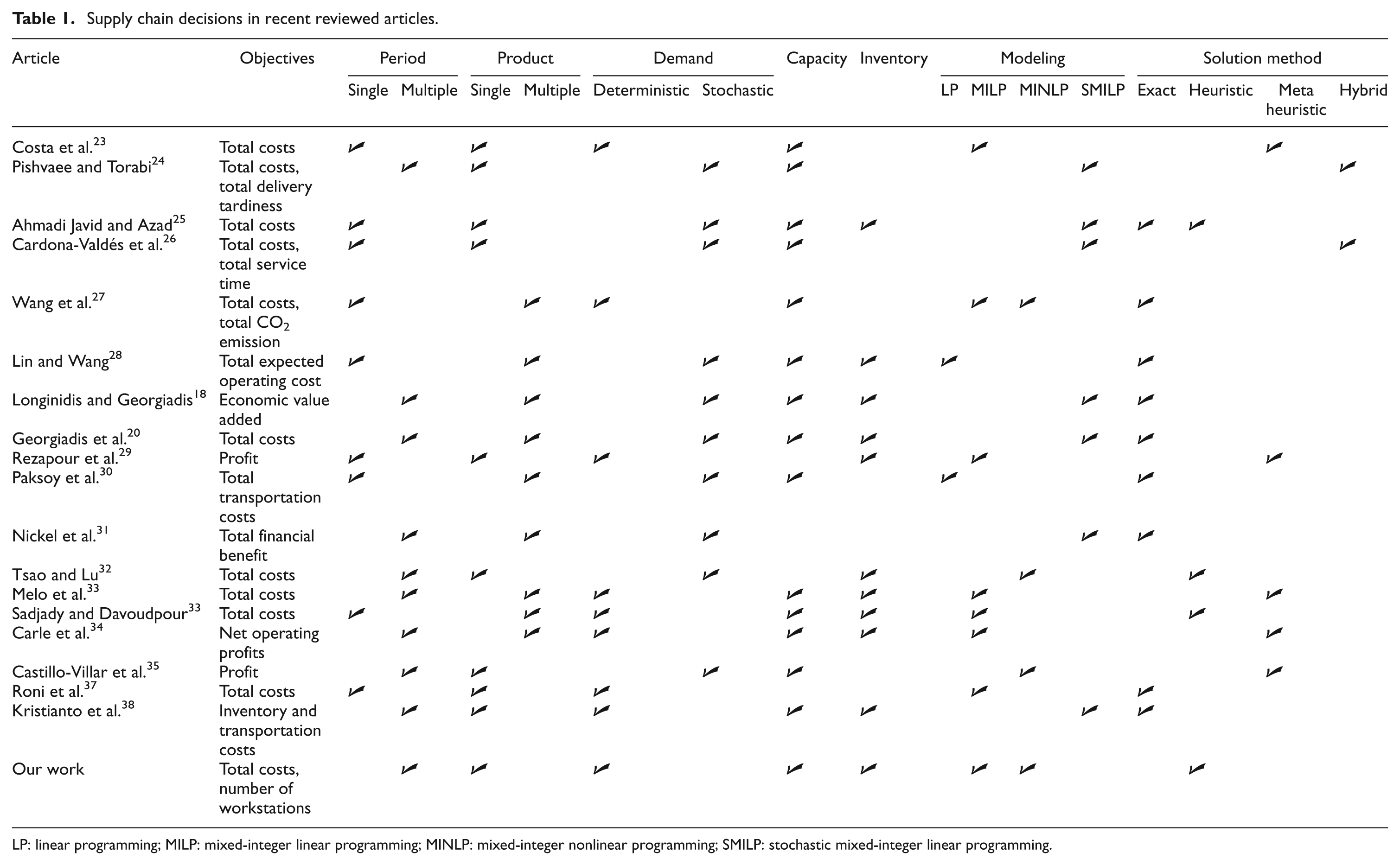
LP: linear programming; MILP: mixed-integer linear programming; MINLP: mixed-integer nonlinear programming; SMILP: stochastic mixed-integer linear programming.

Although SCND problem has been studied widely, only very little attention has been given to utilize BLP as the modeling approach. SCND problem can be represented as a Leader-Follower where top decision managers are the leaders, and the assemblers are the followers who make decisions about their activities by considering top-level decisions. Sun et al. ³⁹ present a bi-level programming model to obtain the optimal location for logistics distribution centers in which the upper-level model gives the optimal location, and the lower-level model determines an equilibrium demand distribution. Roghanian et al. ⁴⁰ address a probabilistic bi-level linear multi-objective programming problem and its application in enterprise-wide supply chain planning problem where some parameters are random variables.

ALB

After surveying studies published during the last several decades, we found that ALB problems have been addressed scarcely as a tactical decision while designing and optimizing a SCN. A traditional assembly line consists of a set of tasks, each having a certain processing time in the presence of a precedence network, which specifies the order of the tasks. In an assembly line, there are several successive workstations in which the work pieces enter the assembly line through first station and operations are carried out on them in a straight line until they reach the end of the line.^41,42 The purpose of the ALB problem is to assign tasks to the workstations in such a way that the precedence relations among tasks are not violated, and some effectiveness measures (such as cycle time, number of workstations, line efficiency or idle time) are optimized. ⁴³ In addition to straight assembly lines, the other types in the literature are U-shaped and parallel lines that depending on the final product are divided into single, mixed or multi-product lines. ⁴⁴

The simple assembly line balancing problem (SALBP) is classically classified into two major groups SALBP-I and SALBP-II and two minor groups of SALBP-E and SALBP-F. SALBP-I aims to assign tasks to workstations such that the number of workstations is minimized for a pre-specified cycle time. SALBP-II intends to minimize the cycle time, or equivalently, maximizes the production rate for a specific number of workstations. ⁴⁴ In SALBP-F, the purpose is to find a feasible task assignment for a given number of workstations and cycle time, and SALBP-E is entitled for the versions that are seeking a better line efficiency. ⁴⁵ This article focuses on a single-product and straight line with the aim of minimizing the number of workstations for a given cycle time (SALBP-I).

Problem description and formulation

In this section, at first, the basic model of BLP is introduced. Then, the basic assumptions of the problem are expressed precisely. Afterwards, the notations and the mathematical formulation are presented and the problem is extended to include push–pull strategy.

Basic model of bi-level programming

A BLP model is formulated for a problem in which two different decision-makers make decentralized decisions successively. In the problem under study in this article, SCN decisions such as flows of products and cycle times are made by top-level managers, and then determined decisions are employed in assemblers to balance the assembly lines.

BLP model has been investigated on many researches and applications up to now. ⁴⁶ In the BLP problem, each decision maker optimizes its own objective function(s) separately. However, the decisions of each level affect the decision space of other level. The general formulation of a BLP problem is as follows ⁴⁰

$$\begin{array}{c}(\mathrm{U})\underset{x}{\mathrm{Min}}F(x,y)\hfill \\ s.t.G(x,y)\le 0\hfill \\ y=y(x)\hfill \\ (\mathrm{L})\underset{y}{\mathrm{Min}}f(x,y)\hfill \\ s.t.g(x,y)\le 0.\hfill \end{array}$$

(1)

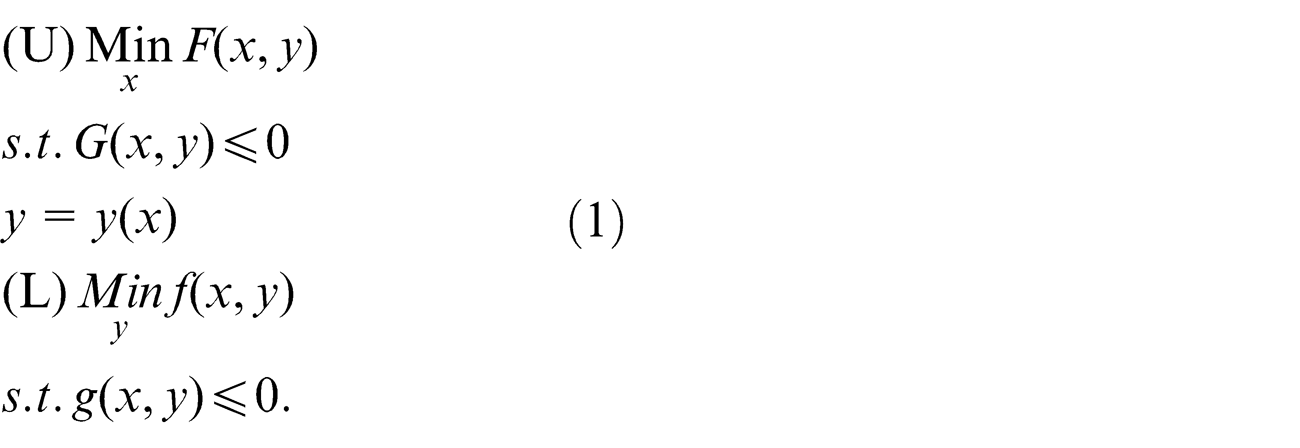
The BLP model consists of two sub-problems, (U) is defined as an upper-level problem with variables $x\in R^{n_1}$ and (L) is referred to as a lower-level problem where the decision vector of the lower-level decision-makers is $y\in R^{n_2}$ . Function $F:R^{n_1}\times R^{n_2}\to R$ is the objective function of upper-level decision-makers or top-level managers, and the vector-valued function $G:R^{n_1}\times R^{n_2}\to R^{m_1}$ is the constraint set of the upper-level decision vector. Similarly, function $f:R^{n_1}\times R^{n_2}\to R$ is the objective function of lower-level decision-makers, and $g:R^{n_1}\times R^{n_2}\to R^{m_2}$ is the constraint set of the lower-level decision vector. All of the constraints and objective functions may be linear, quadratic, nonlinear, fractional and so on. y = y(x) is commonly called reaction or response relation. ³⁹ One important key to solve the BLP model is to obtain the response function which determines the relationship between x and y variables by solving the lower-level problem and replacing the variable y in the upper-level problem. As it is clear, the response function connects the upper- and lower-level decision variables, and therefore creates dependency between two programming models.

The BLP models have much more advantages in comparison with the traditional single-level programming models. The key advantages are that (1) the BLP can be utilized to analyze two different and even conflicting objectives at the same time in the decision-making process, (2) the BLP methods can explicitly represent the mutual-action between the top-level and lower-level managers, and (3) the multiple-criteria decision-making methods of BLP can reflect the practical problem better. Since the problem under study in this article involves two different kinds of decision-makers, that is, supply chain managers and the assemblers’ decision-makers who have different objective functions, the BLP model is adopted to describe the problem appropriately.

Assumptions

The basic assumptions of the problem are characterized as follows:

1. The flow is only allowed to be transferred between two sequential echelons.

2. The customer’s demand for a product is a deterministic parameter and must be fully satisfied (shortages are not allowed).

3. The capacity of manufacturers and assemblers is pre-determined.

4. A homogenous product is assembled by performing |N| tasks of a paced serial line at most |J| workstations. It should be noted that the upper bound of the number of potential workstations can be estimated via dividing the total task times by the average cycle time.

5. Travel times of operators in workstations are ignored and work-in-process inventory is not allowed.

6. A task cannot be split among two or more workstations and all tasks must be processed.

7. The precedence relations of the problem are known, and a task cannot be accomplished until all its predecessors have been completed.

8. Each task can be assigned to only one workstation. Only one task can be processed in each workstation at a time and tasks must be processed only once.

9. The operation task time is independent of the workstation. In addition, it is not sequence-dependent.

10. The line is designed for a unique model of a single product.

The first three are usual assumptions for SCND problem, and the remaining assumptions are relevant to ALB problem in the related studies.

Mathematical model

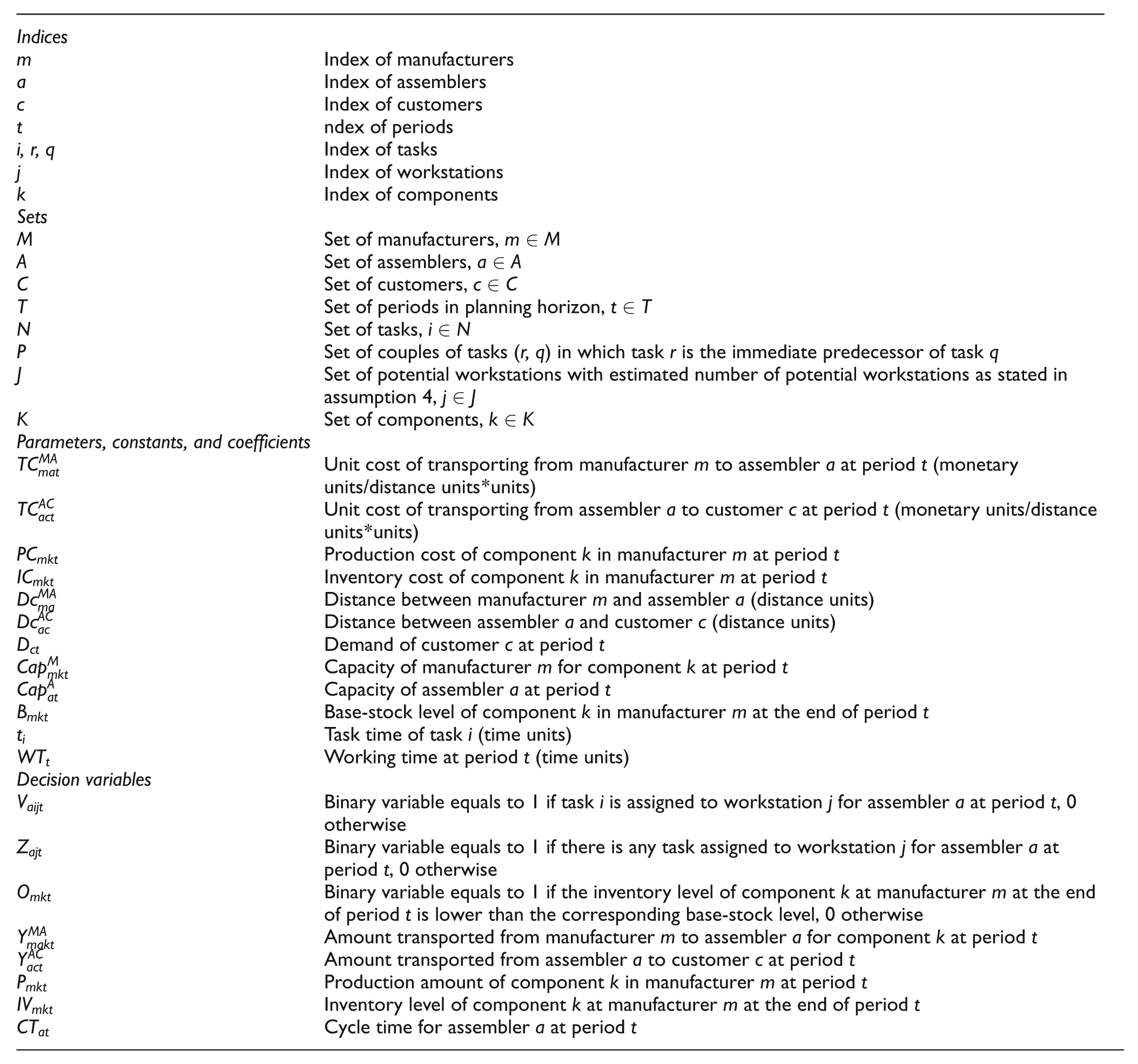
This subsection presents the BLP model of the problem. First, the upper-level model is developed. Then, the lower-level model is given. Before the introduction of mathematical formulation, indices, sets, parameters, constants and decision variables used in the model are presented as follows:

Indices
m	Index of manufacturers
a	Index of assemblers
c	Index of customers
t	ndex of periods
i, r, q	Index of tasks
j	Index of workstations
k	Index of components
Sets
M	Set of manufacturers, $m\in M$
A	Set of assemblers, $a\in A$
C	Set of customers, $c\in C$
T	Set of periods in planning horizon, $t\in T$
N	Set of tasks, $i\in N$
P	Set of couples of tasks (r, q) in which task r is the immediate predecessor of task q
J	Set of potential workstations with estimated number of potential workstations as stated inassumption 4, $j\in J$
K	Set of components, $k\in K$
Parameters, constants, and coefficients
${\mathrm{TC}}_{\mathrm{mat}}^{\mathrm{MA}}$	Unit cost of transporting from manufacturer m to assembler a at period t (monetary units/distance units*units)
${\mathrm{TC}}_{\mathrm{act}}^{\mathrm{AC}}$	Unit cost of transporting from assembler a to customer c at period t (monetary units/distance units*units)
$P{C}_{\mathrm{mkt}}$	Production cost of component k in manufacturer m at period t
$I{C}_{\mathrm{mkt}}$	Inventory cost of component k in manufacturer m at period t
${\mathrm{Dc}}_{\mathrm{ma}}^{\mathrm{MA}}$	Distance between manufacturer m and assembler a (distance units)
${\mathrm{Dc}}_{\mathrm{ac}}^{\mathrm{AC}}$	Distance between assembler a and customer c (distance units)
$D_{\mathrm{ct}}$	Demand of customer c at period t
${\mathrm{Cap}}_{\mathrm{mkt}}^M$	Capacity of manufacturer m for component k at period t
${\mathrm{Cap}}_{\mathrm{at}}^A$	Capacity of assembler a at period t
$B_{\mathrm{mkt}}$	Base-stock level of component k in manufacturer m at the end of period t
$t_i$	Task time of task i (time units)
$W{T}_t$	Working time at period t (time units)
Decision variables
$V_{\mathrm{aijt}}$	Binary variable equals to 1 if task i is assigned to workstation j for assembler a at period t, 0 otherwise
$Z_{\mathrm{ajt}}$	Binary variable equals to 1 if there is any task assigned to workstation j for assembler a at period t, 0 otherwise
$O_{\mathrm{mkt}}$	Binary variable equals to 1 if the inventory level of component k at manufacturer m at the end of period t is lower than the corresponding base-stock level, 0 otherwise
$Y_{\mathrm{makt}}^{\mathrm{MA}}$	Amount transported from manufacturer m to assembler a for component k at period t
$Y_{\mathrm{act}}^{\mathrm{AC}}$	Amount transported from assembler a to customer c at period t
$P_{\mathrm{mkt}}$	Production amount of component k in manufacturer m at period t
$I{V}_{\mathrm{mkt}}$	Inventory level of component k at manufacturer m at the end of period t
$C{T}_{\mathrm{at}}$	Cycle time for assembler a at period t

Upper-level model

In the upper-level of our developed BLP model, the SCND decisions including the amount of flows between two sequential echelons and assemblers’ cycle times are determined. It is worth mentioning that the lower-level model represents the assignment of tasks to the workstations in the assemblers

$$\begin{array}{c}\multicolumn{1}{c}{\mathrm{Min}{Z}_U={\displaystyle \sum _{m\in M}}{\displaystyle \sum _{a\in A}}{\displaystyle \sum _{k\in K}}{\displaystyle \sum _{t\in T}}{\mathrm{TC}}_{\mathrm{mat}}^{\mathrm{MA}}\times {\mathrm{Dc}}_{\mathrm{ma}}^{\mathrm{MA}}}\\ \multicolumn{1}{c}{\times Y_{\mathrm{makt}}^{\mathrm{MA}}+{\displaystyle \sum _{a\in A}}{\displaystyle \sum _{c\in C}}{\displaystyle \sum _{t\in T}}{\mathrm{TC}}_{\mathrm{act}}^{\mathrm{AC}}\times {\mathrm{Dc}}_{\mathrm{ac}}^{\mathrm{AC}}\times Y_{\mathrm{act}}^{\mathrm{AC}}}\end{array}$$

(2)

$${\displaystyle \sum _{a\in A}}{Y}_{\mathrm{makt}}^{\mathrm{MA}}\le {\mathrm{Cap}}_{\mathrm{mkt}}^M\forall m\in M,\forall k\in K,\forall t\in T$$

(3)

$${\displaystyle \sum _{c\in C}}{Y}_{\mathrm{act}}^{\mathrm{AC}}\le {\mathrm{Cap}}_{\mathrm{at}}^A\forall a\in A,\forall t\in T$$

(4)

$${\displaystyle \sum _{a\in A}}{Y}_{\mathrm{act}}^{\mathrm{AC}}\ge D_{\mathrm{ct}}\forall c\in C,\forall t\in T$$

(5)

$${\displaystyle \sum _{m\in M}}{Y}_{\mathrm{makt}}^{\mathrm{MA}}-{\displaystyle \sum _{c\in C}}{Y}_{\mathrm{act}}^{\mathrm{AC}}=0\forall a\in A,\forall k\in K,\forall t\in T$$

(6)

$$C{T}_{\mathrm{at}}\le W{T}_t/{\displaystyle \sum _{c\in C}}{Y}_{\mathrm{act}}^{\mathrm{AC}}\forall a\in A,\forall t\in T$$

(7)

$$\begin{array}{c}\multicolumn{1}{c}{Y_{\mathrm{makt}}^{\mathrm{MA}},Y_{\mathrm{act}}^{\mathrm{AC}},C{T}_{\mathrm{at}}\ge 0\forall m\in M,\forall a\in A,}\\ \multicolumn{1}{c}{\forall k\in K,\forall t\in T,\forall c\in C}\end{array}$$

(8)

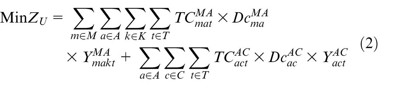
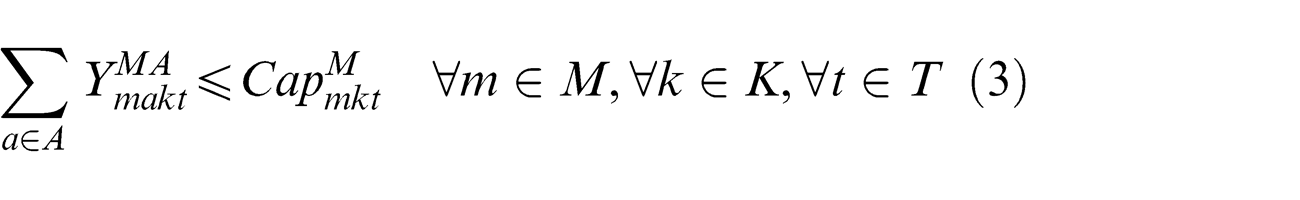
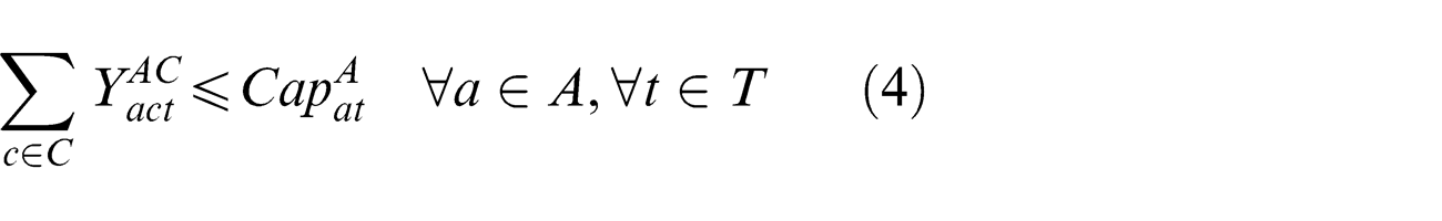
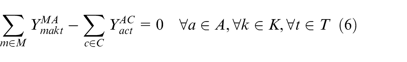
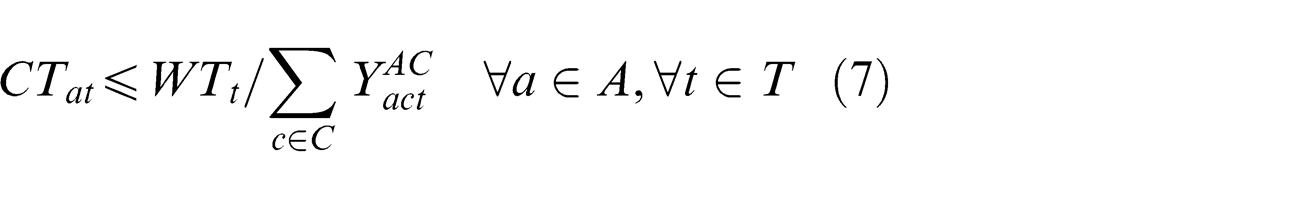
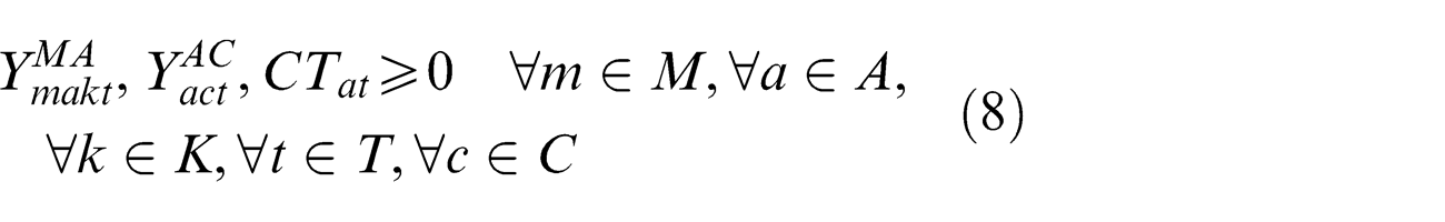
Relation (2) is the objective function of upper-level model that minimizes the sum of the transportation costs between two sequential echelons. Constraints (3) and (4) ensure the total quantity of components transported from each manufacturer to assemblers, and the total quantity of products transported from each assembler to customers cannot exceed the capacity of that manufacturer and assembler at each period, respectively. Constraint (5) guarantees the satisfaction of customer demand for all products at each period. Constraint (6) states that the total component quantity transported from manufacturers to the assembler must be equal to the total transported product quantity from that assembler to customers to satisfy the demand at each period. Constraint (7) shows that the cycle time of all assemblers at each period must be lower than or equal to the working time in all periods divided by the total product quantity required to be transported from each assembler to customers. Constraint (8) denotes the non-negativity restriction of upper-level decision variables, that is, $Y_{\mathrm{makt}}^{\mathrm{MA}}$ , $Y_{\mathrm{act}}^{\mathrm{AC}}$ and $C{T}_{\mathrm{at}}$ . As it can be seen, the upper-level model developed in this subsection is a MINLP, which can be solved by the branch-and-bound method.

Lower-level model

In the lower-level of our developed BLP model, the ALB decisions are made

$$\mathrm{Min}{Z}_L={\displaystyle \sum _{a\in A}}{\displaystyle \sum _{j\in J}}{\displaystyle \sum _{t\in T}}{Z}_{\mathrm{ajt}}$$

(9)

$${\displaystyle \sum _{j\in J}}{V}_{\mathrm{aijt}}=1\forall a\in A,\forall i\in N,\forall t\in T$$

(10)

$$\begin{array}{c}\multicolumn{1}{c}{{\displaystyle \sum _{j\in J}}j\times V_{\mathrm{arjt}}-{\displaystyle \sum _{j\in J}}j\times V_{\mathrm{aqjt}}\le 0\forall a\in A,\forall (r,q)\in P,}\\ \multicolumn{1}{c}{\forall t\in T}\end{array}$$

(11)

$${\displaystyle \sum _{i\in N}}{t}_i\times V_{\mathrm{aijt}}\le C{T}_{\mathrm{at}}\forall a\in A,\forall j\in J,\forall t\in T$$

(12)

$${\displaystyle \sum _{i\in N}}{V}_{\mathrm{aijt}}\le M\times Z_{\mathrm{ajt}}\forall a\in A,\forall j\in J,\forall t\in T$$

(13)

$$V_{\mathrm{aijt}},Z_{\mathrm{ajt}}\in \{0,1\}\forall a\in A,\forall i\in N,\forall j\in J,\forall t\in T$$

(14)

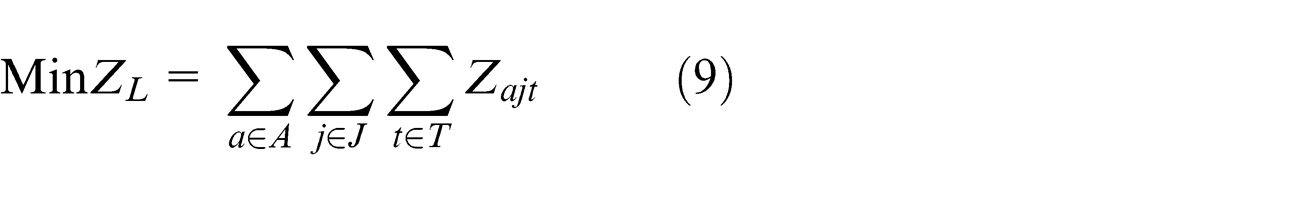
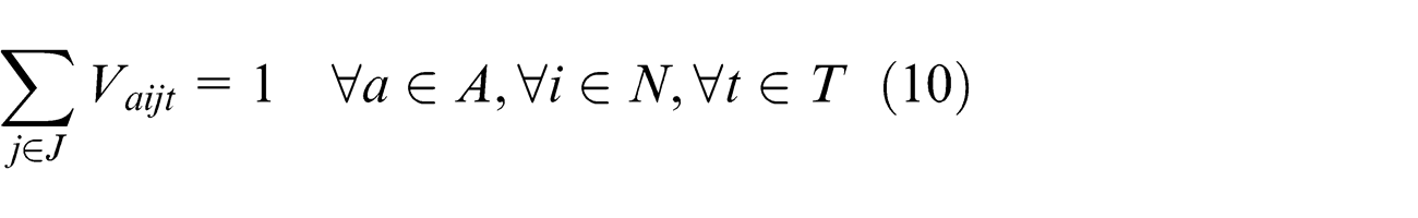
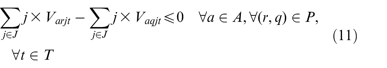
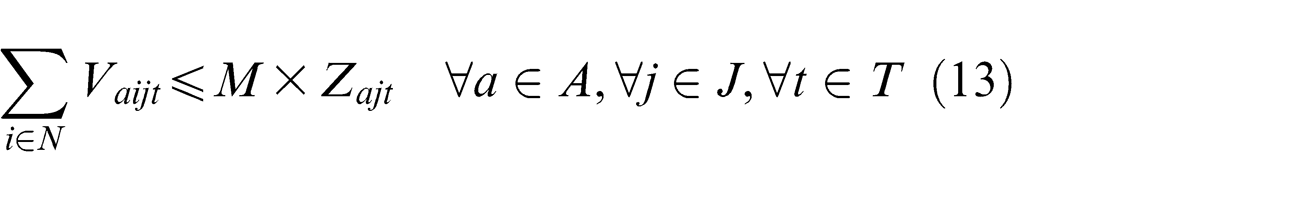
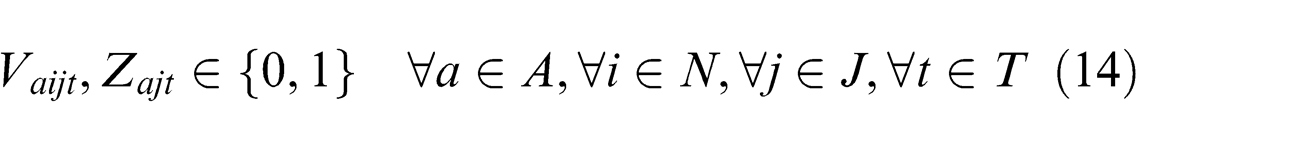
Relation (9) is the objective function of lower-level model that minimizes the total number of opened workstations in all assemblers. Constraint (10) ensures that each task is assigned to exactly one workstation in all assemblers at each period. Constraint (11) states the precedence relations between the tasks by assigning task r as an immediate predecessor of task q in all assemblers at each period. Constraint (12) guarantees that the sum of the task times in each workstation does not exceed the corresponding cycle time in all assemblers at each period. Constraint (13) ensures that station j is opened, that is, $Z_{\mathrm{ajt}}=1$ , if any task is assigned to it in all assemblers at each period. Constraint (14) expresses the binary nature of variables $V_{\mathrm{aijts}}$ and $Z_{\mathrm{ajts}}$ .

Preventing infeasibility

Based on the nature of Constraint sets (4) and (5) in the upper-level model that represent the upper and lower bounds for the amount transported from assemblers to the customers, that is, $Y_{\mathrm{act}}^{\mathrm{AC}}$ , the problem might be infeasible in some cases especially when the demand cannot be met with the available capacity. Therefore, in the following Lemma, a condition is stated to prevent the potential infeasibility in the model.

Lemma

The upper-level model presented in subsection “Upper-level model” would be feasible if the total capacity of all assemblers at each period is greater than or equal to the total demand of the customers at each period.

Proof

By rewriting Constraints (4) and (5) in the upper-level model, the following relations are obtained at each period

$$\begin{array}{c}\multicolumn{1}{c}{{\displaystyle \sum _{c\in C}}{Y}_{\mathrm{act}}^{\mathrm{AC}}\le {\mathrm{Cap}}_{\mathrm{at}}^A,\forall a\in A,\forall t\in T\to {\displaystyle \sum _{a\in A}}{\displaystyle \sum _{c\in C}}{Y}_{\mathrm{act}}^{\mathrm{AC}}}\\ \multicolumn{1}{c}{\le {\displaystyle \sum _{a\in A}}{\mathrm{Cap}}_{\mathrm{at}}^A,\forall t\in T}\end{array}$$

(15)

$$\begin{array}{c}\multicolumn{1}{c}{{\displaystyle \sum _{a\in A}}{Y}_{\mathrm{act}}^{\mathrm{AC}}\ge D_{\mathrm{ct}},\forall c\in C,\forall t\in T\to {\displaystyle \sum _{c\in C}}{\displaystyle \sum _{a\in A}}{Y}_{\mathrm{act}}^{\mathrm{AC}}}\\ \multicolumn{1}{c}{\ge {\displaystyle \sum _{c\in C}}{D}_{\mathrm{ct}},\forall t\in T}\end{array}$$

(16)

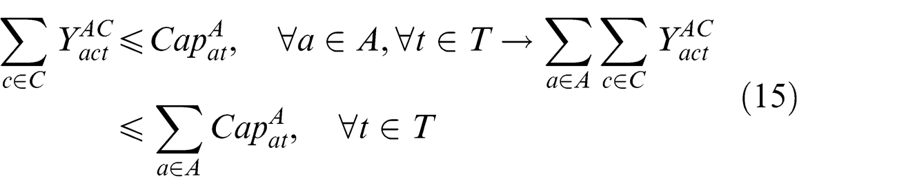
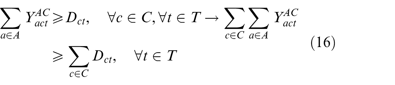
So, Constraints (15) and (16) lead to the following condition

$$\begin{array}{c}\multicolumn{1}{c}{{\displaystyle \sum _{c\in C}}{D}_{\mathrm{ct}}\le {\displaystyle \sum _{a\in A}}{\displaystyle \sum _{c\in C}}{Y}_{\mathrm{act}}^{\mathrm{AC}}\le {\displaystyle \sum _{a\in A}}{\mathrm{Cap}}_{\mathrm{at}}^A,\forall t\in T\to {\displaystyle \sum _{c\in C}}{D}_{\mathrm{ct}}}\\ \multicolumn{1}{c}{\le {\displaystyle \sum _{a\in A}}{\mathrm{Cap}}_{\mathrm{at}}^A,\forall t\in T}\end{array}$$

(17)

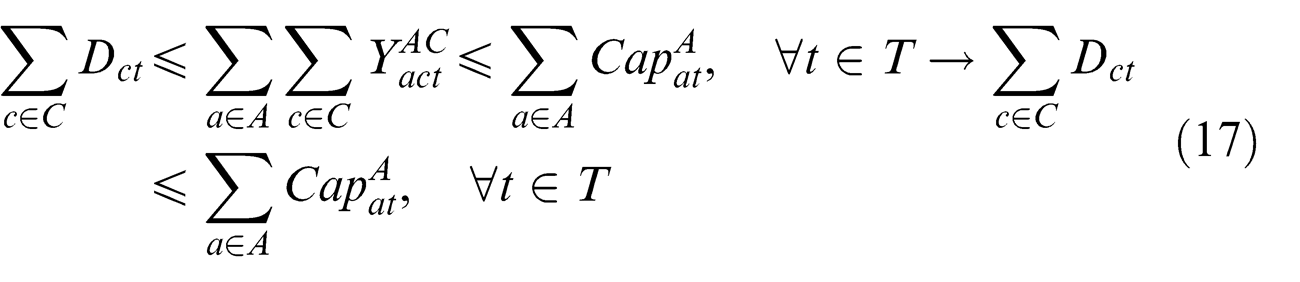
According to two constraints of the upper-level model, we found that at each period, the inequality ${\displaystyle \sum _{c\in C}}{D}_{\mathrm{ct}}\le {\displaystyle \sum _{a\in A}}{\mathrm{Cap}}_{\mathrm{at}}^A$ should be met. Inequality (17) presents that at each period, the total capacity of all assemblers should be greater than or equal to the total demand of the customers. So, if this condition is met in the problem, the upper-level model is prevented from being infeasible.

Development of push–pull strategy

Coordination of the various activities such as production, assembly, transportation and inventory decisions play an important role across a SCN. Therefore, integrating the front end to the back end of the supply chain needs to consider the different supply chain strategies. Two traditional strategies, that is, push or pull, have been employed in some previous studies.^1,47 A relatively new paradigm suggests the push–pull strategy to make production, assembly and distribution decisions.

In this subsection, we extend the problem stated in subsection “Mathematical model” to include push–pull strategy. For this purpose, the periodic review policy is used in the manufacturers in which the inventory level is reviewed at certain intervals and the appropriate amounts of components might be produced after each review. If the inventory level of component k at the end of period t is lower than the corresponding base-stock level (B_mkt ), that component is produced in manufacturer m considering its capacity in order to increase the inventory level. Employing make-to-stock approach in the manufacturers is referred to as the push-based strategy in the related literature. On the other hand, the assemblers do not hold any inventory and only respond to the customer demands using the inventory of manufacturers. This system is known as a pull-based assembled-to-order system. In other words, the developed system in this subsection includes two stages: in the first stage, components are built with a make-to-stock fashion in the manufacturers, while in the second stage, these components are assembled-to-order in response to customers’ demands. The interface between the push- and pull-based stages in the considered supply chain, that is, push–pull boundary, is illustrated in Figure 1.

Figure 1.

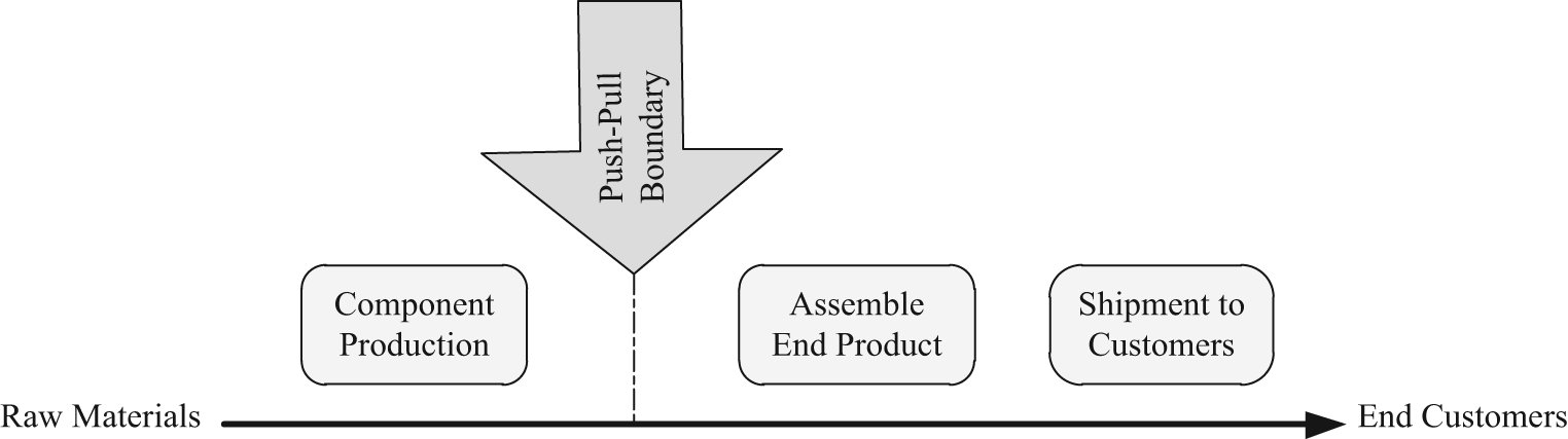
The push–pull boundary of the considered supply chain.

In order to extend the problem under study with push–pull strategy, the following relations should be added to the upper-level model presented in subsection “Upper-level model.” It is worth mentioning that the decisions such as production amount and inventory level of each component in manufacturers are also made in the upper-level model

$$\begin{array}{c}\multicolumn{1}{c}{Z{\prime }_U={\displaystyle \sum _{m\in M}}{\displaystyle \sum _{k\in K}}{\displaystyle \sum _{t\in T}}P{C}_{\mathrm{mkt}}\times P_{\mathrm{mkt}}}\\ \multicolumn{1}{c}{+{\displaystyle \sum _{m\in M}}{\displaystyle \sum _{k\in K}}{\displaystyle \sum _{t\in T}}I{C}_{\mathrm{mkt}}\times I{V}_{\mathrm{mkt}}}\end{array}$$

(18)

$$I{V}_{\mathrm{mkt}}-B_{\mathrm{mkt}}\le M(1-O_{\mathrm{mkt}})\forall m\in M,\forall k\in K,\forall t\in T$$

(19)

$$P_{\mathrm{mkt}}\le {\mathrm{Cap}}_{\mathrm{mkt}}^M\times O_{\mathrm{mkt}}\forall m\in M,\forall k\in K,\forall t\in T$$

(20)

$$P_{\mathrm{mkt}}\ge (B_{\mathrm{mkt}}+{\displaystyle \sum _{a\in A}}{Y}_{\mathrm{makt}}^{\mathrm{MA}})\times O_{\mathrm{mkt}}\forall m\in M,\forall k\in K,\forall t\in T$$

(21)

$$I{V}_{\mathrm{mkt}}=I{V}_{\mathrm{mk},t-1}+P_{\mathrm{mkt}}-{\displaystyle \sum _{a\in A}}{Y}_{\mathrm{makt}}^{\mathrm{MA}}\forall m\in M,\forall k\in K,\forall t\in T$$

(22)

$$I{V}_{\mathrm{mk},0}=0\forall m\in M,\forall k\in K$$

(23)

$$P_{\mathrm{mkt}},I{V}_{\mathrm{mkt}}\ge 0,O_{\mathrm{mkt}}\in \{0,1\}\forall m\in M,\forall k\in K,\forall t\in T$$

(24)

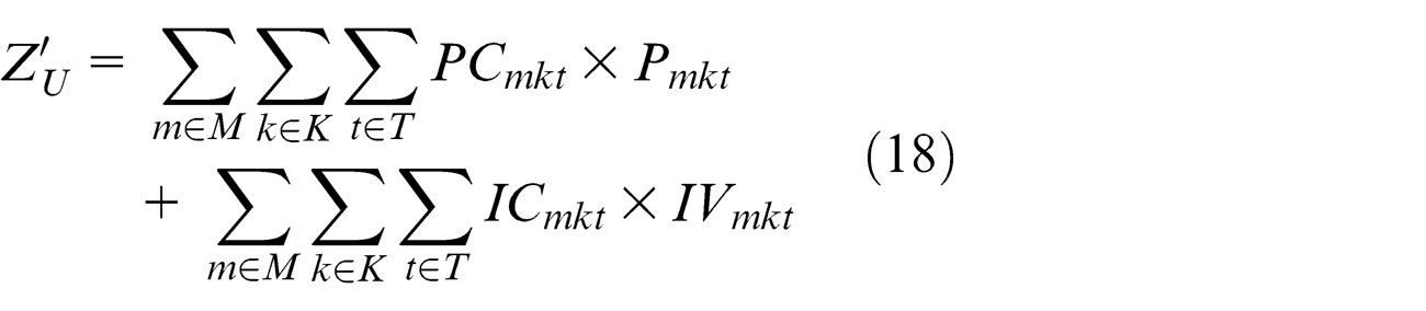
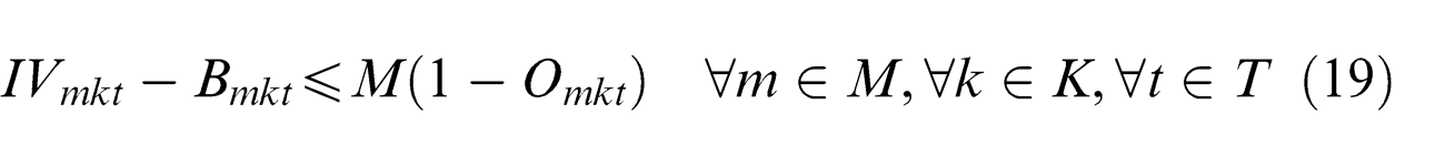
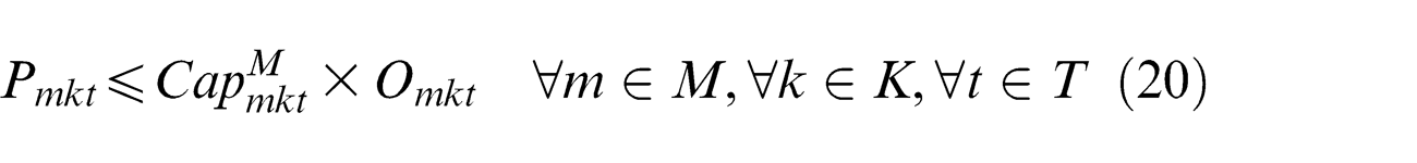
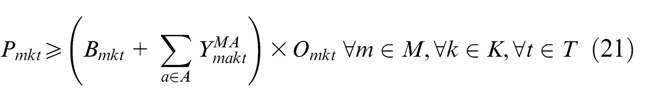
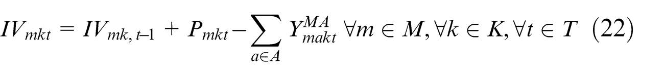
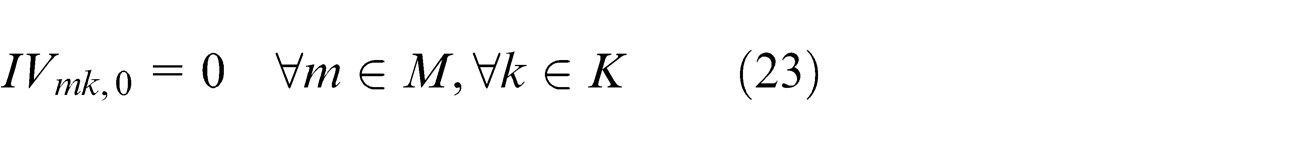
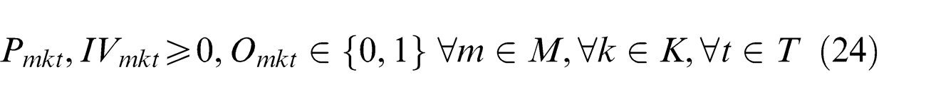
Relation (18) presents the total production and inventory costs that should be added to Relation (2) to compute the total upper-level objective function. Constraint (19) ensures that O_mkt is equal to 1 when inventory level for component k at manufacturer m at the end of period t is lower than its corresponding base-stock level. Constraint (20) guarantees that the production amount of components in each manufacturer cannot exceed the capacity of that manufacturer at each period, if O_mkt  = 1. Constraint (21) states that if component k at manufacturer m at period t is produced, that is, O_mkt  = 1, the production amount of that component must be greater than or equal to the summation of corresponding base-stock level and the outgoing flows of manufacturer m at period t. Relation (22) states that the inventory of component k at manufacturer m at the end of period t is equal to the inventory at the previous time period plus its production and minus outgoing flows. Relation (23) indicates that inventory level for component k at manufacturer m at time period 0 is equal to 0. This relation is utilized in Relation (22). Constraint (24) denotes the non-negativity restriction of new upper-level decision variables, P_mkt and IV_mkt and the binary nature of O_mkt .

Solution method

In general, it is difficult to solve the BLP problem. According to Ben-Ayed et al. ⁹ work, the BLP problem even in its simplest version is an NP-hard problem. Even if both upper and lower-level problems are convex, the whole bi-level problem is possible to be non-convex. This indicates that even if we can obtain the solution of the bi-level problem, it is generally local optimum not global optimum. The key point to solve the BLP problem is to find the response or reaction relation. As mentioned before, response relation determines the relationship between upper and lower variables in a BLP model. In view of the special form of the formulation in this article, finding relationship of upper-level variables with lower ones is simple, because Constraint (12) in the mathematical model represents explicitly the relationship between binary lower-level variables and continuous upper-level variables.

Our solution scheme in fact is a heuristic algorithm based on Constraint (12). In this method, CT_at is a given parameter in the lower-level problem. After solving the lower-level model and obtaining the value of variable V_aijt , Constraint (12) should be added to the upper-level model. Afterwards for the fixed V_aijt gained from lower-level model, upper-level problem is solved to obtain new CT_at . Since upper-level model is a MINLP problem, an appropriate solution method should be employed in each iteration such as branch-and-bound method and outer approximation algorithm. This iterative process is continued until the stopping criterion is established. The result is expected to converge into the optimal solution of the original bi-level programming model. The algorithm for the bi-level programming model is summarized as follows:

• Step 1. Determine an initial set of CT ⁰.

• Step 2. For the fixed ${\mathrm{CT}}_{\mathrm{at}}^k$ , solve the lower-level model and obtain $V_{\mathrm{aijt}}^k$ .

• Step 3. Using obtained $V_{\mathrm{aijt}}^k$ from Step 2, solve the upper-level model and obtain a new value of CT.

• Step 4. If $|Z_U^k-Z_U^{k-1}|\le \epsilon$ , stop; otherwise, set k = k + 1, go Step 2, where ε is the convergence tolerance.

Figure 2 depicts the steps of the proposed algorithm to solve the considered BLP model. It should be noted that since the upper-level model, including SCND and inventory control decisions, is an MINLP problem, it can be solved by some well-known methods. However, sometimes in order to solve it simply, an inner penalty function method can be utilized to relax nonlinear constraints, then the upper-level model could be solved by the convex combination method. ³⁹ Furthermore, because our proposed solution method is a heuristic method, it is hard to test its convergence characteristics. Therefore, different initial points can be considered to solve the problem and if all results are the same, it can be concluded that the algorithm is convergent. In addition, we can employ the mixed-integer linear programming (MILP) solution methods to solve the lower-level model, and by obtaining the response relation, the upper-level model can be solved by well-known methods that their convergence has been proved.

Figure 2.

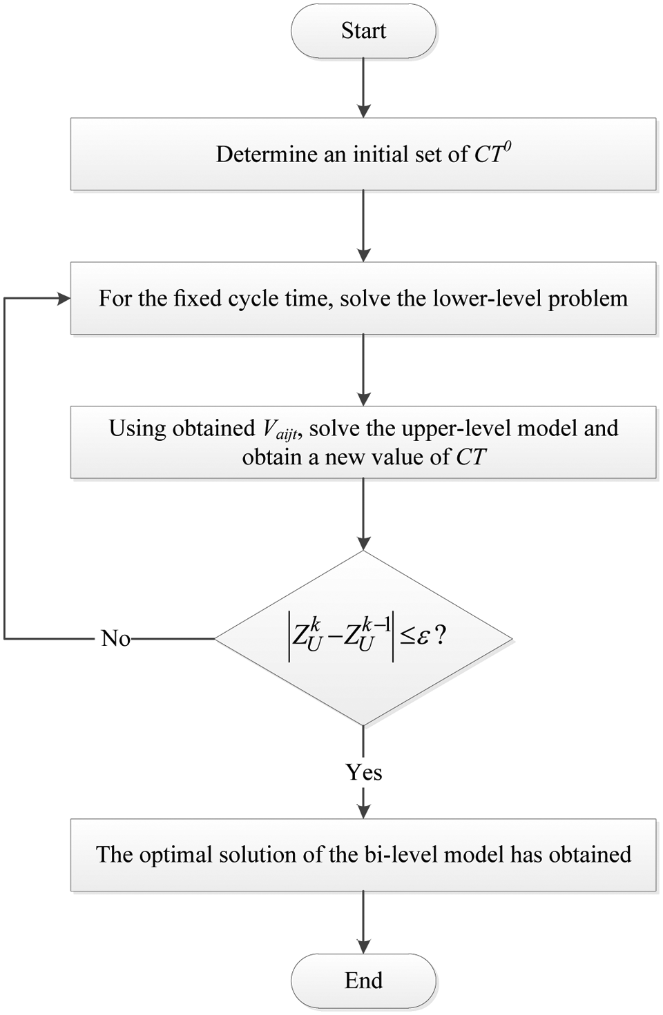
The steps of the proposed algorithm to solve the developed BLP model.

An illustrative numerical example

This subsection evaluates the developed model with a simple example using a hypothetical data set. The considered supply chain contains four manufacturers, two assemblers and four customers at shown in Figure 3. In addition to determining the transportation amounts between manufacturers, assemblers and customers, the model attempts to balance the assembly lines in assemblers simultaneously. In the assemblers, straight and single assembly lines are concerned. An example of these lines has been depicted in Figure 4.

Figure 3.

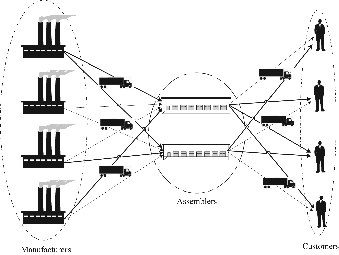
The considered supply chain network in numerical example.

Figure 4.

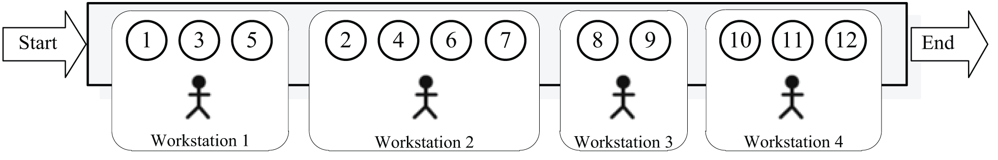
A straight and single assembly line.

Manufacturers produce seven different components and transport them to assemblers to produce end-products. After completing the assemble processes in assemblers, end-products are sent to customers. As it was mentioned, the cycle time is set fixed in the lower-level model and after determining the decision variables of this model, the new cycle time is obtained in the upper-level model. The lower-level model determines the assignment of tasks to the workstations in assemblers while the upper-level model attempts to find how many components will be transported from manufacturers to assemblers and in addition how many end-products will be sent from assemblers to customers.

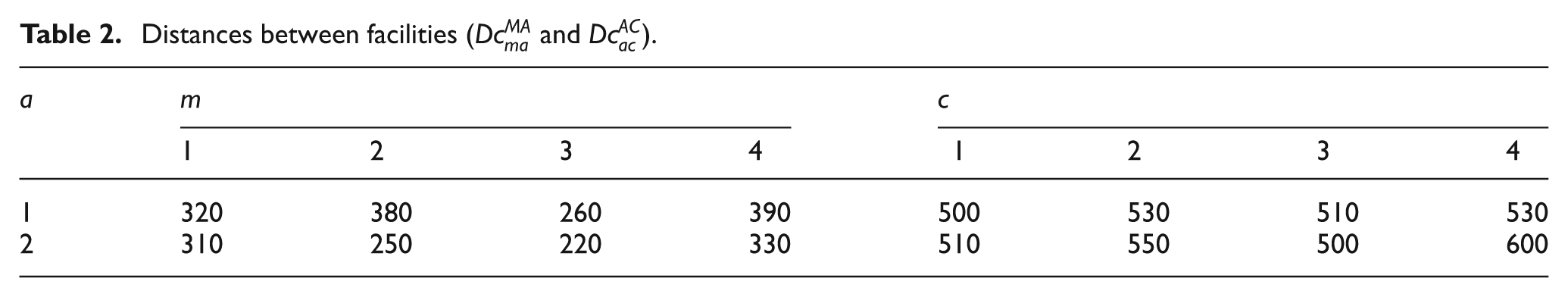
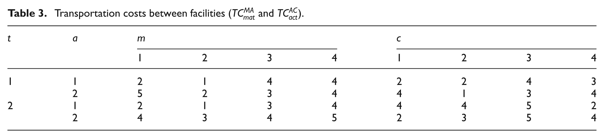
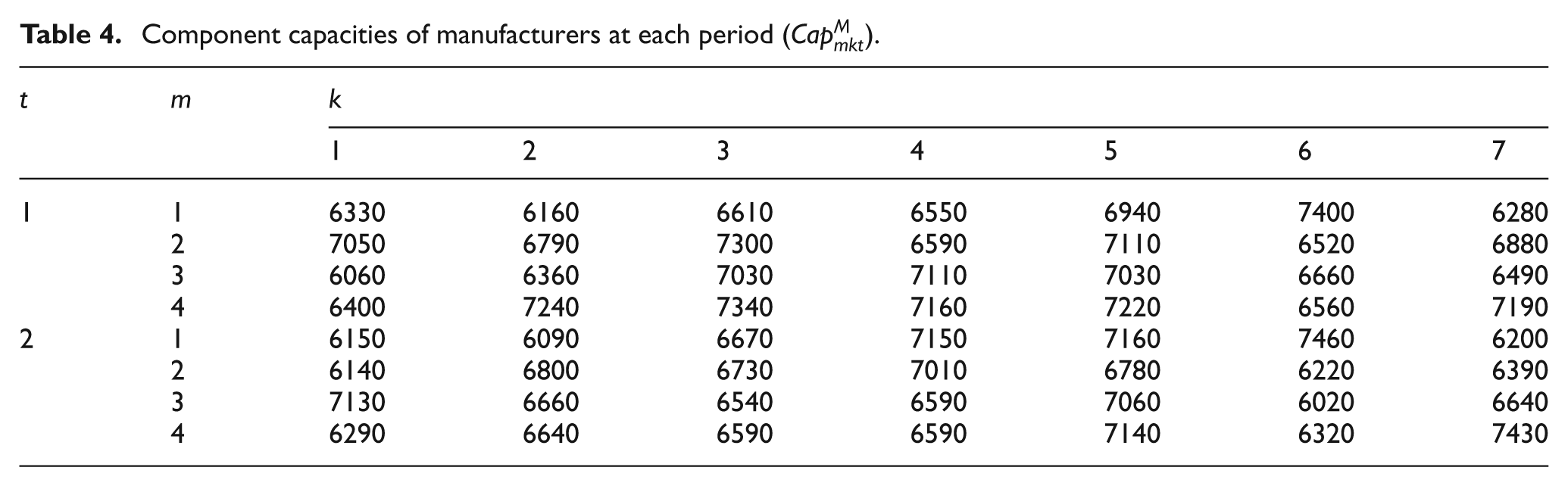
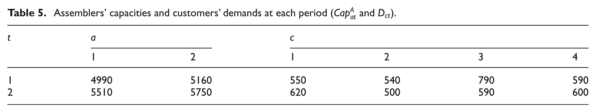
Required data for assembly lines of the assemblers are taken from the well-known web site of assembly line optimization research (www.assembly-line-balancing.de). Figure 5 demonstrates the precedence graph of the considered problem with 9 tasks in which seven different components are assembled in the assemblers. As it is seen in this figure, the numbers in the circles are task numbers while the numbers above the circles in the precedence graph are task times, which are between 1 and 6 time units. Tables 2 and 3 report the distances and unit transportation costs between facilities, respectively. Tables 4 and 5 present the capacities and demands of each facility. Two periods are considered where each period is assumed 3 months (12 weeks) with 5 working days per week and 8 working hours per day. Hence, $W_t=12\times 5\times 8\times 60=28,800min$ . Data related to the numerical example are |M| = 4, |A| = 2, |C| = 4, |T| = 2, |N| = 9, |K| = 7, |J| = 4, W_t  = 28,800 min, and the set of tasks that precedes from a task (P) are (1,2), (1,3), (2,4), (3,4), (4,5), (4,6), (4,7), (5,8), (6,9), and (7,9). The developed BLP model takes about 510 s to solve. The main results obtained from upper-level and lower-level models are reported in Tables 6 and 7, respectively. These results show the performance of the developed model and the proposed solution method in solving a simple numerical example. Table 6 gives the amount of flows between echelons, production amount and inventory level of each component in manufacturers, while Table 7 presents binary variables equal to 1 for tasks assigned to the corresponding workstations. According to the obtained results, all customers’ demands are satisfied in addition to balancing assembly workstations in the assemblers at all periods and in total, 12 workstations are opened, that is, $Z_L=12$ . As it can be seen in Table 6 at the first period, $Y_{111}^{\mathrm{AC}}+Y_{121}^{\mathrm{AC}}=550+540=1090$ units are transported from the first assembler to the customers. In order to assemble these units in the first assembler at the first period, the optimal assembly line balance contains three workstations with CT ₁₁ = 13 min. In a similar way according to the results of Table 6, the optimal distribution amounts between the assemblers and customers at two considered periods are obtained (see Figure 6). In addition, Figure 7 depicts the layout of balanced assembly lines in assemblers at each period. As it can be seen in Figure 7, the determined cycle time as the longest workstation time in the assembly line, in assemblers 1 and 2 at periods 1 and 2 are equal to 13, 14, 14 and 15 respectively, represented as (13,14;14,15).

Figure 5.

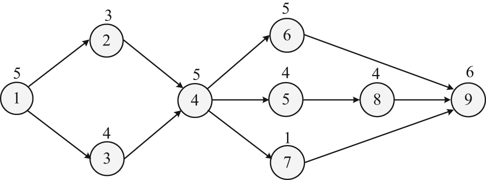
Precedence graph with the 9-task for the numerical example.

Table 2.

Distances between facilities ( ${\mathrm{Dc}}_{\mathrm{ma}}^{\mathrm{MA}}$ and ${\mathrm{Dc}}_{\mathrm{ac}}^{\mathrm{AC}}$ ).

a	m				c
	1	2	3	4	1	2	3	4
1	320	380	260	390	500	530	510	530
2	310	250	220	330	510	550	500	600

Table 3.

Transportation costs between facilities ( ${\mathrm{TC}}_{\mathrm{mat}}^{\mathrm{MA}}$ and ${\mathrm{TC}}_{\mathrm{act}}^{\mathrm{AC}}$ ).

t	a	m				c
		1	2	3	4	1	2	3	4
1	1	2	1	4	4	2	2	4	3
	2	5	2	3	4	4	1	3	4
2	1	2	1	3	4	4	4	5	2
	2	4	3	4	5	2	3	5	4

Table 4.

Component capacities of manufacturers at each period ( ${\mathrm{Cap}}_{\mathrm{mkt}}^M$ ).

t	m	k
		1	2	3	4	5	6	7
1	1	6330	6160	6610	6550	6940	7400	6280
	2	7050	6790	7300	6590	7110	6520	6880
	3	6060	6360	7030	7110	7030	6660	6490
	4	6400	7240	7340	7160	7220	6560	7190
2	1	6150	6090	6670	7150	7160	7460	6200
	2	6140	6800	6730	7010	6780	6220	6390
	3	7130	6660	6540	6590	7060	6020	6640
	4	6290	6640	6590	6590	7140	6320	7430

Table 5.

Assemblers’ capacities and customers’ demands at each period ( ${\mathrm{Cap}}_{\mathrm{at}}^A$ and $D_{\mathrm{ct}}$ ).

t	a		c
	1	2	1	2	3	4
1	4990	5160	550	540	790	590
2	5510	5750	620	500	590	600

Table 6.

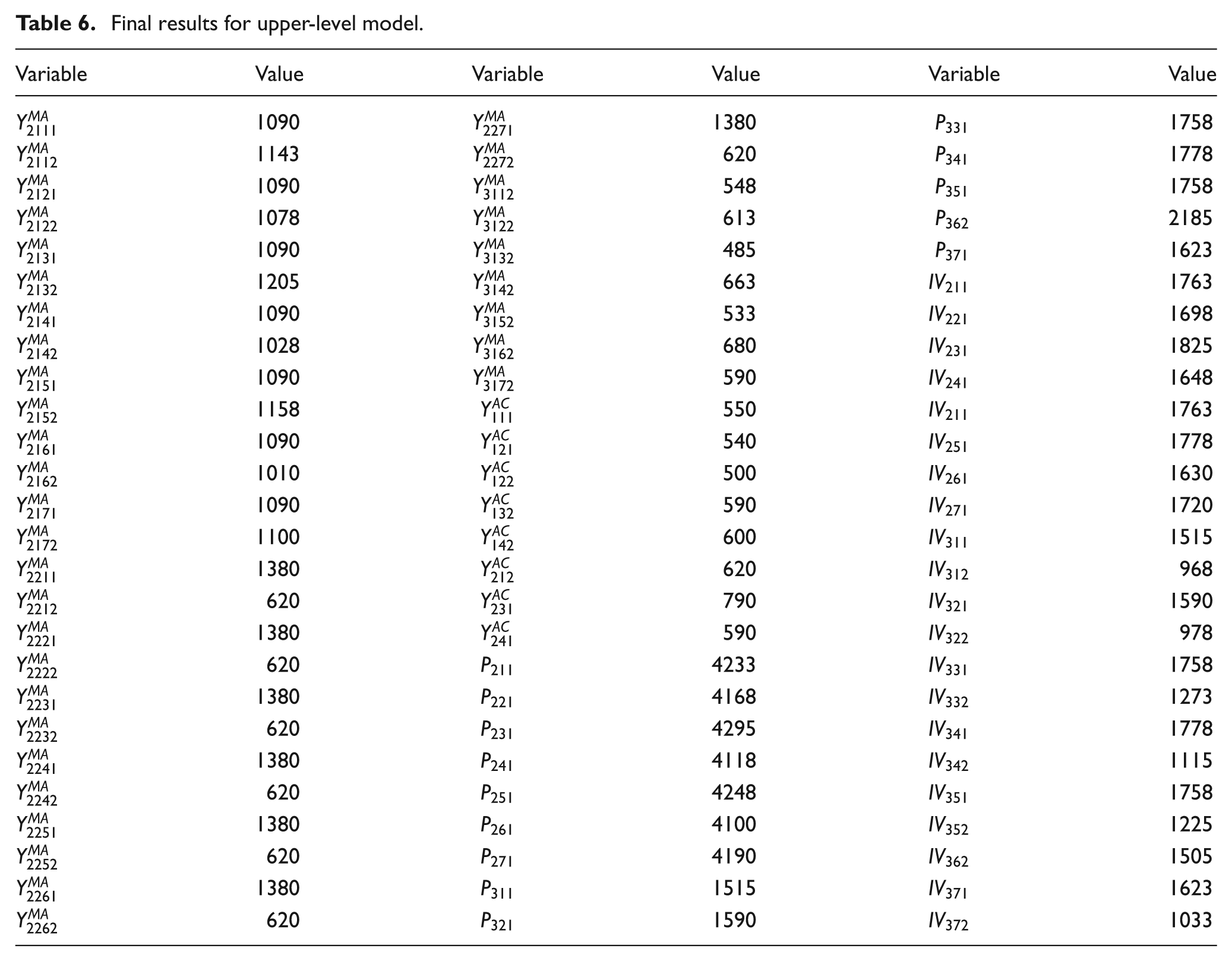
Final results for upper-level model.

Variable	Value	Variable	Value	Variable	Value
$Y_{2111}^{\mathrm{MA}}$	1090	$Y_{2271}^{\mathrm{MA}}$	1380	$P_{331}$	1758
$Y_{2112}^{\mathrm{MA}}$	1143	$Y_{2272}^{\mathrm{MA}}$	620	$P_{341}$	1778
$Y_{2121}^{\mathrm{MA}}$	1090	$Y_{3112}^{\mathrm{MA}}$	548	$P_{351}$	1758
$Y_{2122}^{\mathrm{MA}}$	1078	$Y_{3122}^{\mathrm{MA}}$	613	$P_{362}$	2185
$Y_{2131}^{\mathrm{MA}}$	1090	$Y_{3132}^{\mathrm{MA}}$	485	$P_{371}$	1623
$Y_{2132}^{\mathrm{MA}}$	1205	$Y_{3142}^{\mathrm{MA}}$	663	$I{V}_{211}$	1763
$Y_{2141}^{\mathrm{MA}}$	1090	$Y_{3152}^{\mathrm{MA}}$	533	$I{V}_{221}$	1698
$Y_{2142}^{\mathrm{MA}}$	1028	$Y_{3162}^{\mathrm{MA}}$	680	$I{V}_{231}$	1825
$Y_{2151}^{\mathrm{MA}}$	1090	$Y_{3172}^{\mathrm{MA}}$	590	$I{V}_{241}$	1648
$Y_{2152}^{\mathrm{MA}}$	1158	$Y_{111}^{\mathrm{AC}}$	550	$I{V}_{211}$	1763
$Y_{2161}^{\mathrm{MA}}$	1090	$Y_{121}^{\mathrm{AC}}$	540	$I{V}_{251}$	1778
$Y_{2162}^{\mathrm{MA}}$	1010	$Y_{122}^{\mathrm{AC}}$	500	$I{V}_{261}$	1630
$Y_{2171}^{\mathrm{MA}}$	1090	$Y_{132}^{\mathrm{AC}}$	590	$I{V}_{271}$	1720
$Y_{2172}^{\mathrm{MA}}$	1100	$Y_{142}^{\mathrm{AC}}$	600	$I{V}_{311}$	1515
$Y_{2211}^{\mathrm{MA}}$	1380	$Y_{212}^{\mathrm{AC}}$	620	$I{V}_{312}$	968
$Y_{2212}^{\mathrm{MA}}$	620	$Y_{231}^{\mathrm{AC}}$	790	$I{V}_{321}$	1590
$Y_{2221}^{\mathrm{MA}}$	1380	$Y_{241}^{\mathrm{AC}}$	590	$I{V}_{322}$	978
$Y_{2222}^{\mathrm{MA}}$	620	$P_{211}$	4233	$I{V}_{331}$	1758
$Y_{2231}^{\mathrm{MA}}$	1380	$P_{221}$	4168	$I{V}_{332}$	1273
$Y_{2232}^{\mathrm{MA}}$	620	$P_{231}$	4295	$I{V}_{341}$	1778
$Y_{2241}^{\mathrm{MA}}$	1380	$P_{241}$	4118	$I{V}_{342}$	1115
$Y_{2242}^{\mathrm{MA}}$	620	$P_{251}$	4248	$I{V}_{351}$	1758
$Y_{2251}^{\mathrm{MA}}$	1380	$P_{261}$	4100	$I{V}_{352}$	1225
$Y_{2252}^{\mathrm{MA}}$	620	$P_{271}$	4190	$I{V}_{362}$	1505
$Y_{2261}^{\mathrm{MA}}$	1380	$P_{311}$	1515	$I{V}_{371}$	1623
$Y_{2262}^{\mathrm{MA}}$	620	$P_{321}$	1590	$I{V}_{372}$	1033

Table 7.

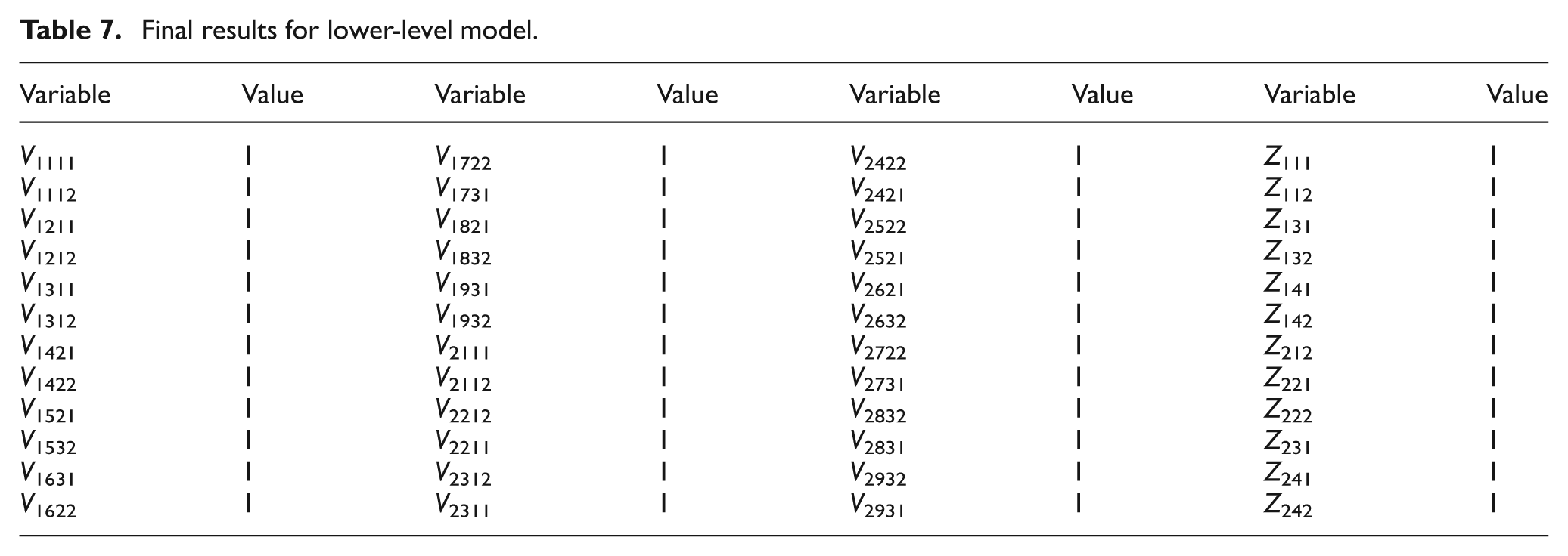
Final results for lower-level model.

Variable	Value	Variable	Value	Variable	Value	Variable	Value
V 1111	1	V 1722	1	V 2422	1	Z 111	1
V 1112	1	V 1731	1	V 2421	1	Z 112	1
V 1211	1	V 1821	1	V 2522	1	Z 131	1
V 1212	1	V 1832	1	V 2521	1	Z 132	1
V 1311	1	V 1931	1	V 2621	1	Z 141	1
V 1312	1	V 1932	1	V 2632	1	Z 142	1
V 1421	1	V 2111	1	V 2722	1	Z 212	1
V 1422	1	V 2112	1	V 2731	1	Z 221	1
V 1521	1	V 2212	1	V 2832	1	Z 222	1
V 1532	1	V 2211	1	V 2831	1	Z 231	1
V 1631	1	V 2312	1	V 2932	1	Z 241	1
V 1622	1	V 2311	1	V 2931	1	Z 242	1

Figure 6.

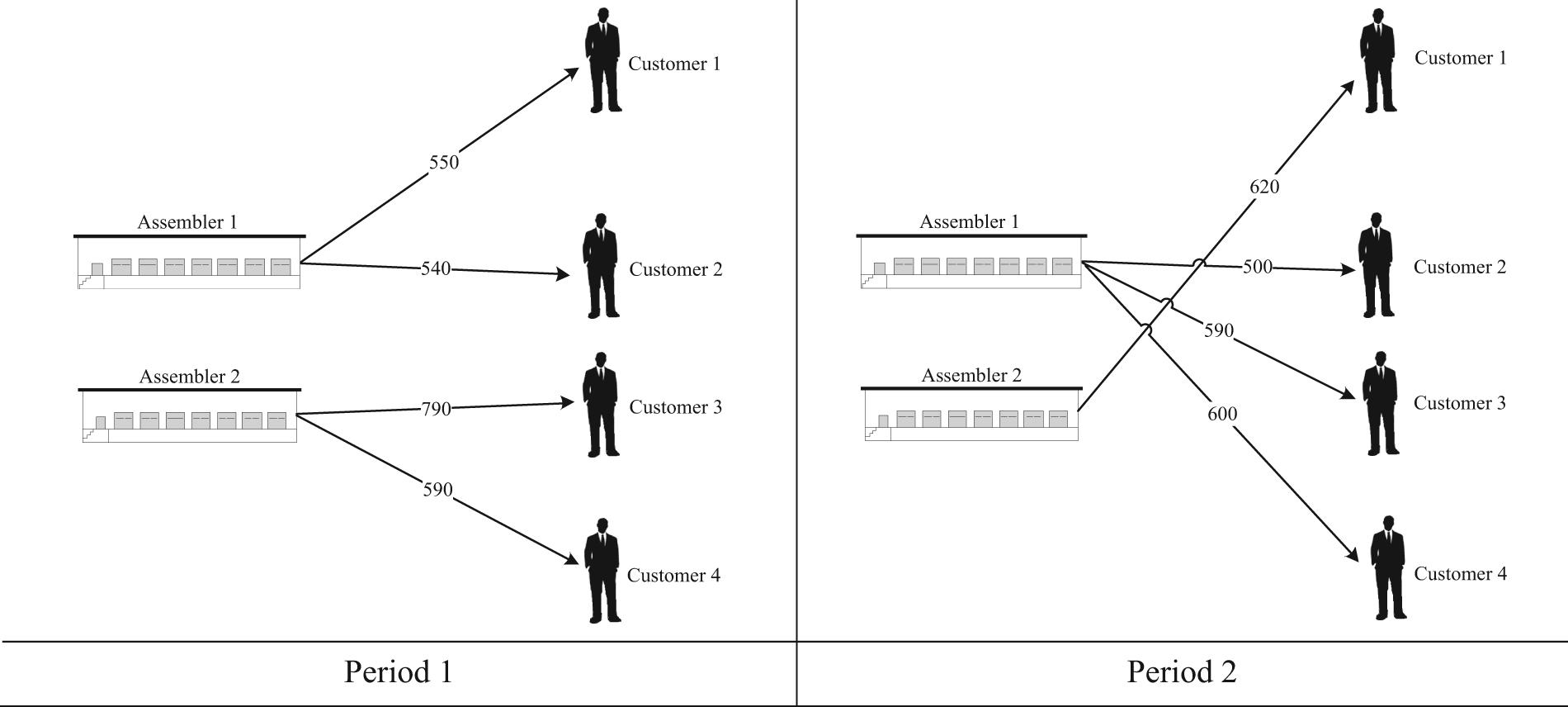
Amounts transported from the assemblers to the customers at each period.

Figure 7.

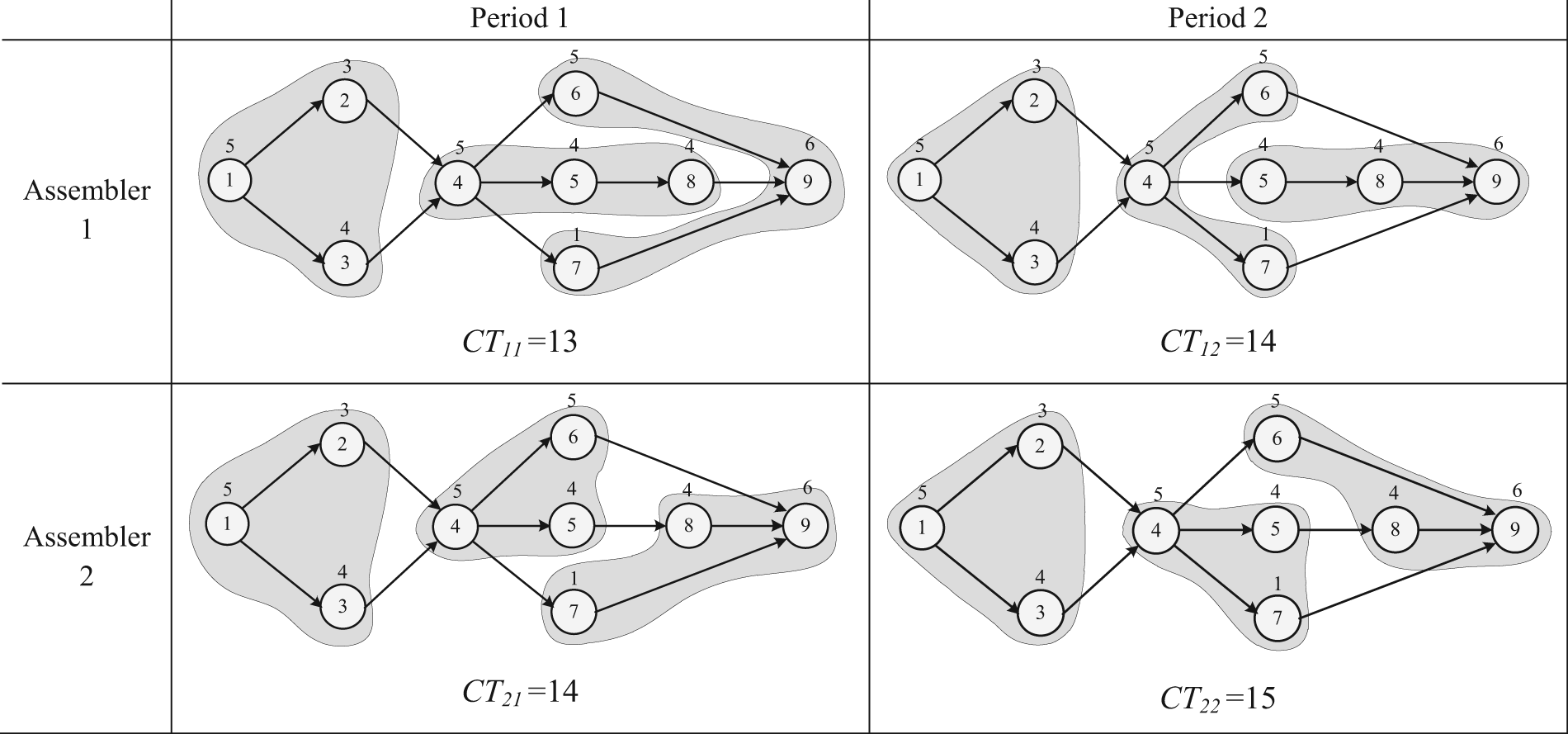
Balanced assembly diagram of assemblers at each period.

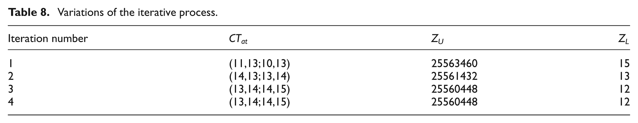
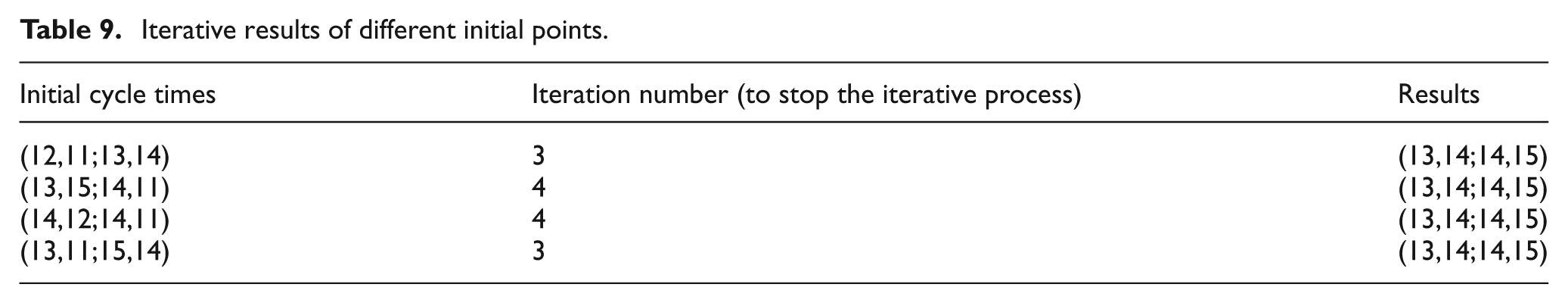
Table 8 shows the results obtained from the iterative process of the heuristic method proposed in section “Solution method” for the assemblers’ cycle time and the objective values of upper-level and lower-level models, that is, CT_at, Z_U and Z_L . Because our proposed solution method is heuristic, its convergence is difficult to be proved. However, we can solve the BLP model in the considered numerical example for several different initial cycle times in the lower-level model. If the obtained results are the same, it means the proposed solution method works well. Table 9 presents the iterative results of different initial cycle times. As it can be seen in Table 9, the solution method is convergent.

Table 8.

Variations of the iterative process.

Iteration number	$C{T}_{\mathrm{at}}$	ZU	ZL
1	(11,13;10,13)	25563460	15
2	(14,13;13,14)	25561432	13
3	(13,14;14,15)	25560448	12
4	(13,14;14,15)	25560448	12

Table 9.

Iterative results of different initial points.

Initial cycle times	Iteration number (to stop the iterative process)	Results
(12,11;13,14)	3	(13,14;14,15)
(13,15;14,11)	4	(13,14;14,15)
(14,12;14,11)	4	(13,14;14,15)
(13,11;15,14)	3	(13,14;14,15)

The solution of the numerical example presented in this subsection shows that the BLP model developed in this article is valid and useful for optimizing supply chain design and assembly lines simultaneously. While all customers’ demands are satisfied with the design of the supply chain, the assembly lines in assemblers are also balanced.

Computational experiments

This section conducts the computational experiments on a set of randomly generated test problems. The procedure used to generate these problem instances and the implementation details are explained in subsection “Problem instances generation.” Then, the computational results are reported in subsection “Computational results.”

Problem instances generation

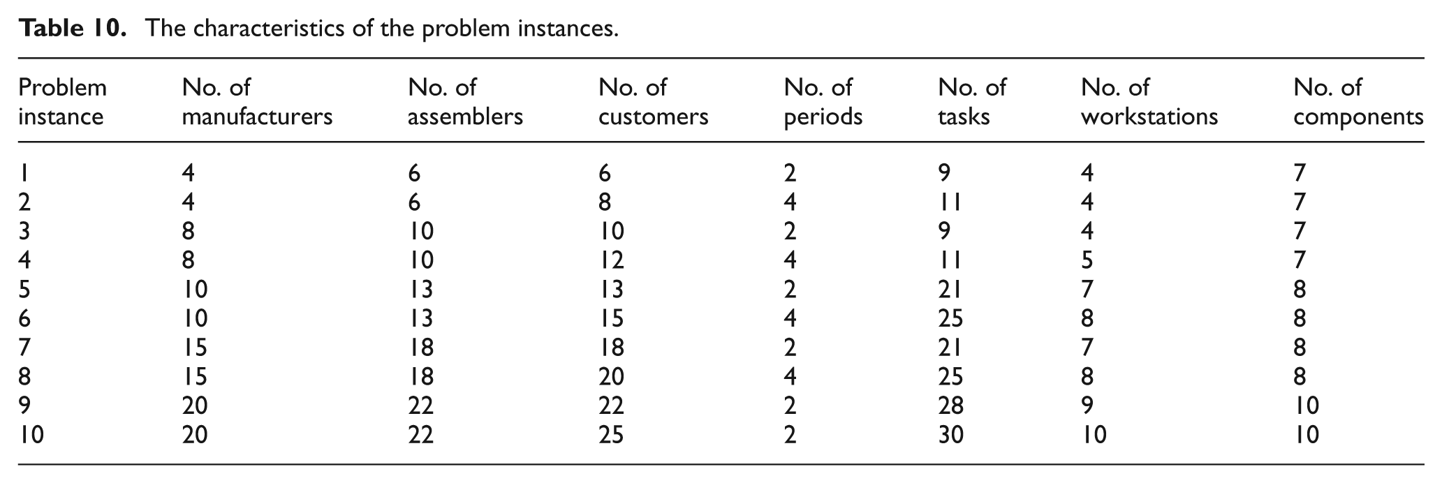
A set of problem instances is randomly generated according to assumptions that reflect the real-world situation and ease of generation and reproducibility. The size of an instance is given by the number of manufacturers (|M|), the number of assemblers (|A|), the number of customers (|C|), the number of periods (|T|), the number of tasks (|N|), the number of potential workstations (|J|), and the number of components (|K|). In this regard, the characteristics of 10 problem instances are presented in Table 10. It should be noted that the sizes of these problem instances are selected in the range of test problems provided in the recent literature. ⁶

Table 10.

The characteristics of the problem instances.

Problem instance	No. of manufacturers	No. of assemblers	No. of customers	No. of periods	No. of tasks	No. of workstations	No. of components
1	4	6	6	2	9	4	7
2	4	6	8	4	11	4	7
3	8	10	10	2	9	4	7
4	8	10	12	4	11	5	7
5	10	13	13	2	21	7	8
6	10	13	15	4	25	8	8
7	15	18	18	2	21	7	8
8	15	18	20	4	25	8	8
9	20	22	22	2	28	9	10
10	20	22	25	2	30	10	10

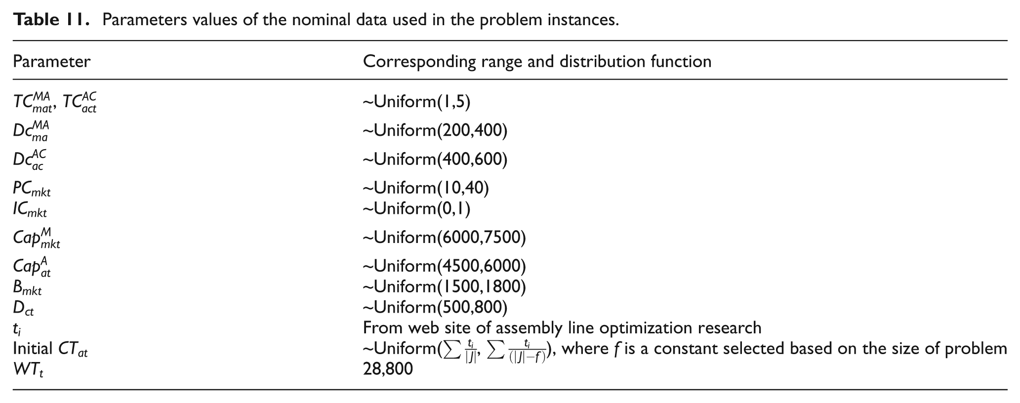
Nominal data for all problem instances are randomly generated using the distribution functions specified in Table 11. The sources of random generation for demands and capacity parameters are selected based on Lemma proved in subsection “Preventing infeasibility” to prevent infeasibility in the upper-level model. As mentioned before, the required data sets for ALB, that is, task times and precedence constraints are taken from web site of assembly line optimization research (http://www.assembly-line-balancing.de).

Table 11.

Parameters values of the nominal data used in the problem instances.

Parameter	Corresponding range and distribution function
${\mathrm{TC}}_{\mathrm{mat}}^{\mathrm{MA}}$ , ${\mathrm{TC}}_{\mathrm{act}}^{\mathrm{AC}}$	~Uniform(1,5)
${\mathrm{Dc}}_{\mathrm{ma}}^{\mathrm{MA}}$	~Uniform(200,400)
${\mathrm{Dc}}_{\mathrm{ac}}^{\mathrm{AC}}$	~Uniform(400,600)
$P{C}_{\mathrm{mkt}}$	~Uniform(10,40)
$I{C}_{\mathrm{mkt}}$	~Uniform(0,1)
${\mathrm{Cap}}_{\mathrm{mkt}}^M$	~Uniform(6000,7500)
${\mathrm{Cap}}_{\mathrm{at}}^A$	~Uniform(4500,6000)
$B_{\mathrm{mkt}}$	~Uniform(1500,1800)
$D_{\mathrm{ct}}$	~Uniform(500,800)
$t_i$	From web site of assembly line optimization research
Initial $C{T}_{\mathrm{at}}$	~Uniform( $\sum \frac{t_i}{\left|J\right|}$ , $\sum \frac{t_i}{(\left|J\right|-f)}$ ), where f is a constant selected based on the size of problem
$W{T}_t$	28,800

Computational results

This subsection presents the iteration number in which the iterative process stops, the best lower and upper objective values and the central processing unit (CPU) time for the pre-defined problems instances. It is worth mentioning that the proposed solution method was coded in MATLAB 8.0 where problem instances were formulated in GAMS on a 2.10 GHz Intel Core 2 Due CPU and 3 GB of RAM memory under Windows 7 environment. The results related to the solution of the problem instances obtained by proposed heuristic method are reported in Table 12. In addition, Figure 8 shows the convergence of the upper-level and lower-level models’ objective values (Z_U and Z_L ) for problem instances 5 and 7 until the stopping criteria is met.

Table 12.

Computational results obtained by proposed method for the defined problems instances.

Problem instance	Iteration number (to stop the iterative process)	ZU ( $\times {10}^7$ )	ZL	CPU time
1	3	2.2003	36	1380 s
2	3	6.3447	72	1589 s
3	3	3.2494	60	2295 s
4	5	10.0700	120	2641 s
5	11	5.5984	95	3433 s
6	8	10.7219	51	5342 s
7	9	6.9581	126	5206 s
8	13	11.5102	144	6427 s
9	14	7.9590	112	>3 h
10	16	8.2361	98	>3 h

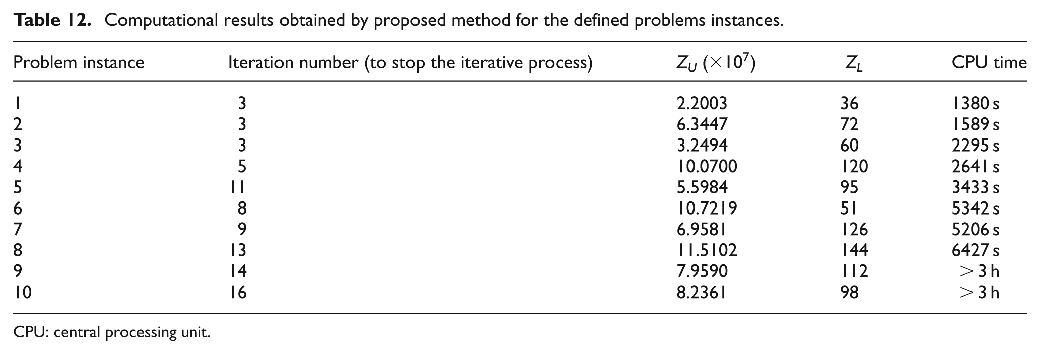
CPU: central processing unit.

Figure 8.

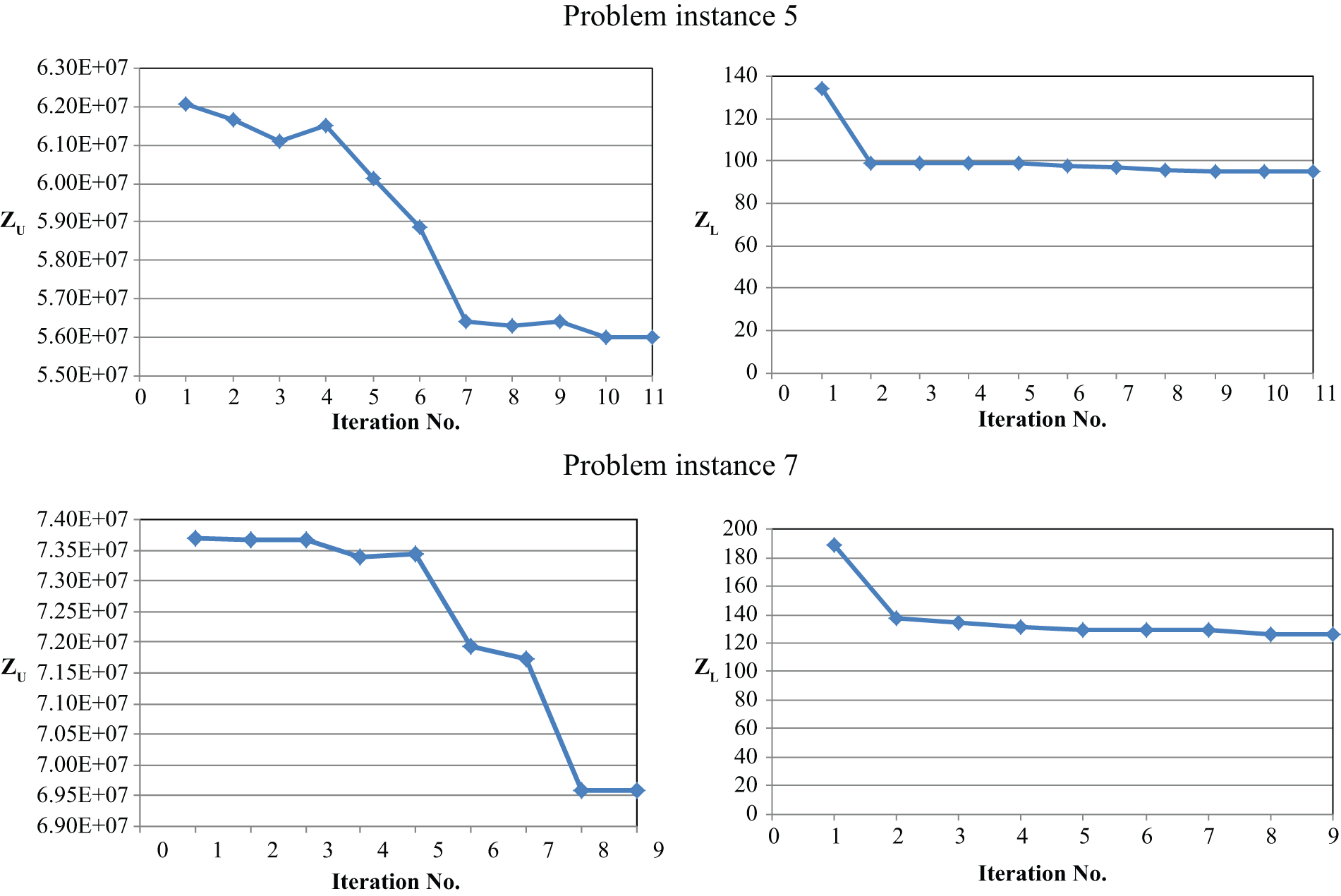
The convergence of Z_U and Z_L for problem instances 5 and 7.

Conclusion and future studies

This article tackled an important issue concerning the application of strategic and tactical decisions in SCM. The main objective of this article is to introduce and characterize the problem of integrating SCND and ALB problems. For this purpose, a SCN, including manufacturers, assemblers and customers, was considered. Due to the decentralized decisions, a novel bi-level programming model was developed to design and optimize the considered supply chain. The developed model obtains the optimum flows in the supply chain, the production amounts and the inventory levels of each component in manufacturers, and balances the assembly lines in assemblers simultaneously. In addition, a heuristic method was proposed to solve the model. Computational results on several problem instances showed that the developed model is valid and capable to be used in practical cases.

We believe this article provided a good starting point in this research area. Future research on this topic could relax some assumptions to match real-world scenarios, such as multiple products, U-shaped lines, two-sided lines, parallel stations and equipment selection. On the other hand, considering location or routing decisions in SCND problem is also a valuable future research. Furthermore, since the computational time increases significantly when problem size increases, developing an exact solution technique (e.g. benders’ decomposition or Lagrangian relaxation) or heuristic/meta-heuristic methods to solve relatively large-scale problems is a challenging area for future studies.