Dynamic study of anti-backlash gears and angle-contact ball bearing based on a simplification of the Hertz contact theory

Abstract

The contact stiffness of a mechanical joint surface has a significant influence on the assembly resonance frequency by affecting the stiffness matrix of the kinetic equation. The Hertz contact theory is improved and facilitated to found a mapping relationship between the assembly process parameters and contact stiffness, which is applied in the anti-backlash gear and the angle-contact ball bear to establish reduced model of transmission system. The anti-backlash gear can be simplified using a contact of two cylinders in reduced model, and the rotational resonance frequency of the transmission system can be increased through torsional spring preloading, while the angle-contact ball bearing can be facilitated into a contact of two spheres in reduced model, and the translational resonance frequency of the transmission system can be enhanced through axial preloading. The contact stiffness in anti-backlash gear is calculated and converted considering the driving torque and gear preloading, while the contact stiffness in angle-contact ball bearing is improved and merged by multiplying a correction factor $\xi =1.5$ in axial preloading. By adding corresponding non-massive rigid auxiliary elements, the transmission system model composed by the anti-backlash gear and the angle-contact ball bear is established to simulate the dynamic performance in ADAMS software. The frequency response values of the transmission system agree well with the theoretical value. Thus, the complex theoretical calculation formulas can be replaced by the simplified model.

Introduction

The contact interfaces between parts, components, and assemblies are called mechanical joint surfaces (joint surfaces hereafter). These interfaces belong to the flexible bodies and withstand contact pressures within a certain range. Furthermore, geometry errors, microscopic roughness, and a variety of oil mediums may exist between these interfaces. Any dynamic load will induce a slight relative linear displacement between the joint surfaces, storing and consuming energy both elastically and plastically via the contact stiffness and damping. ¹ The contact stiffness and damping of a joint surface are often a significant contributor to the overall stiffness and damping of an assembly. The studies on dynamic have demonstrated that approximately 60%−80% of the flexibility and more than 90% of the damping in an assembled body were caused by the joint surfaces.^2,3 Besides, researches on the contact stiffness and damping at a joint surface are crucial for prediction dynamics, guidance alignment, and optimization decisions for the assembly. The introduction of contact stiffness and damping at a joint surface converted a rigid couple between parts into a flexible one, which extended finite element theory from the microscale to macroscale field. In assembly body, each component was viewed as a ‘unit’, or a rigid body without any internal deformation. Deformation only occurred at the junction of a unit and another unit, namely, a ‘node’. The deformation of a unit could be replaced by one of a node. ⁴

The components are assembled according to the process sequence. The different contact states of each joint surface are determined by different assembly processes, which form the isomorphic and heterogeneous contact stiffness and damping matrices (K, C). These matrices were used to establish the kinetic equation ( $\mathbf{M}\stackrel{··}{X}+\mathbf{C}\stackrel{·}{X}+\mathbf{K}X=\mathbf{F}$ , where M, C, K, and F are mass matrix, damping matrix, stiffness matrix, and applied force vector, respectively), which would affect the dynamic characteristics of the assembly bodies. ⁵

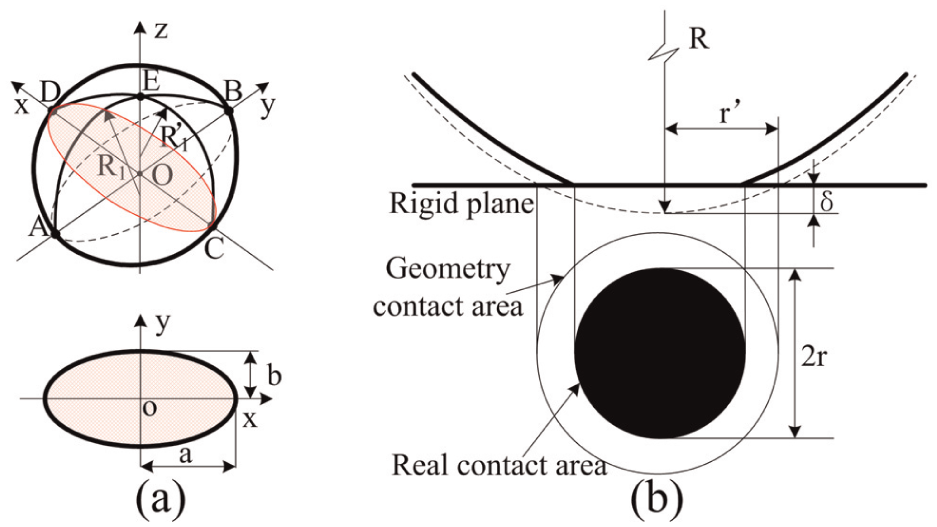
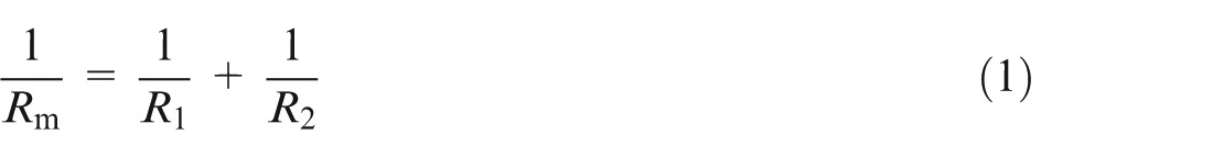
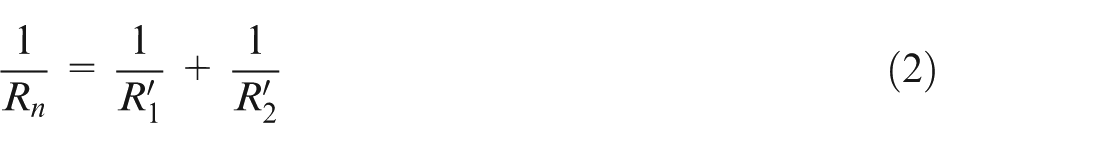
The Hertz theory^6–8 was the first method developed to solve the contact problem of frictionless elastic homogeneous surfaces with a small deformation due to normal loading. This approach yielded an index relationship between the load and area of $P~A_r^{3/2}$ , where $P$ is the load between the joint surfaces and $A_r$ is the real contact area. This relationship is solved for the contact shape, contact area, and contact stress of the contact surface, starting from the macroscopic properties of the contact body, such as the surface shape and material properties (Figure 1(a)).

Figure 1.

Hertz contact theory.

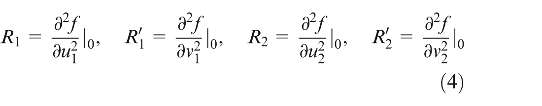
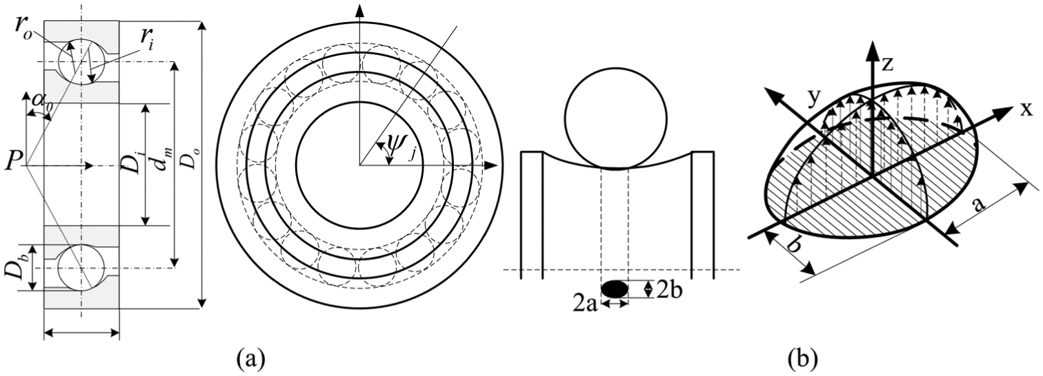
As shown in Figure 1(a), curved body I ( $w_1=f(u_1,v_1)$ , elastic modulus $E_1$ , Poisson’s ratio ${\mu }_1$ ) is in contact with curved body II ( $w_2=f(u_2,v_2)$ , elastic modulus $E_2$ , Poisson’s ratio ${\mu }_2$ ) at point E, which is called the initial point of contact. The normal surface at point E is taken as the z-axis, which can have unlimited cutting planes, including the z-axis. Each section plane intersects with a curve surface, forming an intersecting line with a different radius of curvature at point E in which there are maximum and minimum radii of curvature, referred to as the main radius and second radius of curvature, represented by $R_1$ and $R{\prime }_1$ , respectively. The direction of the two radii of curvature can be mathematically proven to be mutually perpendicular. Plane curve AEB specifies the yz plane, thus determining the positions of the x and y coordinate axes. Any contacting surfaces can be used to define a coordinate system through this method. Because the z-axis is the normal direction, when the two surfaces contact at point E, the z-axes are coincident with each other and contact area is an ellipse (Figure 1(a)).

The stress and strain between contact bodies, according to the Hertz theory, have been highly focused on and widely researched, such as the works by Tsai, ⁹ Seabra and Berthe, ¹⁰ Jackson and Streator, ¹¹ and Komvopoulos and Yang. ¹² In this article, the Hertz theory is simplified, and the contact stiffness–load relationship (derived from the load–area relationship $P~A_r^{3/2}$ ) for various of mechanical joint surfaces is explored. In addition to the Hertz theory, the Greenwood–Williamson ¹³ (G–W) contact model and Majumdar–Bhushan ¹⁴ (M–B) fractal contact model also were put forward to establish the mapping of contact stiffness–load of mechanical joint surfaces. The G–W model has been improved and modified by Pullen and Williamson, ¹⁵ Powierza et al., ¹⁶ Greenwood and Tripp, ¹⁷ Chang et al., ¹⁸ McCool and Gassel, ¹⁹ Halling and Nuri, ²⁰ and Stanley et al., ²¹ while most of them still maintained the relative simplicity of the G–W statistical representation of a surface. Other approaches based on M–B fractal models have also been developed by a number of researchers, including Majumdar and Tien, ²² Yan and Komvopoulos, ²³ and Ciavarella et al., ²⁴ where the primary basis was maintained without breaking the fractal constraint using various calculations and complicated operations. Although the precision of contact stiffness calculations has been greatly improved by the G–W and M–B models, they have some limitations in their consideration of assembly dynamic analysis. First, the roughness parameters have to be measured to calculate the contact stiffness from microscopic perspectives, which did not provide objective certainty or steady stiffness values. Second, the process was so complex and tedious that it was difficult to grasp and carry out. Third, the formulas were used repeatedly in the assembly body, which made a dynamic analysis difficult to implement. Hence, we simplified the Hertz theory to facilitate and normalize theory researches, guide the technician operations, make the alignment decision, predict the alignment performance, and optimize the alignment scheme. So if the complicated calculation and operation problems can be ignored, the Hertz’s contact theory can greatly be improved by combining with the theory of G–W and M–B.

Hertz contact model simplification

The contact between two curved bodies can be simplified by a sphere with an equivalent radius of curvature $R$ and an elastic modulus $E$ in contact with a flat rigid plane (Figure 1(b)). The radius of curvature $R$ satisfies

$$\frac{1}{R_{\mathrm{m}}}=\frac{1}{R_1}+\frac{1}{R_2}$$

(1)

$$\frac{1}{R_n}=\frac{1}{R{\prime }_1}+\frac{1}{R{\prime }_2}$$

(2)

$$R=\sqrt{R_m{R}_n}$$

(3)

$R_1,R{\prime }_1,R_2,R{\prime }_2$ as follows are the main and second radii of curvature of curved surface bodies I and II (shown Figure 1(a)), respectively. $R_m,R_n$ are the integrated main and second radii of curvature of two curved surfaces

$$R_1=\frac{{\partial }^{2}f}{\partial u_1^2}{|}_0,R{\prime }_1=\frac{{\partial }^{2}f}{\partial v_1^2}{|}_0,R_2=\frac{{\partial }^{2}f}{\partial u_2^2}{|}_0,R{\prime }_2=\frac{{\partial }^{2}f}{\partial v_2^2}{|}_0$$

(4)

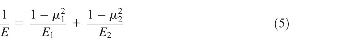
The equivalent elastic modulus $E$ is given as

$$\frac{1}{E}=\frac{1-{\mu }_1^2}{E_1}+\frac{1-{\mu }_2^2}{E_2}$$

(5)

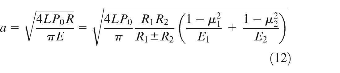
The long-half axis $a$ and short-half axis $b$ of the contact ellipse are described as $a={(3{\mathrm{FR}}_m/4E)}^{1/3},b={(3{\mathrm{FR}}_n/4E)}^{1/3}$ . From equation (3), the equivalent contact circle radius of the sphere can be obtained $r=\sqrt{\mathrm{ab}}={(3\mathrm{FR}/4E)}^{1/3}$ . The real contact area is $S=\pi R\delta =\pi r^2$ , according to the Hertz theory, where $\delta$ is the contact deformation. Set $r\prime$ as the geometry contact radius, according to the geometry restriction $\delta =R-\sqrt{R^2-r{\prime }^2}$ , namely, $2R\delta =r{\prime }^2$ due to $R>>\delta$ , so $r\prime =\sqrt{2}r$ . In Hertz theory, the contact load of the two curved surfaces $F$ has the following relationship with the deformation $\delta$

$$F=\frac{4}{3}{\mathrm{ER}}^{\frac{1}{2}}{\delta }^{\frac{3}{2}}$$

(6)

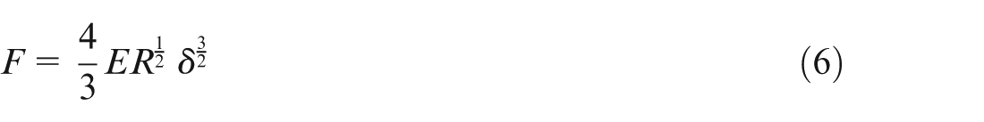
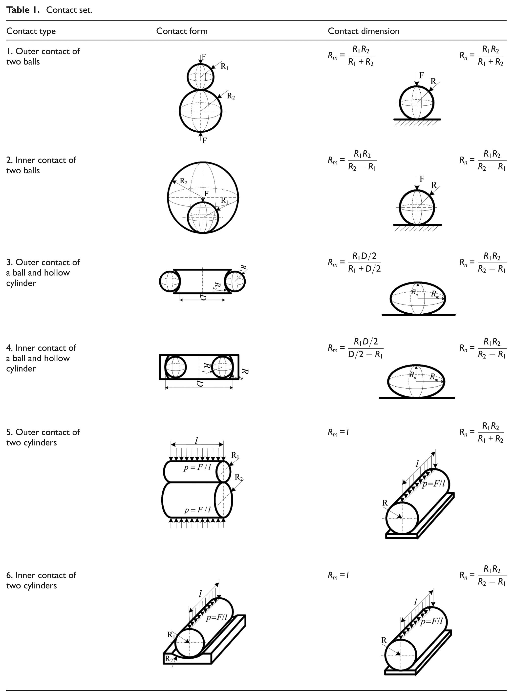
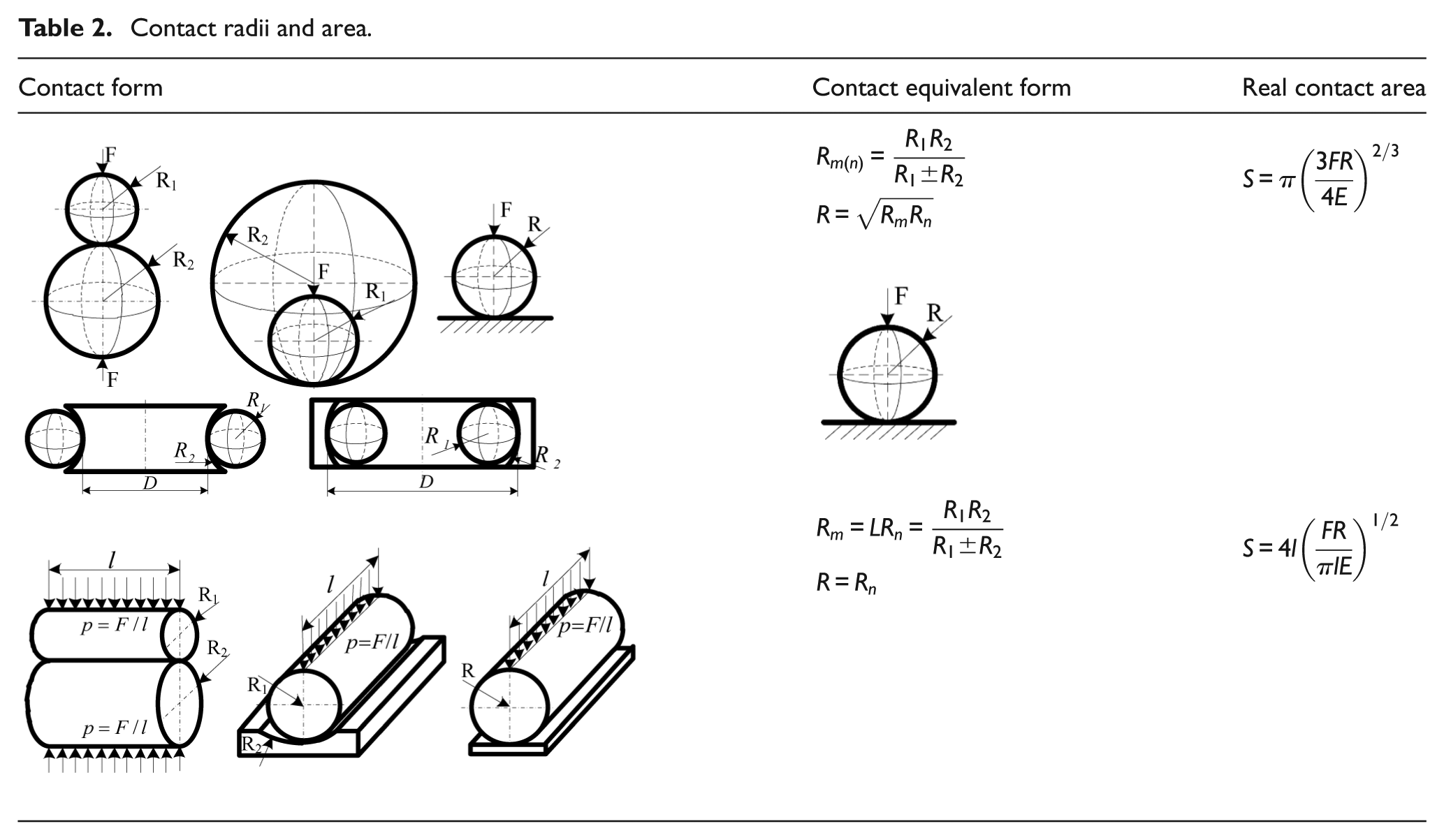
Mechanical joint surfaces are constantly changing, and thus, the corresponding contact form is complex; however, using appropriate simplifications, various mechanical joint surfaces and contact forms can be classified and simplified as shown in Tables 1 and 2. Therefore, the problem is come down to calculate the equivalent contact radius or equivalent contact area.

Table 1.

Contact set.

Contact type	Contact form	Contact dimension
1. Outer contact of two balls		$R_m=\frac{R_1{R}_2}{R_1+R_2}$	$R_n=\frac{R_1{R}_2}{R_1+R_2}$
2. Inner contact of two balls		$R_m=\frac{R_1{R}_2}{R_2-R_1}$	$R_n=\frac{R_1{R}_2}{R_2-R_1}$
3. Outer contact of a ball and hollow cylinder		$R_m=\frac{R_{1}D/2}{R_1+D/2}$	$R_n=\frac{R_1{R}_2}{R_2-R_1}$
4. Inner contact of a ball and hollow cylinder		$R_m=\frac{R_{1}D/2}{D/2-R_1}$	$R_n=\frac{R_1{R}_2}{R_2-R_1}$
5. Outer contact of two cylinders		$R_m=l$	$R_n=\frac{R_1{R}_2}{R_1+R_2}$
6. Inner contact of two cylinders		$R_m=l$	$R_n=\frac{R_1{R}_2}{R_2-R_1}$

Table 2.

Contact radii and area.

Contact form	Contact equivalent form	Real contact area
	$\begin{array}{cc}\multicolumn{1}{c}{}& R_{m(n)}=\frac{R_1{R}_2}{R_1\pm R_2}\hfill \\ \multicolumn{1}{c}{}& R=\sqrt{R_m{R}_n}\hfill \end{array}$	$S=\pi {\left(\frac{3\mathrm{FR}}{4E}\right)}^{2/3}$
	$\begin{array}{cc}\multicolumn{1}{c}{}& R_m=L{R}_n=\frac{R_1{R}_2}{R_1\pm R_2}\hfill \\ \multicolumn{1}{c}{}& R=R_n\hfill \end{array}$	$S=4l{\left(\frac{\mathrm{FR}}{\pi \mathrm{lE}}\right)}^{1/2}$

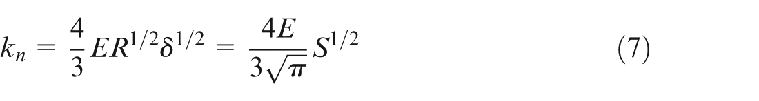
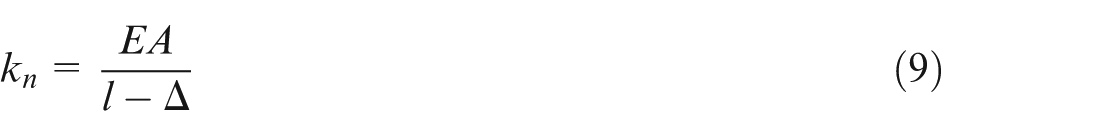
The normal contact stiffness (N/mm) is given as

$$k_n=\frac{4}{3}{\mathrm{ER}}^{1/2}{\delta }^{1/2}=\frac{4E}{3\sqrt{\pi }}{S}^{1/2}$$

(7)

where $S$ is the real contact area. The normal contact stiffness coefficient (N/mm^3/2) is

$$k_{\mathrm{nc}}=\frac{4}{3}{\mathrm{ER}}^{1/2}$$

(8)

In addition to the different radii of curvature and contact forms at the joint surface, when the contact surface is the rough plane of a bolt connection or hole–axis pairs with the same contact radius, the contact stiffness can be defined according to the following formula

$$k_n=\frac{\mathrm{EA}}{l-\Delta }$$

(9)

where $E$ is the equivalent elastic modulus of the two contact surfaces, $A$ is the nominal contact area of the two contact surfaces, and $l$ is the normal thickness of the two contact bodies. $\Delta$ has two meanings: when the rough surface of the bolt connection is in contact, $\Delta$ is the normal amount of deformation of the two contact bodies, and when the hole and axis components have the same contact radius, $\Delta$ is the amount of the overlapping tolerance zone.

The limitations of the Hertz’s contact theory: it is unable to calculate the damping coefficient between the joint surfaces. It is incapable to get the stiffness value of joint plane directly.

Contact stiffness of typical components

An anti-backlash gear improves the transmission precision of the system and the dynamic harmonic frequency by eliminating or controlling the hysteresis error, and an angle-contact ball bearing boosts the dynamic response of the support structure through axial preloading. Thus, research on corresponding dynamic models is of great significance for understanding assembly dynamic characteristics.

Contact stiffness of an anti-backlash gear

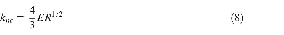
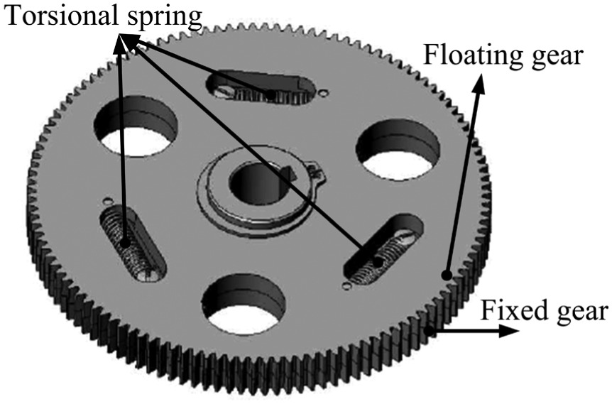
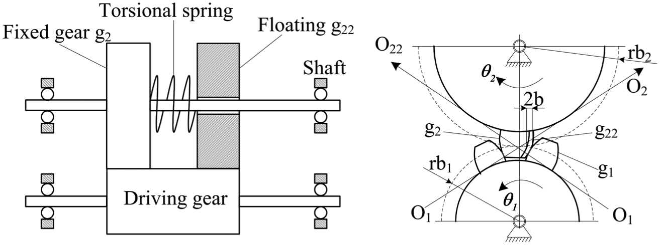
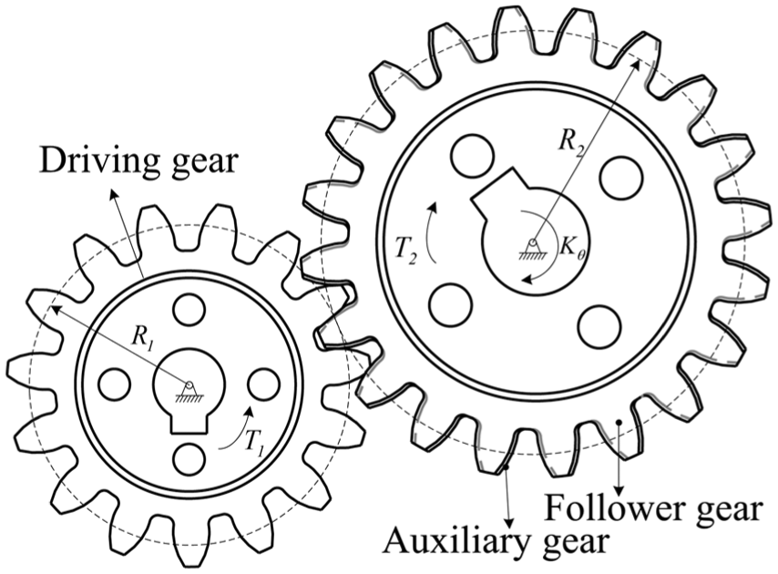
Figures 2 and 3 illustrate an anti-backlash gear, where $g_2$ is the fixed shaft gear and $g_{22}$ is a floating gear wrapped outside of the shaft which are also known as loaded gears. A torsion spring is loaded between the fixed gear and floating gear. When two gears ( $g_2$ and $g_{22}$ ) rotate a certain number of teeth relative to each other and mesh with driving gear ( $g_1$ ), the torsion spring is twisted. At this point, the teeth of gears $g_2$ and $g_{22}$ contact the two sides of driving gear $g_1$ . During working, gear $g_1$ meshes with the fixed gear $g_2$ when it rotates clockwise, and that gear $g_{22}$ is attached to the non-working side of the gear $g_1$ due to the effect of the torsion spring. When gear $g_1$ rotates anti-clockwise, it immediately meshes with gear $g_{22}$ without leaving the side vacant due to the effect of the torsion spring, thus exerting an anti-backlash effect and improving the transmission accuracy.

Figure 2.

Anti-backlash gear.

Figure 3.

Anti-backlash gear transmission.

Stiffness of the meshing at a single tooth

The contact between two involute gears can be reduced as the contact between two cylinders, as shown in Table 1, although the curvature at each point on the involute profile is not the same and the loads at various points along the working profile are different. For spur gears with a transverse contact ratio ${\epsilon }_{\alpha }$ equal to or less than 2, the contact stresses of the involute profile are very similar. Thus, both involute gears are equivalent to the outer contact of two cylinders, and the radii of the two cylinders are the pitch point curvature radii of the meshing gears.

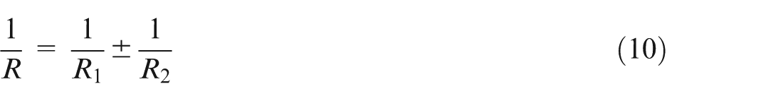
The comprehensive curvature radii of the mesh nodes are given by

$$\frac{1}{R}=\frac{1}{R_1}\pm \frac{1}{R_2}$$

(10)

where $R_1$ and $R_2$ are the pitch point curvature radii of the driving gear and anti-backlash gear, respectively. ‘+’ refers to the outer contact, and ‘−’ refers to the inner contact.

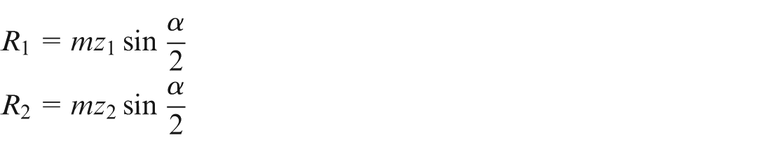
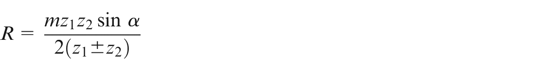
For a standard gear transmission

$$\begin{array}{c}\multicolumn{1}{c}{R_1={\mathrm{mz}}_1\sin \frac{\alpha }{2}}\\ \multicolumn{1}{c}{R_2={\mathrm{mz}}_2\sin \frac{\alpha }{2}}\end{array}$$

(11)

In the above formula, $\alpha$ refers to the pressure angle, $m$ refers to the module of the gear, and $z_1,z_2$ are the number of teeth in the driving gear and anti-backlash gear, respectively

$$R=\frac{{\mathrm{mz}}_1{z}_2\sin \alpha }{2(z_1\pm z_2)}$$

When the gears are in contact, half of the contact width can be written as

$$a=\sqrt{\frac{4{\mathrm{LP}}_{0}R}{\pi E}}=\sqrt{\frac{4{\mathrm{LP}}_0}{\pi }\frac{R_1{R}_2}{R_1\pm R_2}(\frac{1-{\mu }_1^2}{E_1}+\frac{1-{\mu }_2^2}{E_2})}$$

(12)

where $P_0$ is the contact load of a unit line, $R$ is the equivalent radius of curvature, ‘+’ is the outer contact, ‘−’ is the inner contact, $E$ is the equivalent elastic modulus, $E_1$ and $E_2$ represent the elastic moduli of the materials in the contact gears, and ${\mu }_1,{\mu }_2$ are Poisson’s ratios of the materials in the contact gears.

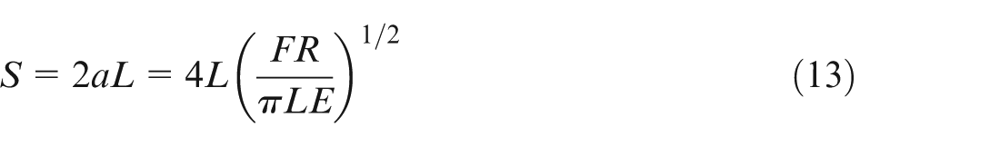
Table 2 illustrates that the gear contact area of a single tooth is

$$S=2\mathrm{aL}=4L{\left(\frac{\mathrm{FR}}{\pi \mathrm{LE}}\right)}^{1/2}$$

(13)

where $L$ refers to the contact tooth surface width given in the above formula.

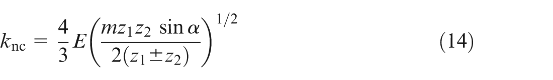
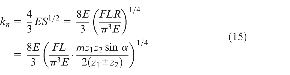
The normal contact stiffness coefficient of the gear tooth is

$$k_{\mathrm{nc}}=\frac{4}{3}E{\left(\frac{{\mathrm{mz}}_1{z}_2\sin \alpha }{2(z_1\pm z_2)}\right)}^{1/2}$$

(14)

and the normal contact stiffness of a single gear tooth is

$$\begin{array}{cc}\multicolumn{1}{c}{k_n}& =\frac{4}{3}{\mathrm{ES}}^{1/2}=\frac{8E}{3}{\left(\frac{\mathrm{FLR}}{{\pi }^{3}E}\right)}^{1/4}\hfill \\ \multicolumn{1}{c}{}& =\frac{8E}{3}{(\frac{\mathrm{FL}}{{\pi }^{3}E}·\frac{{\mathrm{mz}}_1{z}_2\sin \alpha }{2(z_1\pm z_2)})}^{1/4}\hfill \end{array}$$

(15)

Comprehensive mesh stiffness

By assuming that the stiffness of the anti-backlash torsional spring is $k_{\eta }$ , the torsion stiffness between gears $g_2$ and $g_{22}$ must also be $k_{\eta }$ , which is equivalent to a linear stiffness on the meshing line of $k_x=k_{\eta }/{\mathrm{rb}}_2^2$ , where ${\mathrm{rb}}_2$ is the pitch circle radius of gears $g_2$ and $g_{22}$ .

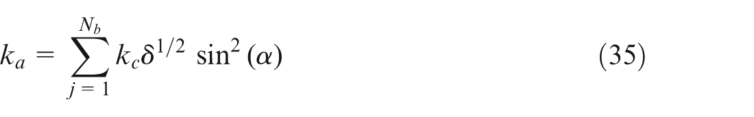
To eliminate the effects of vibration produced by gear backlash, when assembling anti-backlash gears, the anti-backlash torsional spring must be pre-biased by a certain angle $\Delta \theta =2\pi z\prime /z$ , where $z\prime$ and z are the numbers of pre-deflected teeth and total teeth, respectively. Therefore, the preload moment of the anti-backlash gear is equal to the moment produced by the torsional spring $\Delta T=k_{\eta }·\Delta \theta$ , and the preload force on the meshing line is

$$F=k_x·\Delta x=\pi k_x\mathrm{mz}\prime$$

(16)

In the above equation, $k_x$ is the linear stiffness of the torsion spring and the linear displacement is given by $\Delta x={\mathrm{rb}}_2·\Delta \theta$

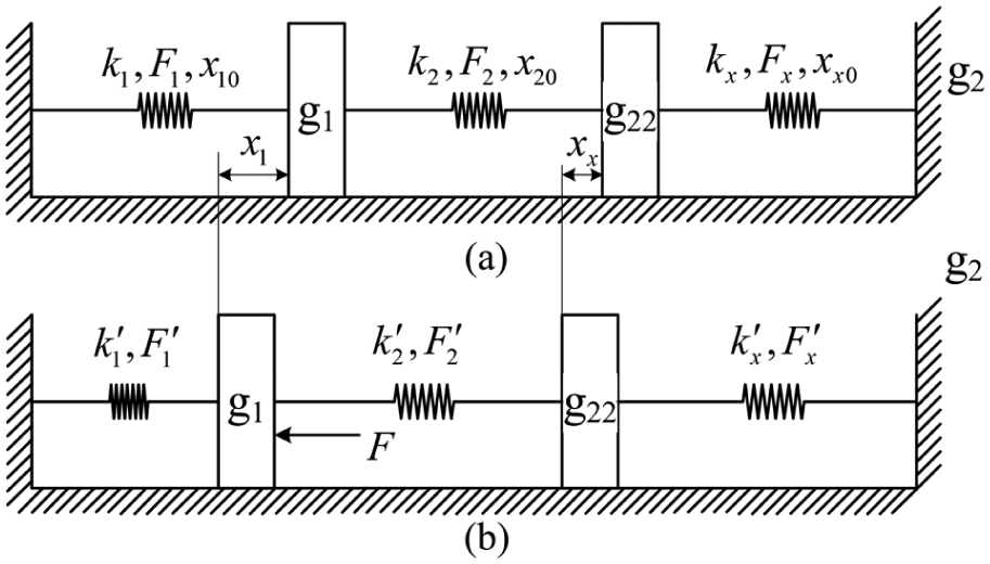
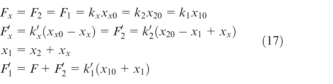
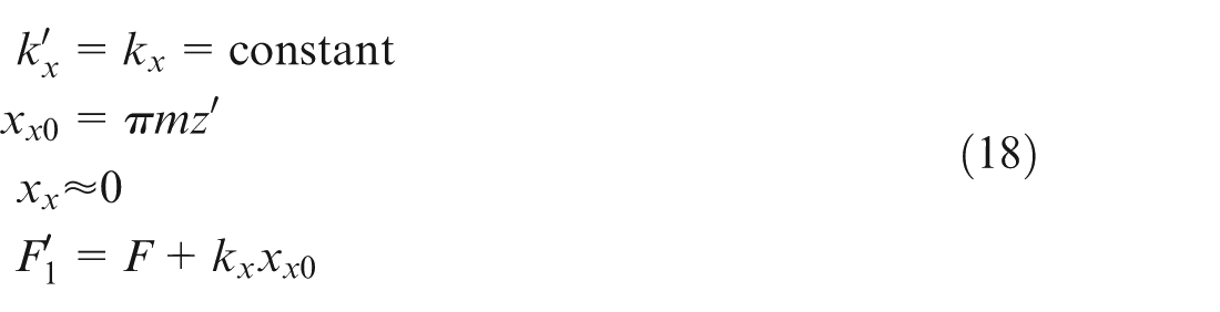
Let us set $F_1,F_2,F_x$ as the preload forces and $x_{10},x_{20},x_{x0}$ as the original linear displacement produced by torsional spring’s preload moments which is positive with compressing and negative with elongating. $k_1,k_2,k_x$ are the initial contact stiffness on the meshing lines between gears $g_1$ and $g_2$ , $g_1$ and $g_{22}$ , and $g_2$ and $g_{22}$ , respectively. $F$ is the contact force or impact force between driving gear and anti-backlash gear coming from motor torque (Figure 4).

Figure 4.

Equivalent model of anti-backlash gears: (a) preloading status and (b) working status.

Thus

$$\begin{array}{cc}\multicolumn{1}{c}{F_x}& =F_2=F_1=k_x{x}_{x0}=k_2{x}_{20}=k_1{x}_{10}\hfill \\ \multicolumn{1}{c}{F{\prime }_x}& =k{\prime }_x(x_{x0}-x_x)=F{\prime }_2=k{\prime }_2(x_{20}-x_1+x_x)\hfill \\ \multicolumn{1}{c}{x_1}& =x_2+x_x\hfill \\ \multicolumn{1}{c}{F{\prime }_1}& =F+F{\prime }_2=k{\prime }_1(x_{10}+x_1)\hfill \end{array}$$

(17)

Suppose that

$$\begin{array}{cc}\multicolumn{1}{c}{k{\prime }_x}& =k_x=\mathrm{constant}\hfill \\ \multicolumn{1}{c}{x_{x0}}& =\pi \mathrm{mz}\prime \hfill \\ \multicolumn{1}{c}{x_x}& \approx 0\hfill \\ \multicolumn{1}{c}{F{\prime }_1}& =F+k_x{x}_{x0}\hfill \end{array}$$

(18)

If $k_x=0$ , that is, there are no torsional springs, $F{\prime }_1=F$ and the anti-backlash gears are reduced to general gears. Alternatively, if $F=0$ , that is, the gears are static, $F{\prime }_1=k_x{x}_{x0}$ and the contact forces between the gears are produced by the torsional springs only.

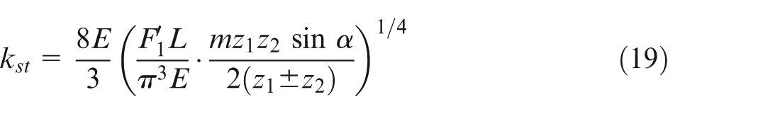
As a result, the meshing contact stiffness of the anti-backlash gears is

$$k_{\mathrm{st}}=\frac{8E}{3}{(\frac{F{\prime }_{1}L}{{\pi }^{3}E}·\frac{{\mathrm{mz}}_1{z}_2\sin \alpha }{2(z_1\pm z_2)})}^{1/4}$$

(19)

Modelling and simulation of the anti-backlash gear

In the simulation process, a non-flexible and non-massive auxiliary gear is added and forms a gear pair with the driving gear. Therefore, the driving gear is engaged with the auxiliary gear instead of the follower gear. While working, the driving gear transfers power through the virtual gear pair to the auxiliary gear and then to the follower gear through the torsional springs.

The dynamic model of the transformed gear pair is shown in Figure 5, where $R_1$ and $R_2$ are the driving and follower gears’ pitch circle radii, respectively, $k_{\theta }$ is the equivalent torsional spring stiffness, $T_1$ is the driving moment of the driving gear, and $T_2$ is the moment transferred from the virtual gear pair to the follower gear, which equals the moment transferred by the torsional spring.

Figure 5.

Dynamic simulation of anti-backlash gear.

During the transformation of the two gear pairs, the moments between the driving and follower gears, which are produced by the dynamic meshing force, are identical. Then, the equivalent torsional spring stiffness is

$$k_{\theta }=k_{\mathrm{st}}{R}_2^2$$

(20)

where $k_{\mathrm{st}}$ is the meshing contact stiffness of the anti-backlash gear and $R_2$ is the base radius of the anti-backlash gear.

Contact stiffness at the angle-contact ball bearing

An angle-contact ball bearing is composed of four major parts: an inner ring, outer ring, cage, and rolling body. The cage is an important component of a rolling bearing to keep and warranty an adequate position of its rolling bodies, but it has little impact for contact stiffness between rolling and rings, so the cage is neglected in model for convenience and the rolling bodies’ position is guaranteed by several springs which can only be compressed. While working, a rolling body produces deformations that link the inner and outer rings, which can be viewed as two springs in series. The radial components of the contact stiffness of all rolling bodies are parallel, as are the axial components.

Contact stiffness of a single rolling body

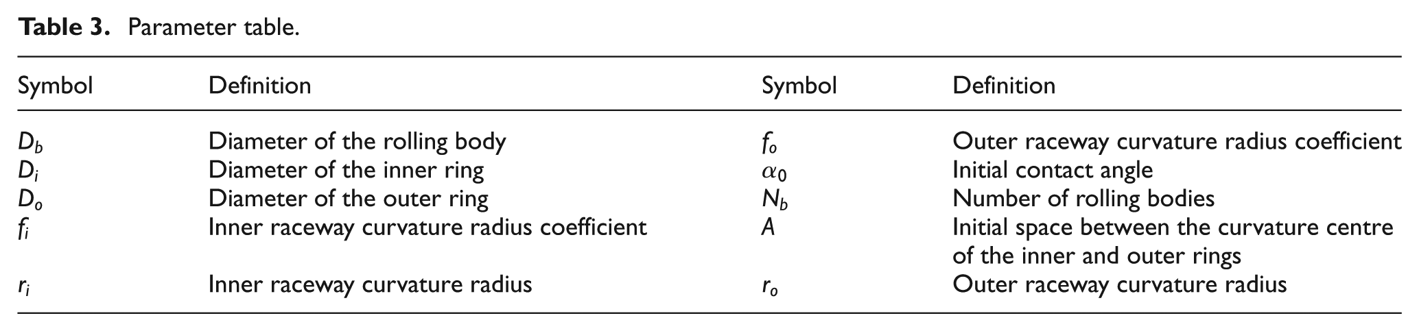
Dimensions related to the angle-contact ball bearing and the deformations between a rolling body and an inner and outer ring are shown in Figure 6, and the corresponding parameters are defined in Table 3.

Figure 6.

Contact model of the rolling body of an angle-contact ball bearing: (a) dimensions of angle-contact ball bearing and (b) contact deformation of rolling body.

Table 3.

Parameter table.

Symbol	Definition	Symbol	Definition
$D_b$	Diameter of the rolling body	$f_o$	Outer raceway curvature radius coefficient
$D_i$	Diameter of the inner ring	${\alpha }_0$	Initial contact angle
$D_o$	Diameter of the outer ring	$N_b$	Number of rolling bodies
$f_i$	Inner raceway curvature radius coefficient	$A$	Initial space between the curvature centre of the inner and outer rings
$r_i$	Inner raceway curvature radius	$r_o$	Outer raceway curvature radius

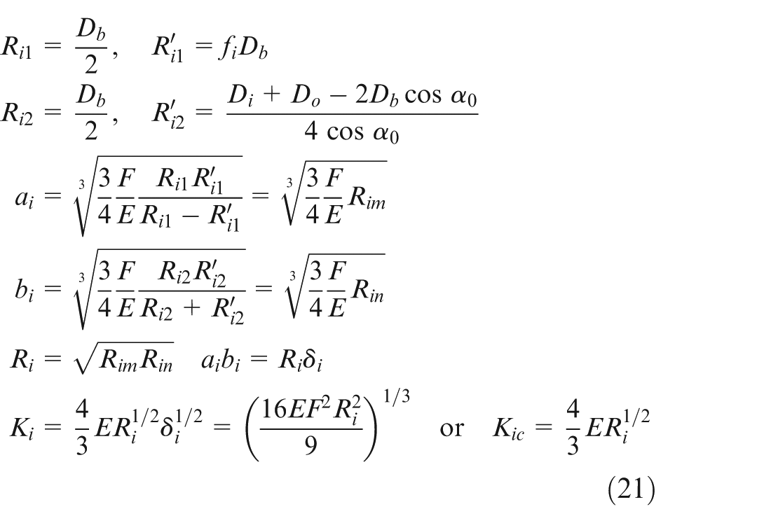
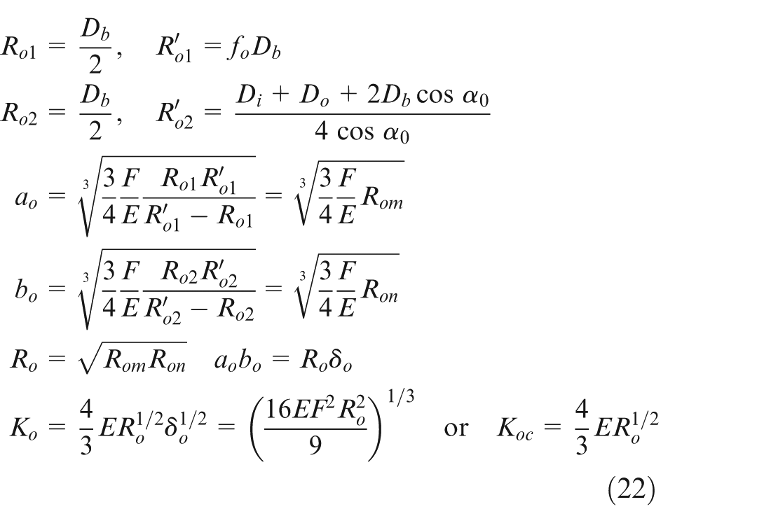
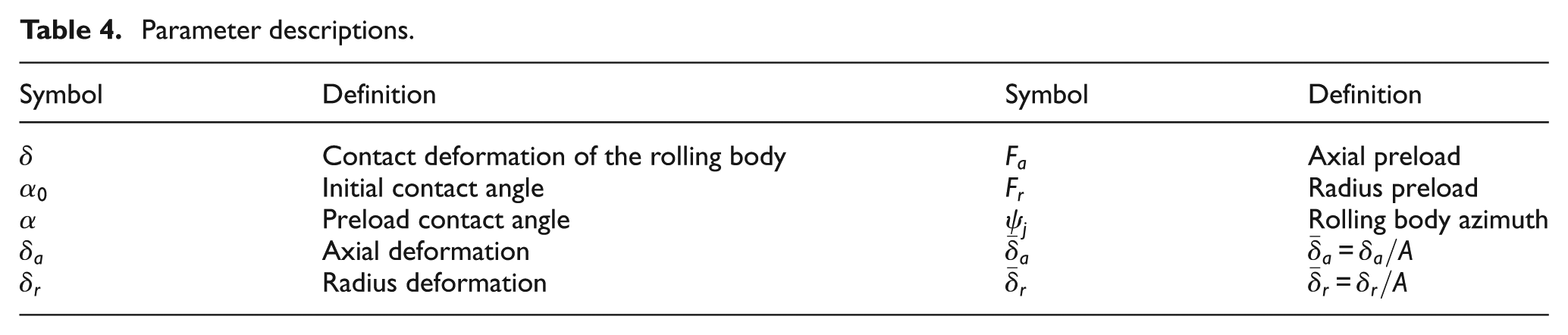
According to the Hertz contact theory, the contact stiffnesses of the inner and outer rings are calculated from equations (1)–(3) (i: inner ring and o: outer ring) (Table 4).

$$\begin{array}{cc}\multicolumn{1}{c}{R_{i1}}& =\frac{D_b}{2},R{\prime }_{i1}=f_i{D}_b\hfill \\ \multicolumn{1}{c}{R_{i2}}& =\frac{D_b}{2},R{\prime }_{i2}=\frac{D_i+D_o-2D_b\cos {\alpha }_0}{4\cos {\alpha }_0}\hfill \\ \multicolumn{1}{c}{a_i}& =\sqrt[3]{\frac{3}{4}\frac{F}{E}\frac{R_{i1}R{\prime }_{i1}}{R_{i1}-R{\prime }_{i1}}}=\sqrt[3]{\frac{3}{4}\frac{F}{E}{R}_{\mathrm{im}}}\hfill \\ \multicolumn{1}{c}{b_i}& =\sqrt[3]{\frac{3}{4}\frac{F}{E}\frac{R_{i2}R{\prime }_{i2}}{R_{i2}+R{\prime }_{i2}}}=\sqrt[3]{\frac{3}{4}\frac{F}{E}{R}_{\mathrm{in}}}\hfill \\ \multicolumn{1}{c}{R_i}& =\sqrt{R_{\mathrm{im}}{R}_{\mathrm{in}}}{a}_i{b}_i=R_i{\delta }_i\hfill \\ \multicolumn{1}{c}{K_i}& =\frac{4}{3}{\mathrm{ER}}_i^{1/2}{\delta }_i^{1/2}={\left(\frac{16{\mathrm{EF}}^2{R}_i^2}{9}\right)}^{1/3}\mathrm{or}{K}_{\mathrm{ic}}=\frac{4}{3}{\mathrm{ER}}_i^{1/2}\hfill \end{array}$$

(21)

$$\begin{array}{cc}\multicolumn{1}{c}{R_{o1}}& =\frac{D_b}{2},R{\prime }_{o1}=f_o{D}_b\hfill \\ \multicolumn{1}{c}{R_{o2}}& =\frac{D_b}{2},R{\prime }_{o2}=\frac{D_i+D_o+2D_b\cos {\alpha }_0}{4\cos {\alpha }_0}\hfill \\ \multicolumn{1}{c}{a_o}& =\sqrt[3]{\frac{3}{4}\frac{F}{E}\frac{R_{o1}R{\prime }_{o1}}{R{\prime }_{o1}-R_{o1}}}=\sqrt[3]{\frac{3}{4}\frac{F}{E}{R}_{\mathrm{om}}}\hfill \\ \multicolumn{1}{c}{b_o}& =\sqrt[3]{\frac{3}{4}\frac{F}{E}\frac{R_{o2}R{\prime }_{o2}}{R{\prime }_{o2}-R_{o2}}}=\sqrt[3]{\frac{3}{4}\frac{F}{E}{R}_{\mathrm{on}}}\hfill \\ \multicolumn{1}{c}{R_o}& =\sqrt{R_{\mathrm{om}}{R}_{\mathrm{on}}}{a}_o{b}_o=R_o{\delta }_o\hfill \\ \multicolumn{1}{c}{K_o}& =\frac{4}{3}{\mathrm{ER}}_o^{1/2}{\delta }_o^{1/2}={\left(\frac{16{\mathrm{EF}}^2{R}_o^2}{9}\right)}^{1/3}\mathrm{or}{K}_{\mathrm{oc}}=\frac{4}{3}{\mathrm{ER}}_o^{1/2}\hfill \end{array}$$

(22)

Table 4.

Parameter descriptions.

Symbol	Definition	Symbol	Definition
$\delta$	Contact deformation of the rolling body	$F_a$	Axial preload
${\alpha }_0$	Initial contact angle	$F_r$	Radius preload
$\alpha$	Preload contact angle	${\psi }_j$	Rolling body azimuth
${\delta }_a$	Axial deformation	${\overline{\delta }}_a$	${\overline{\delta }}_a={\delta }_a/A$
${\delta }_r$	Radius deformation	${\overline{\delta }}_r$	${\overline{\delta }}_r={\delta }_r/A$

Integrated contact stiffness

$$k=\frac{1}{1/K_i+1/K_o}\mathrm{or}{k}_c={\left(\frac{1}{{(1/K_{\mathrm{ic}})}^{2/3}+{(1/K_{\mathrm{oc}})}^{2/3}}\right)}^{3/2}$$

(23)

Axial and radial stiffnesses of the bearing

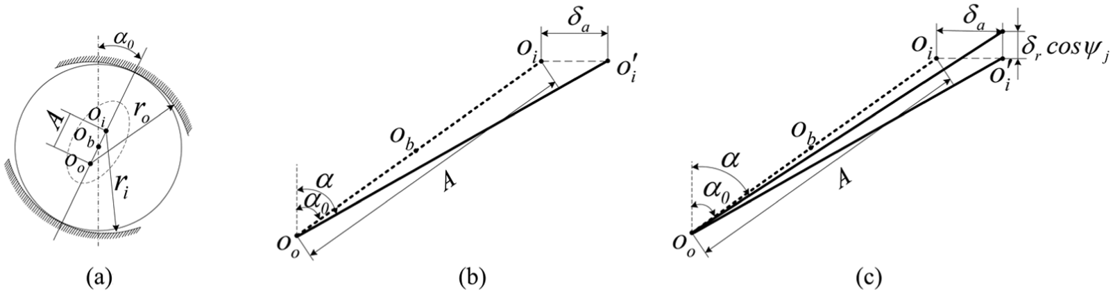
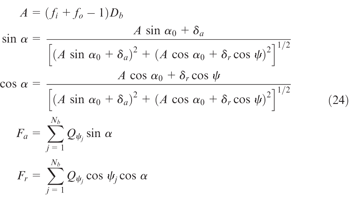
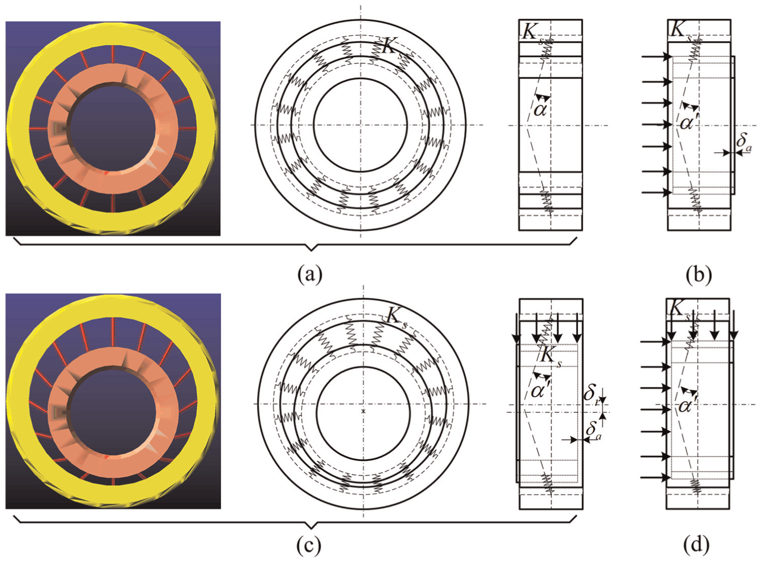
Figure 7 shows specific aspects of the contact geometry for a rolling body and those changes in its position relative to the inner and outer rings for different states of the system under study.

Figure 7.

Geometry of the rolling body positions: (a) relationship between rolling and inner and outer ring, (b) low speed and light load (axis preloading), and (c) low speed and heavy load (axis and radial preloading).

Geometrical and physical relationships

$$\begin{array}{cc}\multicolumn{1}{c}{A}& =(f_i+f_o-1)D_b\hfill \\ \multicolumn{1}{c}{\sin \alpha }& =\frac{A\sin {\alpha }_0+{\delta }_a}{{[{(A\sin {\alpha }_0+{\delta }_a)}^2+{(A\cos {\alpha }_0+{\delta }_r\cos \psi )}^2]}^{1/2}}\hfill \\ \multicolumn{1}{c}{\cos \alpha }& =\frac{A\cos {\alpha }_0+{\delta }_r\cos \psi }{{[{(A\sin {\alpha }_0+{\delta }_a)}^2+{(A\cos {\alpha }_0+{\delta }_r\cos \psi )}^2]}^{1/2}}\hfill \\ \multicolumn{1}{c}{F_a}& ={\displaystyle \sum _{j=1}^{N_b}}{Q}_{{\psi }_j}\sin \alpha \hfill \\ \multicolumn{1}{c}{F_r}& ={\displaystyle \sum _{j=1}^{N_b}}{Q}_{{\psi }_j}\cos {\psi }_j\cos \alpha \hfill \end{array}$$

(24)

Under low speed and light load

$$\begin{array}{cc}\multicolumn{1}{c}{}& \delta -A[{(1+{\overline{\delta }}_a^2+2{\overline{\delta }}_a\sin \left({\alpha }_0\right))}^{1/2}-1]=0\hfill \\ \multicolumn{1}{c}{}& \sin \left(\alpha \right){(1+{\overline{\delta }}_a^2+2{\overline{\delta }}_a\sin \left({\alpha }_0\right))}^{1/2}-(\sin \left({\alpha }_0\right)+{\overline{\delta }}_a)=0\hfill \\ \multicolumn{1}{c}{}& F_a/N_b-k_c{\delta }^{3/2}\sin (\alpha )=0\hfill \end{array}$$

(25)

Under low speed and heavy load

$$\begin{array}{cc}\multicolumn{1}{c}{}& \delta -A\{{[{(\sin \left({\alpha }_0\right)+{\overline{\delta }}_a)}^2+{(\cos \left({\alpha }_0\right)+{\overline{\delta }}_r\cos \left(\psi \right))}^2]}^{1/2}-1\}=0\hfill \\ \multicolumn{1}{c}{}& \{\begin{array}{c}\hfill \sin \left(\alpha \right){[{(\sin \left({\alpha }_0\right)+{\overline{\delta }}_a)}^2+{(\cos \left({\alpha }_0\right)+{\overline{\delta }}_r\cos \left({\psi }_j\right))}^2]}^{1/2}-(\sin \left({\alpha }_0\right)+{\overline{\delta }}_a)=0\hfill \\ \multicolumn{1}{c}{\cos \left(\alpha \right){[{(\sin \left({\alpha }_0\right)+{\overline{\delta }}_a)}^2+{(\cos \left({\alpha }_0\right)+{\overline{\delta }}_r\cos \left({\psi }_j\right))}^2]}^{1/2}-(\cos \left({\alpha }_0\right)+{\overline{\delta }}_r\cos \left({\psi }_j\right))=0}\end{array}\hfill \\ \multicolumn{1}{c}{}& F_a/N_b-k_c{\delta }^{3/2}\sin \left(\alpha \right)=0\hfill \\ \multicolumn{1}{c}{}& F_r-{\displaystyle \sum _{j=1}^{N_b}}\left(k_c{\delta }^{3/2}\cos \left(\alpha \right)\right)\cos \left({\psi }_j\right)=0\hfill \end{array}(26)$$

(26)

We solve equation (26)

$$F_{\mathrm{a}}-k_c{A}^{3/2}{\displaystyle \sum _{j=1}^{N_b}}\left(\begin{array}{c}\hfill {\{{[{(\sin \left({\alpha }_0\right)+{\overline{\delta }}_a)}^2+{(\cos \left({\alpha }_0\right)+{\overline{\delta }}_r\cos \left({\psi }_j\right))}^2]}^{1/2}-1\}}^{3/2}·\hfill \\ \multicolumn{1}{c}{\frac{\sin \left({\alpha }_0\right)+{\overline{\delta }}_a}{{[{(\sin \left({\alpha }_0\right)+{\overline{\delta }}_a)}^2+{(\cos \left({\alpha }_0\right)+{\overline{\delta }}_r\cos \left({\psi }_j\right))}^2]}^{1/2}}}\end{array}\right)=0(27)$$

(27)

$$F_r-k_c{A}^{3/2}{\displaystyle \sum _{j=1}^{N_b}}\left(\begin{array}{c}\hfill {\{{[{(\sin \left({\alpha }_0\right)+{\overline{\delta }}_a)}^2+{(\cos \left({\alpha }_0\right)+{\overline{\delta }}_r\cos \left({\psi }_j\right))}^2]}^{1/2}-1\}}^{3/2}·\hfill \\ \multicolumn{1}{c}{\frac{\cos \left({\alpha }_0\right)+{\overline{\delta }}_r\cos \left({\psi }_j\right)}{{[{(\sin \left({\alpha }_0\right)+{\overline{\delta }}_a)}^2+{(\cos \left({\alpha }_0\right)+{\overline{\delta }}_r\cos \left({\psi }_j\right))}^2]}^{1/2}}\cos \left({\psi }_j\right)}\end{array}\right)=0(28)$$

(28)

Axial and radial stiffnesses

$$\begin{array}{c}\multicolumn{1}{c}{k_a=\frac{{\mathrm{dF}}_a}{d{\delta }_a}=\frac{\partial F_a}{\partial {\delta }_a}+\frac{\partial F_a}{\partial \sin \alpha }\frac{\partial \sin \alpha }{\partial {\delta }_a}}\\ \multicolumn{1}{c}{k_r=\frac{{\mathrm{dF}}_r}{d{\delta }_r}=\frac{\partial F_r}{\partial {\delta }_r}+\frac{\partial F_r}{\partial \sin \alpha }\frac{\partial \sin \alpha }{\partial {\delta }_r}}\end{array}$$

(29)

Suppose that

$$\begin{array}{cc}\multicolumn{1}{c}{x}& =\sin {\alpha }_0+{\overline{\delta }}_a\hfill \\ \multicolumn{1}{c}{y}& =\cos {\alpha }_0+{\overline{\delta }}_r\cos {\psi }_j\hfill \\ \multicolumn{1}{c}{z}& ={(x^2+y^2)}^{1/2}\hfill \end{array}$$

(30)

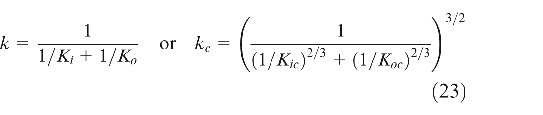
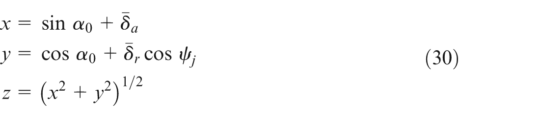
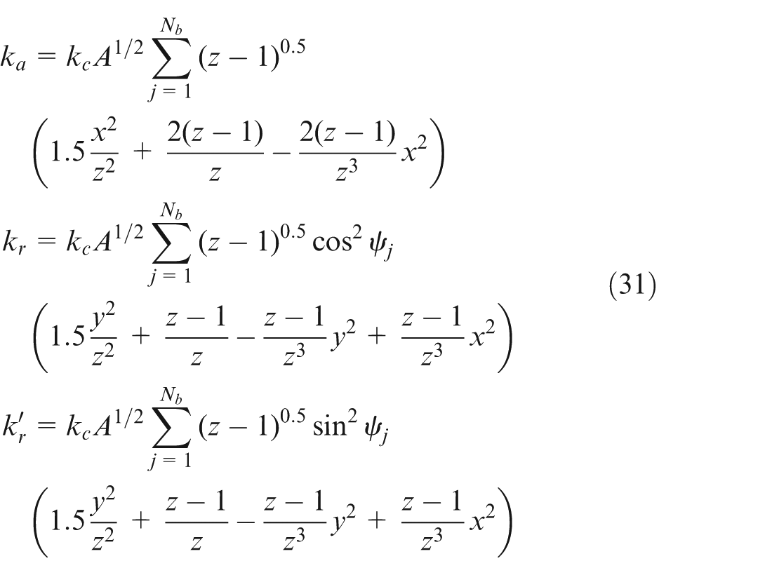
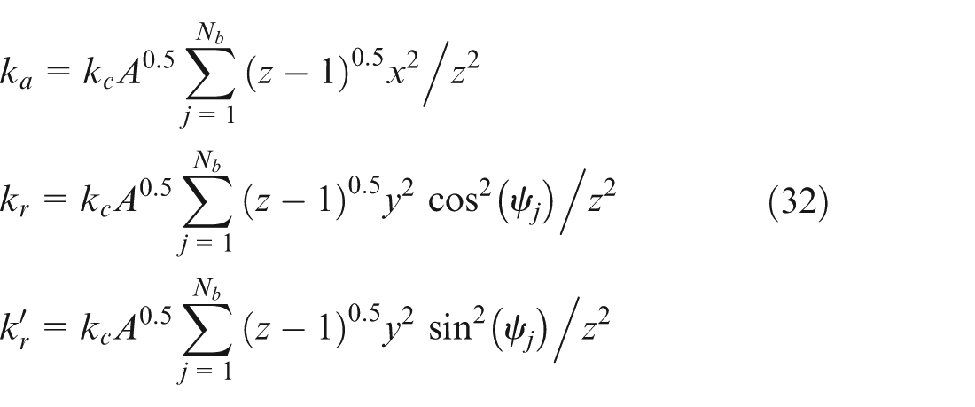
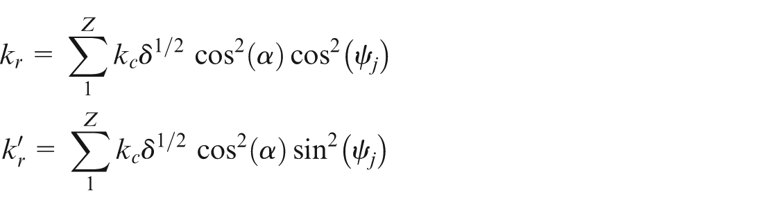
We then obtain axial stiffness $k_a$ , main radial stiffness $k_r$ which is the loaded direction, and second radial stiffness $k{\prime }_r$ which is perpendicular to the main radial stiffness

$$\begin{array}{cc}\multicolumn{1}{c}{k_a}& =k_c{A}^{1/2}{\displaystyle \sum _{j=1}^{N_b}}{(z-1)}^{0.5}\hfill \\ \multicolumn{1}{c}{}& (1.5\frac{x^2}{z^2}+\frac{2(z-1)}{z}-\frac{2(z-1)}{z^3}{x}^2)\hfill \\ \multicolumn{1}{c}{k_r}& =k_c{A}^{1/2}{\displaystyle \sum _{j=1}^{N_b}}{(z-1)}^{0.5}{\cos }^2{\psi }_j\hfill \\ \multicolumn{1}{c}{}& (1.5\frac{y^2}{z^2}+\frac{z-1}{z}-\frac{z-1}{z^3}{y}^2+\frac{z-1}{z^3}{x}^2)\hfill \\ \multicolumn{1}{c}{k{\prime }_r}& =k_c{A}^{1/2}{\displaystyle \sum _{j=1}^{N_b}}{(z-1)}^{0.5}{\sin }^2{\psi }_j\hfill \\ \multicolumn{1}{c}{}& (1.5\frac{y^2}{z^2}+\frac{z-1}{z}-\frac{z-1}{z^3}{y}^2+\frac{z-1}{z^3}{x}^2)\hfill \end{array}$$

(31)

Modelling and simulation of an angle-contact ball bearing

In the simulation process, a non-flexible and non-massive auxiliary outer bearing is added and revolves at the same angular velocity as the inner ring even though the outer ring is actually static. The rolling bodies are regarded as springs, whose stiffness equals the composition stiffness of the rolling body in contact with the inner and outer rings (equation (31)), and these springs connect the auxiliary bearing’s outer and inner rings. The spring’s stiffness and deflection angle $\alpha$ can be adjusted according to the axial and radial preload forces (Figure 8). In radial preload, there is a derived axial force due to the existence of the contact angle, so that the angle-contact ball bearing has a derived displacement of axial. In axial and radial preloading, the axial displacement should include the axial displacement produced by itself and the derived one from radial preload which could be ignored.

Figure 8.

Dynamic simulation modelling of an angle-contact ball bearing: (a) initial status, (b) axis preloading, (c) radial preloading, and (d) axis and radial preloading.

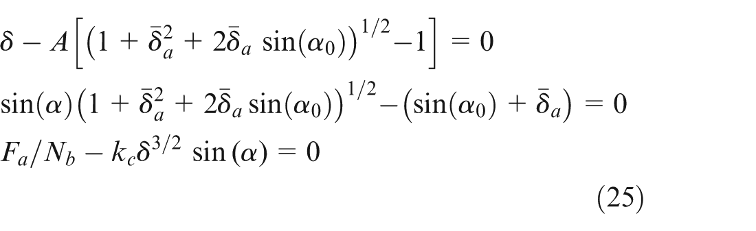
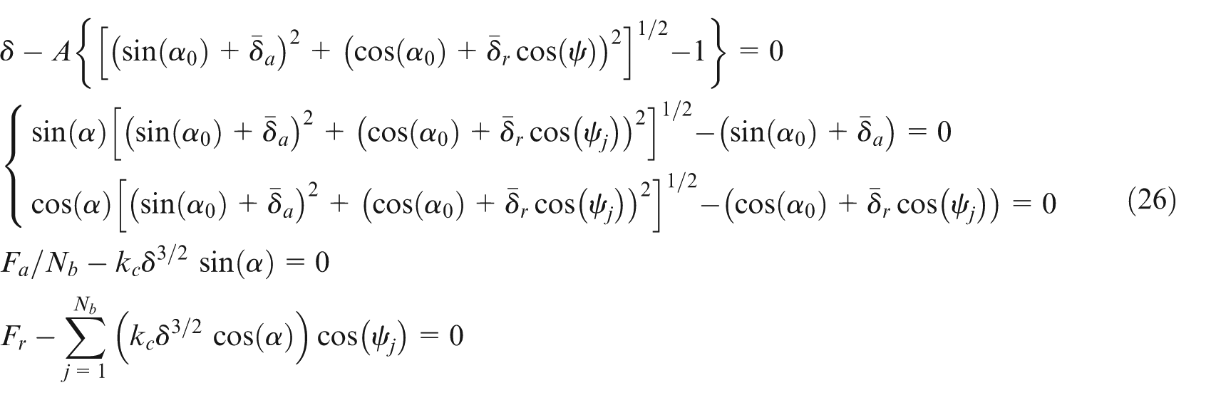
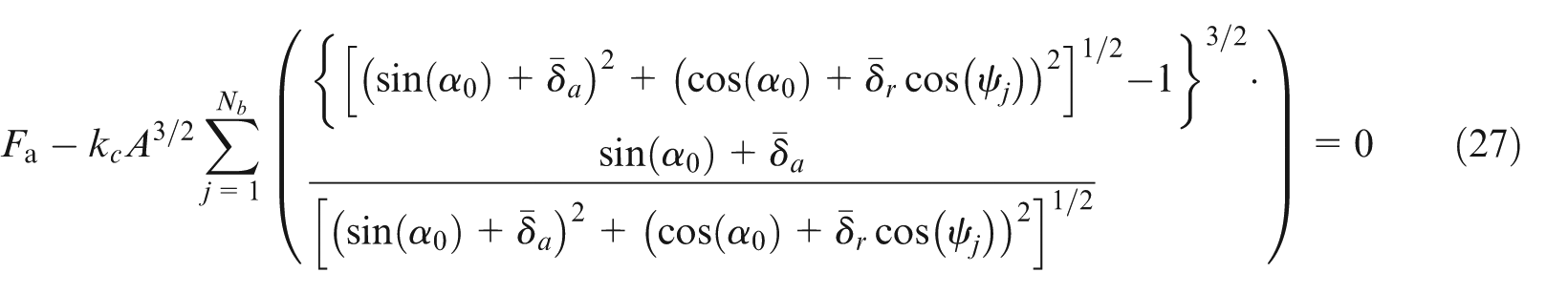
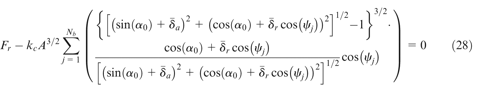
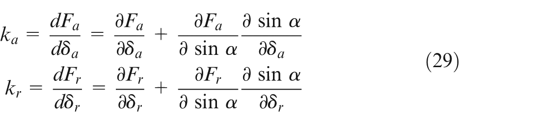
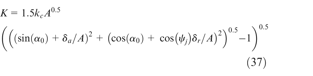
The dynamic simulation modelling actually facilitates the theoretical calculation formula of the axial and radial stiffnesses

$$\begin{array}{cc}\multicolumn{1}{c}{}& k_a=k_c{A}^{0.5}{\displaystyle \sum _{j=1}^{N_b}}{(z-1)}^{0.5}{x}^2/z^2\hfill \\ \multicolumn{1}{c}{}& k_r=k_c{A}^{0.5}{\displaystyle \sum _{j=1}^{N_b}}{(z-1)}^{0.5}{y}^2{\cos }^2\left({\psi }_j\right)/z^2\hfill \\ \multicolumn{1}{c}{}& k{\prime }_r=k_c{A}^{0.5}{\displaystyle \sum _{j=1}^{N_b}}{(z-1)}^{0.5}{y}^2{\sin }^2\left({\psi }_j\right)/z^2\hfill \end{array}$$

(32)

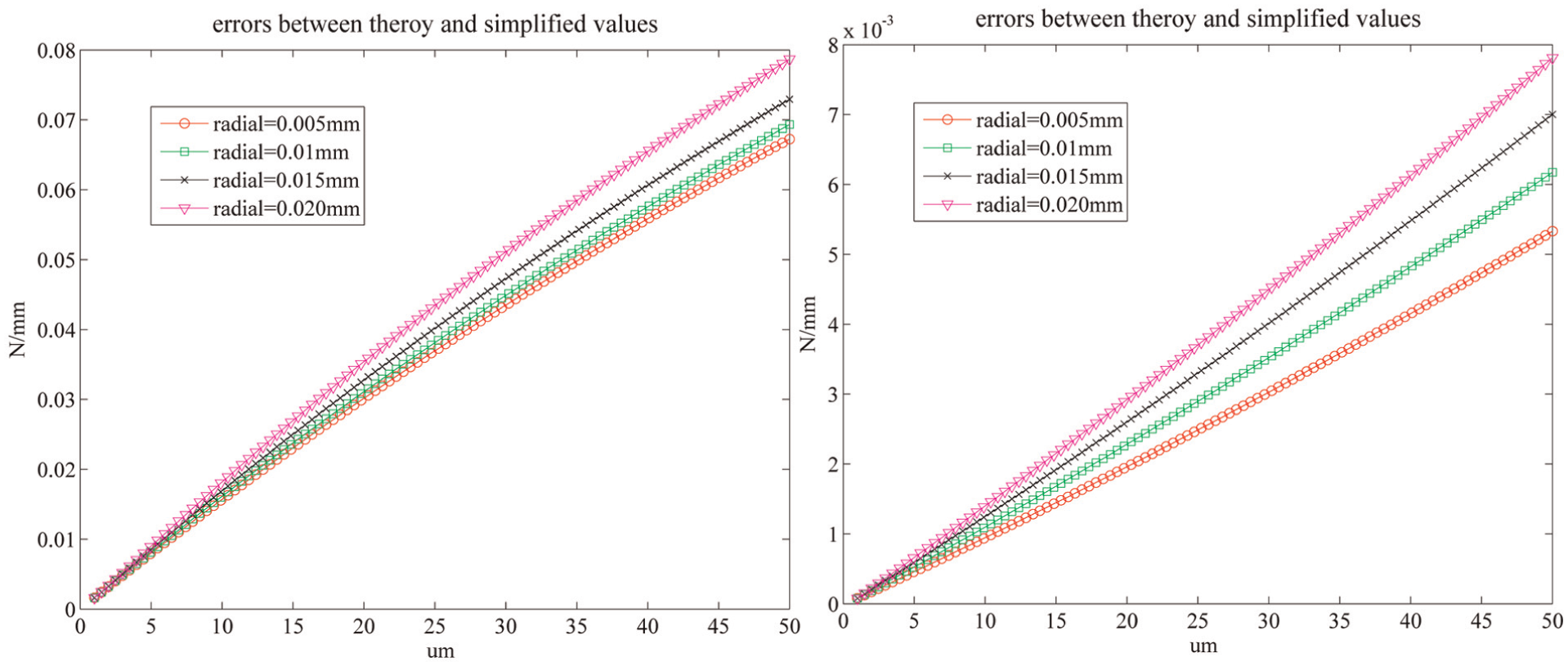
There are some differences between the theoretical calculation formula for the axial and radial stiffnesses (equation (31)) and the simplified calculation formula given above (equation (32)). Compare equation (31) with equation (32), when the first item is just reserved and the last items are ignored of equation (31), equation (32) can be obtained which is just less a scaling factor $\xi =1.5$ called correction coefficient derived from the index 3/2 of the $k-\delta$ relation. The simulation calculation equation (33) is

$$\begin{array}{cc}\multicolumn{1}{c}{k_a}& =\xi k_c{A}^{0.5}{\displaystyle \sum _{j=1}^{N_b}}{(z-1)}^{0.5}{x}^2/z^2=1.5{\displaystyle \sum _{j=1}^{N_b}}{\mathrm{kx}}^2{z}^2\hfill \\ \multicolumn{1}{c}{k_r}& =\xi k_c{A}^{0.5}{\displaystyle \sum _{j=1}^{N_b}}{(z-1)}^{0.5}{y}^2{\cos }^2\left({\psi }_j\right)/z^2\hfill \\ \multicolumn{1}{c}{}& =1.5{\displaystyle \sum _{j=1}^{N_b}}{\mathrm{ky}}^2\cos \left({\psi }_j\right)/z^2\hfill \\ \multicolumn{1}{c}{k{\prime }_r}& =\xi k_c{A}^{0.5}{\displaystyle \sum _{j=1}^{N_b}}{(z-1)}^{0.5}{y}^2{\sin }^2\left({\psi }_j\right)/z^2\hfill \\ \multicolumn{1}{c}{}& =1.5{\displaystyle \sum _{j=1}^{N_b}}{\mathrm{ky}}^2\sin \left({\psi }_j\right)/z^2\hfill & \hfill \end{array}$$

(33)

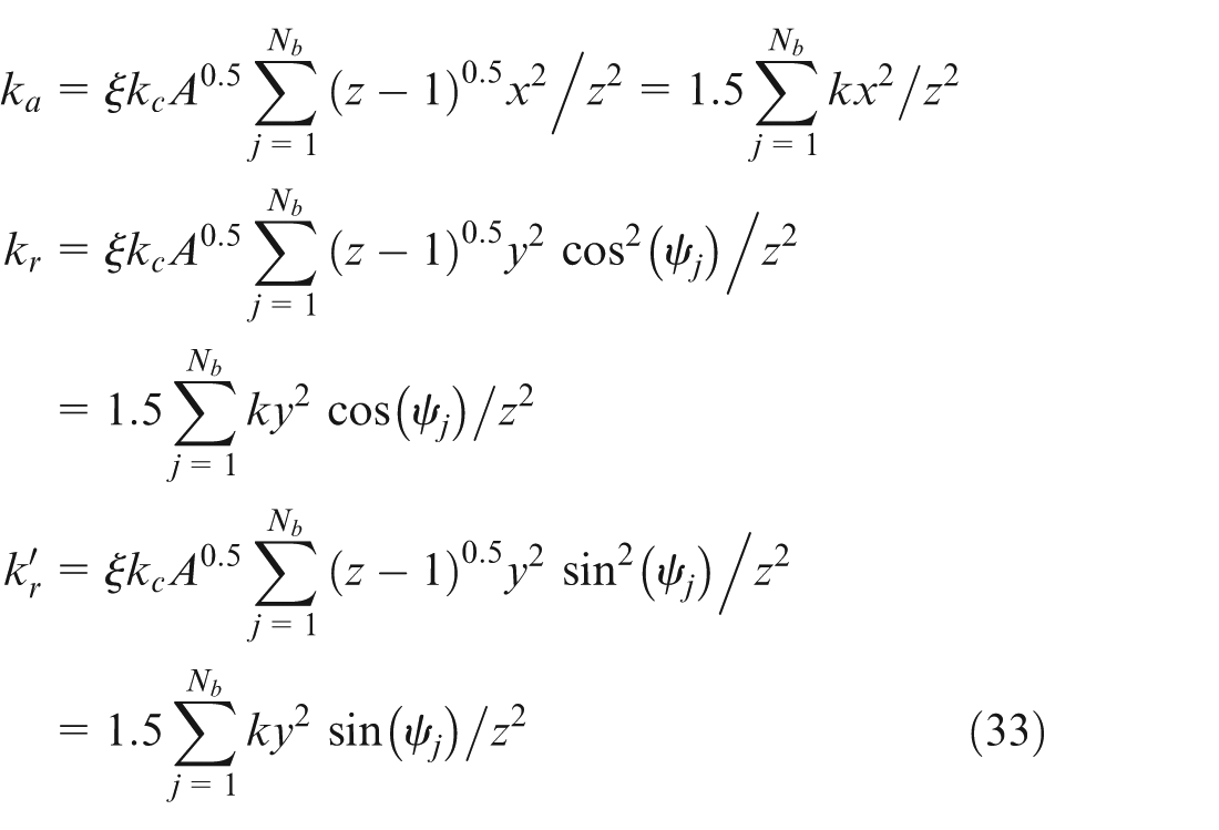
Figure 9 compares the values determined by the theoretical (equation (31)) and reduced calculations (simulation calculation equation (33)) for a maximum axial and radial preload deformations of ${\delta }_a=0.05\mathrm{mm}$ and ${\delta }_r=0.01\mathrm{mm}$ , respectively. From Figure 10, the error between theory and reduced values of axial stiffness is just less than 8% and the error of the radial stiffness is even less than the axial one (0.8%). Thus, the complex theoretical calculation formula can be replaced with the simplified model.

Figure 9.

Comparison of the theoretical stiffness and simplified value.

Figure 10.

Errors between the theoretical stiffness and simplified value.

Joint dynamic model of an anti-backlash gear and angle-contact ball bearing

Application of the simplified Hertz theory in the transmission system

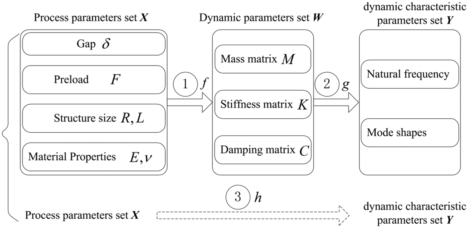
Mechanical products are assembled through different joints with surface contact, at which point the stiffness and damping characteristics of the surface have a strong influence on the overall dynamic performance. This article has attempted to establish a mapping relationship (1) $f(\delta ,F,R,L,E,\mu )$ using a simplification of the Hertz contact theory by exploring the theoretical formula relating the preload ( $F$ ), gap ( $\delta$ ), material properties ( $E,\mu$ , where $E$ is the equivalent elastic modulus and $\mu$ is the Poisson’s ratio), structure size (R, L, where $R$ is the equivalent radii and $L$ is the contact length), stiffness ( $K$ ), and damping ( $C$ ). The stiffness ( $K$ ) and damping ( $C$ ) were imported from commercial software (ADAMS) for dynamic simulation to implement a dynamic experiment, constituting a second mapping relationship (2) $g(M,K,C)$ between the kinetic parameters and dynamic characteristics, namely, the relationship among the stiffness ( $K$ ), the damping ( $C$ ), the natural frequency, and the vibration modes (namely, mechanical dynamic modelling, this is not the key point in article, therefore without list formulas). In fact, we ignored the damping in model. The reason is that it can simplify assembly model into a system without damping for convenience, and the influence of damping on the system natural frequency is limited. The combination of the dual mapping results ((1) and (2)) established a relationship (3) $h=f•g$ between alignment process parameters and the dynamic characteristics of the assembly (in Figure 11). We can change the process parameters to satisfy the dynamic demand of the assembly and make the alignment decision to optimize the process scheme and mining assembly data to predict the assembly performance.

Figure 11.

Dual mappings.

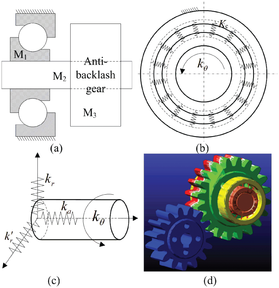
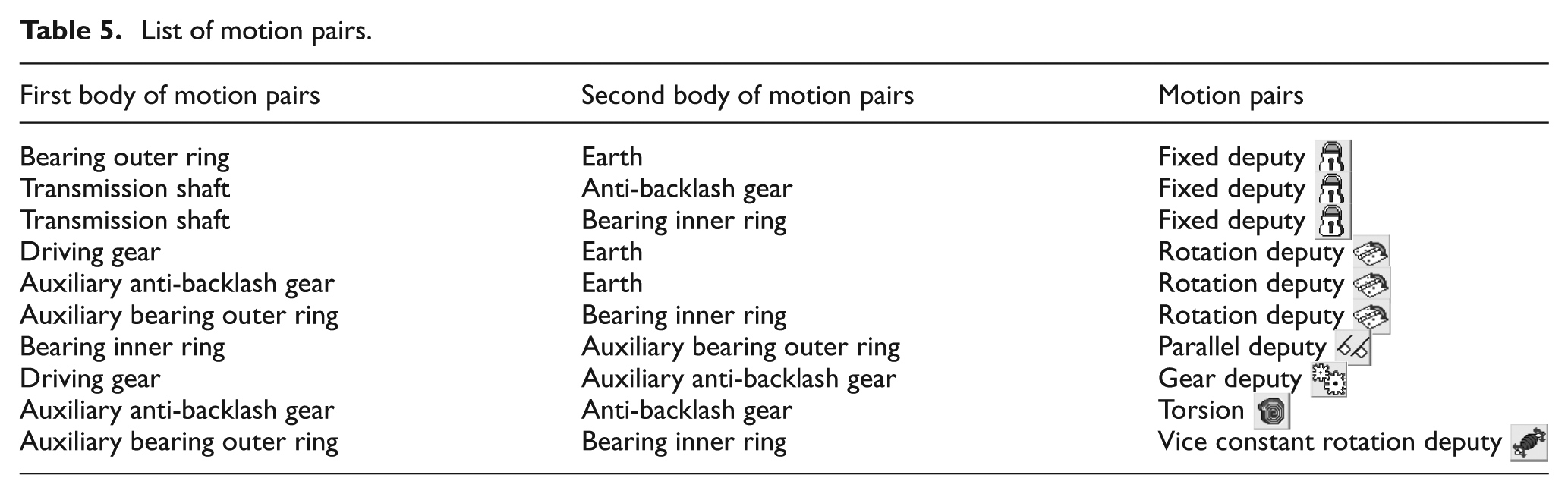
The transmission system model of an anti-backlash gear angle and angle-contact ball bearing can be simplified as shown in Figure 12(a). The outer ring of the bearing is a fixed and non-massive auxiliary ring is added with the same angular velocity as a motion unit $M=M_1+M_2+M_3$ , where the bearing inner ring is represented by $M_1$ , the transmission shaft is denoted by $M_2$ , and the anti-backlash gear is given as $M_3$ . Under the action of bearing contact stiffness and anti-backlash gear torsional stiffness, the motion unit presents 4 degrees of freedom: rotation around the shaft $k_{\theta }$ , axial translation along the axis of shaft $k_a$ , and two radial translations perpendicular to the axis of shaft $k_r,k{\prime }_r$ (Figure 12(c)). The rolling bodies are constrained by springs linking the auxiliary outer ring and motion unit which guarantee an adequate position of the rolling bodies. Using the dynamic simulation software program ADAMS, we can simulate the frequency response of the transmission system. As shown in Table 5, some motion pairs are added to ensure the system’s 4 degrees of freedom (as given in Figure 12(d)).

Figure 12.

Transmission system schematic diagram of an anti-backlash gear angle and angle-contact ball bearing.

Table 5.

List of motion pairs.

First body of motion pairs	Second body of motion pairs	Motion pairs
Bearing outer ring	Earth	Fixed deputy
Transmission shaft	Anti-backlash gear	Fixed deputy
Transmission shaft	Bearing inner ring	Fixed deputy
Driving gear	Earth	Rotation deputy
Auxiliary anti-backlash gear	Earth	Rotation deputy
Auxiliary bearing outer ring	Bearing inner ring	Rotation deputy
Bearing inner ring	Auxiliary bearing outer ring	Parallel deputy
Driving gear	Auxiliary anti-backlash gear	Gear deputy
Auxiliary anti-backlash gear	Anti-backlash gear	Torsion
Auxiliary bearing outer ring	Bearing inner ring	Vice constant rotation deputy

In Figure 12(c), the torsional stiffness $k_{\theta }$ is transformed by the contact stiffness of the anti-backlash gear

$$k_{\theta }=k_{\mathrm{st}}\times R_2^2$$

(34)

where $k_{s\mathrm{t}}$ represents the anti-backlash gear contact stiffness and $R_2$ is the base radius of the anti-backlash gear.

The axial stiffness $k_a$ represents the synthetic axial stiffness formed by all springs in parallel

$$k_a={\displaystyle \sum _{j=1}^{N_b}}{k}_c{\delta }^{1/2}{\sin }^2(\alpha )$$

(35)

The radial stiffness $k_r,k{\prime }_r$ represents the synthetic radial stiffness formed by all springs in parallel

$$\begin{array}{c}\multicolumn{1}{c}{k_r={\displaystyle \sum _1^Z}{k}_c{\delta }^{1/2}{\cos }^2\left(\alpha \right){\cos }^2\left({\psi }_j\right)}\\ \multicolumn{1}{c}{k{\prime }_r={\displaystyle \sum _1^Z}{k}_c{\delta }^{1/2}{\cos }^2\left(\alpha \right){\sin }^2\left({\psi }_j\right)}\end{array}$$

(36)

In ADAMS software, the rolling body is regarded as a spring, $\delta$ represents the deformation of the spring which is different along with the azimuth angle change and $1.5k_c{\delta }^{1/2}$ represents each spring’s stiffness. According to the axial displacement ${\delta }_a$ and maximum radial displacement ${\delta }_r$ , the spring stiffness vector is

$$\begin{array}{cc}\multicolumn{1}{c}{}& K=1.5k_c{A}^{0.5}\hfill \\ \multicolumn{1}{c}{}& {({({(\sin \left({\alpha }_0\right)+{\delta }_a/A)}^2+{(\cos \left({\alpha }_0\right)+\cos \left({\psi }_j\right){\delta }_r/A)}^2)}^{0.5}-1)}^{0.5}\hfill \end{array}$$

(37)

and $j=N_b$ . $K$ is derived from the spring compressing without elongating, so every element of it must be positive.

Simulation of the transmission system on axial preloading

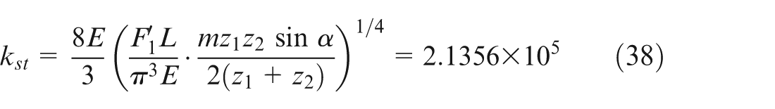
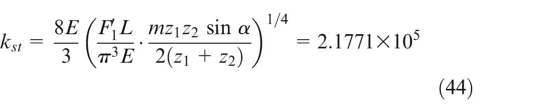
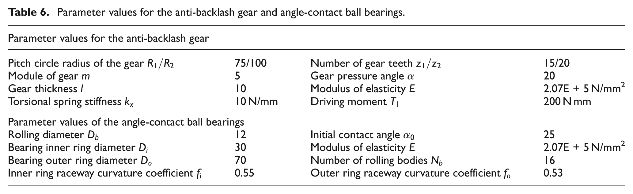
When the number of staggered teeth in the anti-backlash gear is 4 and the driving torque is T ₁=100Nm (the other parameters are listed in table 6), the gear meshing stiffness in theory is

$$k_{\mathrm{st}}=\frac{8E}{3}{(\frac{F{\prime }_{1}L}{{\pi }^{3}E}·\frac{{\mathrm{mz}}_1{z}_2\sin \alpha }{2(z_1+z_2)})}^{1/4}=2.1356\times {10}^5$$

(38)

Thus, the comprehensive torsional stiffness in theory is

$$k_{\theta }=k_{\mathrm{st}}\times R_2^2=2.1356\times {10}^9$$

(39)

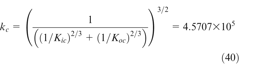
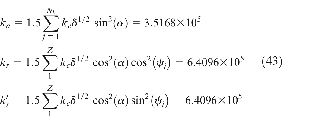
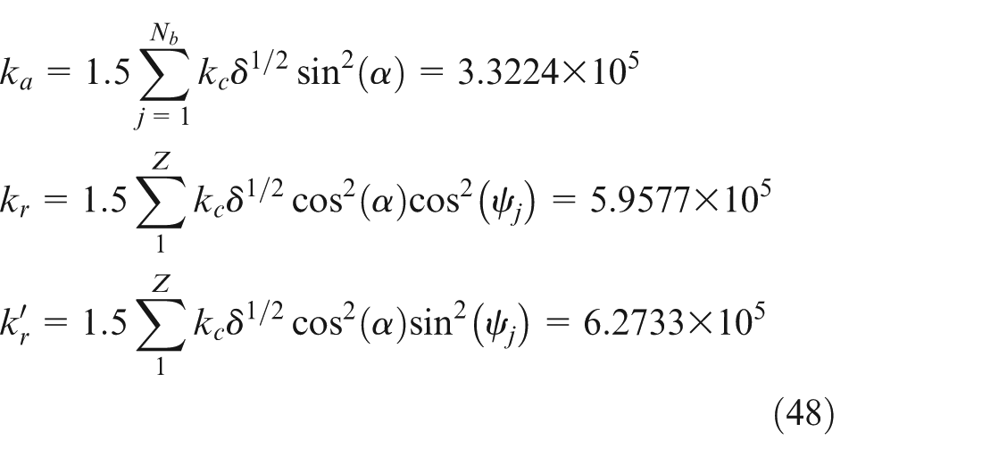
and the bearing integrated contact stiffness coefficient is

$$k_c={\left(\frac{1}{({(1/K_{\mathrm{ic}})}^{2/3}+{(1/K_{\mathrm{oc}})}^{2/3})}\right)}^{3/2}=4.5707\times {10}^5$$

(40)

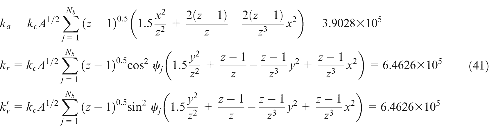
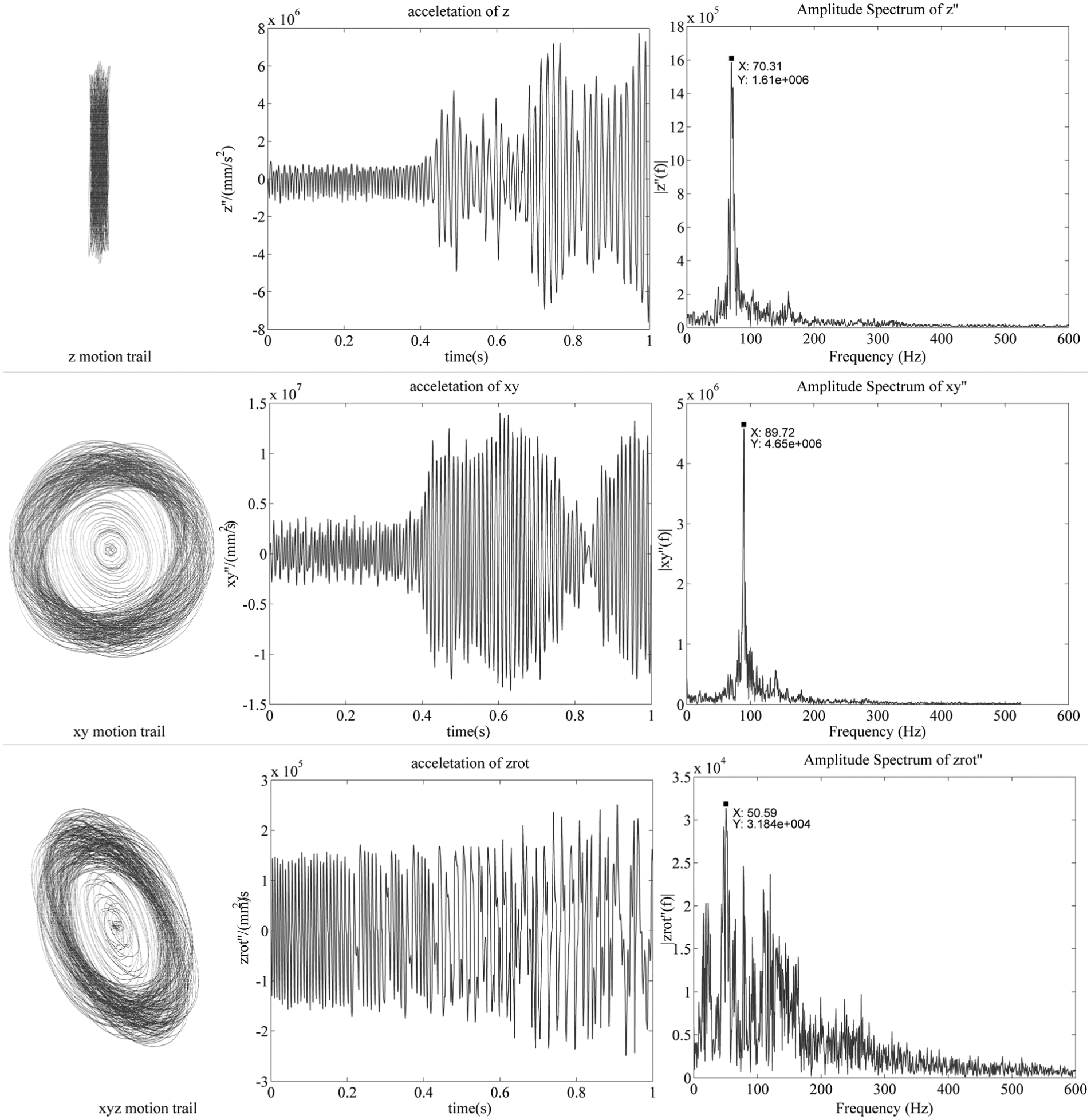
For an axial preload deformation of ${\delta }_a=0.05\mathrm{mm}$ and a radial preload maximum deformation of ${\delta }_r=0\mathrm{mm}$ (Figure 13), the bearing axial stiffness and radial stiffness in theory are

$$\begin{array}{cc}\multicolumn{1}{c}{}& k_a=k_c{A}^{1/2}{\displaystyle \sum _{j=1}^{N_b}}{(z-1)}^{0.5}(1.5\frac{x^2}{z^2}+\frac{2(z-1)}{z}-\frac{2(z-1)}{z^3}{x}^2)=3.9028\times {10}^5\hfill \\ \multicolumn{1}{c}{}& k_r=k_c{A}^{1/2}{\displaystyle \sum _{j=1}^{N_b}}{(z-1)}^{0.5}{\cos }^2{\psi }_j(1.5\frac{y^2}{z^2}+\frac{z-1}{z}-\frac{z-1}{z^3}{y}^2+\frac{z-1}{z^3}{x}^2)=6.4626\times {10}^5\hfill \\ \multicolumn{1}{c}{}& k{\prime }_r=k_c{A}^{1/2}{\displaystyle \sum _{j=1}^{N_b}}{(z-1)}^{0.5}{\sin }^2{\psi }_j(1.5\frac{y^2}{z^2}+\frac{z-1}{z}-\frac{z-1}{z^3}{y}^2+\frac{z-1}{z^3}{x}^2)=6.4626\times {10}^5\hfill \end{array}$$

(41)

Figure 13.

Dynamic performance of the transmission system (z′ = 4, δa = 0.05 mm, δr = 0).

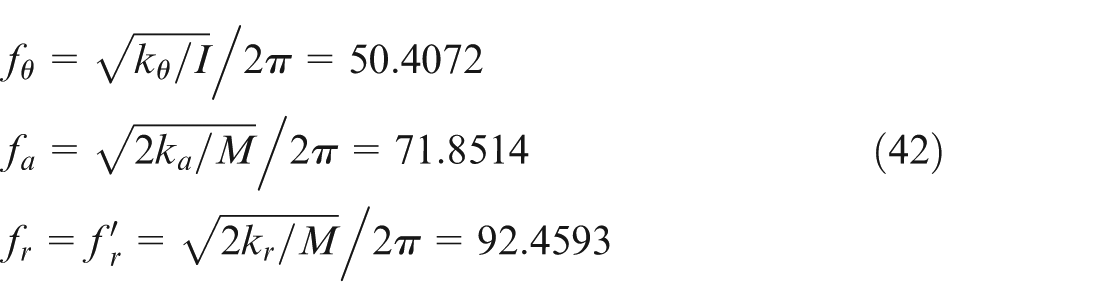
Therefore, the rotational, axial, and radial vibration frequencies of transmission system in theory are as follows ( $I=0.02129\mathrm{kg}{\mathrm{m}}^2,M=1.9149\mathrm{kg}$ , the moment of inertia and mass of the bearing inner ring, rotation shaft, and anti-backlash gear combined)

$$\begin{array}{cc}\multicolumn{1}{c}{}& f_{\theta }=\sqrt{k_{\theta }/I}/2\pi =50.4072\hfill \\ \multicolumn{1}{c}{}& f_a=\sqrt{2k_a/M}/2\pi =71.8514\hfill \\ \multicolumn{1}{c}{}& f_r=f{\prime }_r=\sqrt{2k_r/M}/2\pi =92.4593\hfill \end{array}$$

(42)

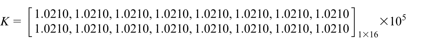
For simplified calculation model or simulation model for transmission system, the stiffness matrix is

$$K={\left[\begin{array}{c}\hfill 1.0210,1.0210,1.0210,1.0210,1.0210,1.0210,1.0210,1.0210\hfill \\ \multicolumn{1}{c}{1.0210,1.0210,1.0210,1.0210,1.0210,1.0210,1.0210,1.0210}\end{array}\right]}_{1\times 16}\times {10}^5$$

The stiffness of $N_b$ springs in simulation model is determined by $K$ . And the bearing axial stiffness and radial stiffness in the simulation model are

$$\begin{array}{cc}\multicolumn{1}{c}{}& k_a=1.5{\displaystyle \sum _{j=1}^{N_b}}{k}_c{\delta }^{1/2}{\sin }^2\left(\alpha \right)=3.5168\times {10}^5\hfill \\ \multicolumn{1}{c}{}& k_r=1.5{\displaystyle \sum _1^Z}{k}_c{\delta }^{1/2}{\cos }^2\left(\alpha \right){\cos }^2\left({\psi }_j\right)=6.4096\times {10}^5\hfill \\ \multicolumn{1}{c}{}& k{\prime }_r=1.5{\displaystyle \sum _1^Z}{k}_c{\delta }^{1/2}{\cos }^2\left(\alpha \right){\sin }^2\left({\psi }_j\right)=6.4096\times {10}^5\hfill \end{array}$$

(43)

Comparing equation (41) and (43), the synthetic stiffness on the theory and simulation is so close that the errors between them just fluctuate from 0.82% to 9.89%. From Figure 13, the similar the conclusion can be obtained: under an axial fixed-position preload only, the radial displacement presents a symmetrical distribution, and the radial resonant frequencies are equivalent and higher than the axial frequency. The dynamic results for the time and frequency domains display very good agreement.

Simulation of the transmission system on axial and radial preloading

When the number of staggered teeth in the anti-backlash gear is 5 and the driving torque is $T_1=100\mathrm{N\; m}$ and the other parameters are listed in Table 6, the gear meshing stiffness in theory is

$$k_{\mathrm{st}}=\frac{8E}{3}{(\frac{F{\prime }_{1}L}{{\pi }^{3}E}·\frac{{\mathrm{mz}}_1{z}_2\sin \alpha }{2(z_1+z_2)})}^{1/4}=2.1771\times {10}^5$$

(44)

Table 6.

Parameter values for the anti-backlash gear and angle-contact ball bearings.

Parameter values for the anti-backlash gear
Pitch circle radius of the gear $R_1/R_2$	75/100	Number of gear teeth $z_1/z_2$	15/20
Module of gear $m$	5	Gear pressure angle $\alpha$	20
Gear thickness $l$	10	Modulus of elasticity $E$	2.07E + 5 N/mm2
Torsional spring stiffness $k_x$	10 N/mm	Driving moment $T_1$	200 N mm
Parameter values of the angle-contact ball bearings
Rolling diameter $D_b$	12	Initial contact angle ${\alpha }_0$	25
Bearing inner ring diameter $D_i$	30	Modulus of elasticity $E$	2.07E + 5 N/mm2
Bearing outer ring diameter $D_o$	70	Number of rolling bodies $N_b$	16
Inner ring raceway curvature coefficient $f_i$	0.55	Outer ring raceway curvature coefficient $f_o$	0.53

Thus, the comprehensive torsional stiffness in theory is

$$k_{\theta }=k_{\mathrm{st}}\times R_2^2=2.1771\times {10}^9$$

(45)

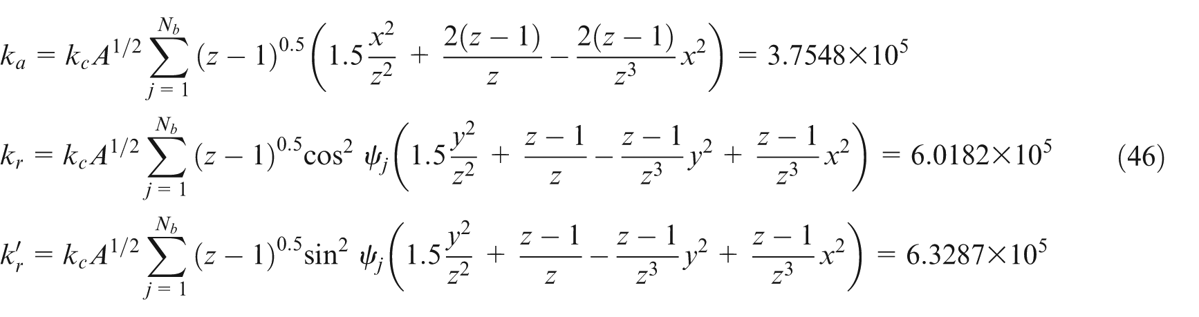
For an axial preload deformation of ${\delta }_a=0.05\mathrm{mm}$ and a radial preload maximum deformation of ${\delta }_r=0.02\mathrm{mm}$ (Figure 14), the bearing axial stiffness and radial stiffness in theory are

$$\begin{array}{cc}\multicolumn{1}{c}{}& k_a=k_c{A}^{1/2}{\displaystyle \sum _{j=1}^{N_b}}{(z-1)}^{0.5}(1.5\frac{x^2}{z^2}+\frac{2(z-1)}{z}-\frac{2(z-1)}{z^3}{x}^2)=3.7548\times {10}^5\hfill \\ \multicolumn{1}{c}{}& k_r=k_c{A}^{1/2}{\displaystyle \sum _{j=1}^{N_b}}{(z-1)}^{0.5}{\cos }^2{\psi }_j(1.5\frac{y^2}{z^2}+\frac{z-1}{z}-\frac{z-1}{z^3}{y}^2+\frac{z-1}{z^3}{x}^2)=6.0182\times {10}^5\hfill \\ \multicolumn{1}{c}{}& k{\prime }_r=k_c{A}^{1/2}{\displaystyle \sum _{j=1}^{N_b}}{(z-1)}^{0.5}{\sin }^2{\psi }_j(1.5\frac{y^2}{z^2}+\frac{z-1}{z}-\frac{z-1}{z^3}{y}^2+\frac{z-1}{z^3}{x}^2)=6.3287\times {10}^5\hfill \end{array}(46)$$

(46)

Figure 14.

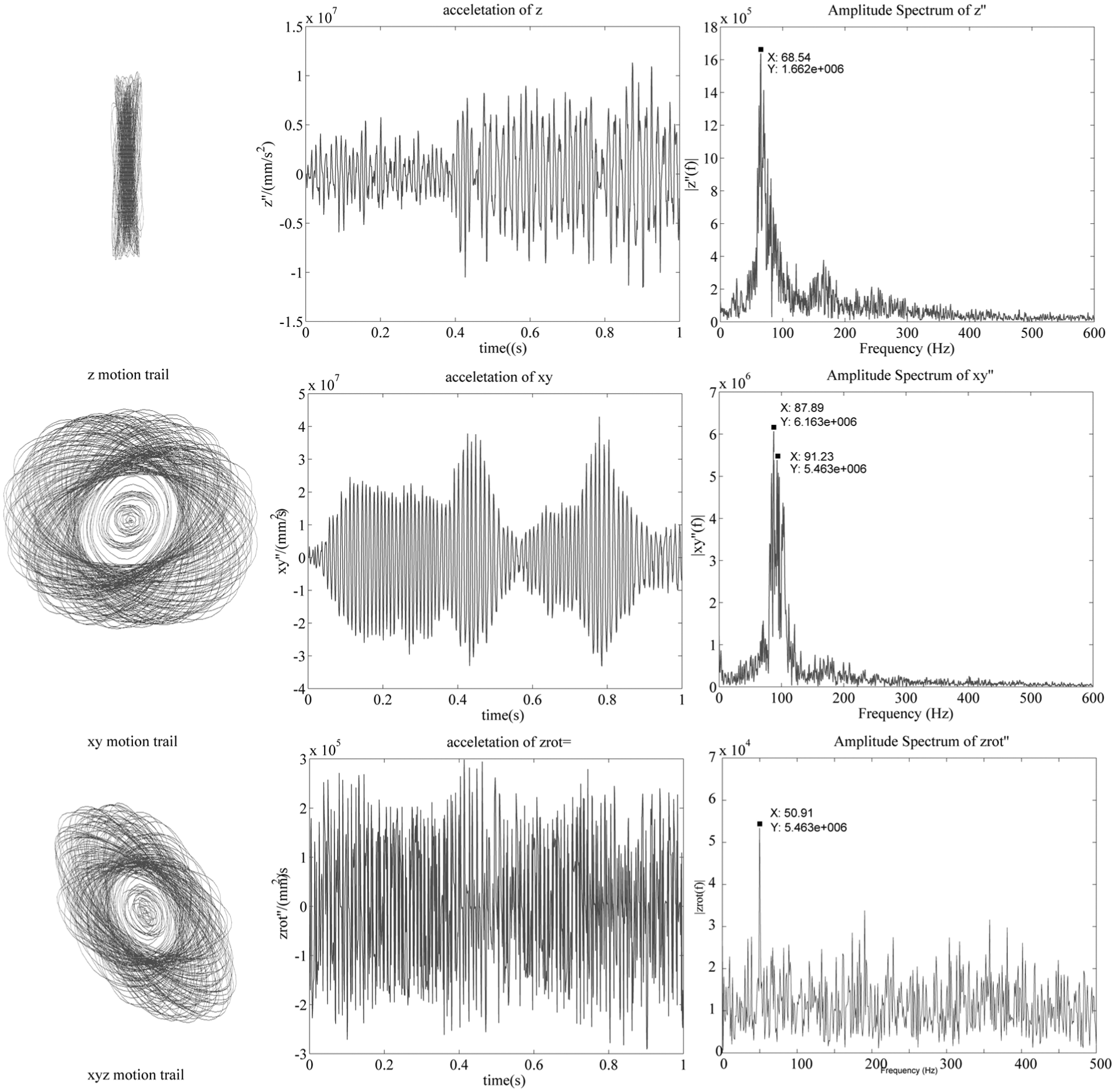
Dynamic performance of the transmission system (z′ = 5, δa = 0.05 mm, δr = 0.02 mm).

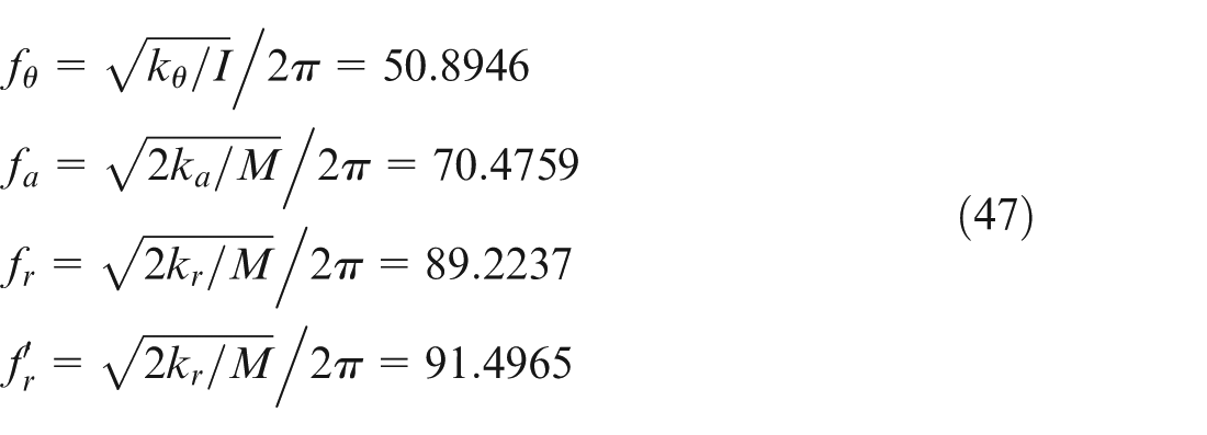
Therefore, the rotational, axial and radial vibration frequencies in the simulation model are as follows

$$\begin{array}{cc}\multicolumn{1}{c}{}& f_{\theta }=\sqrt{k_{\theta }/I}/2\pi =50.8946\hfill \\ \multicolumn{1}{c}{}& f_a=\sqrt{2k_a/M}/2\pi =70.4759\hfill \\ \multicolumn{1}{c}{}& f_r=\sqrt{2k_r/M}/2\pi =89.2237\hfill \\ \multicolumn{1}{c}{}& f{\prime }_r=\sqrt{2k_r/M}/2\pi =91.4965\hfill \end{array}$$

(47)

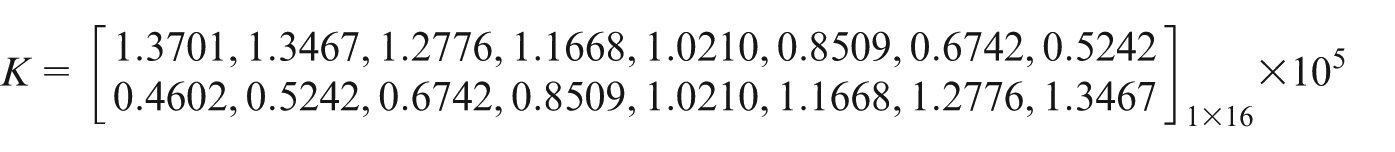
For simplified calculation model or simulation model for transmission system, the stiffness matrix is

$$K={\left[\begin{array}{c}\hfill 1.3701,1.3467,1.2776,1.1668,1.0210,0.8509,0.6742,0.5242\hfill \\ \multicolumn{1}{c}{0.4602,0.5242,0.6742,0.8509,1.0210,1.1668,1.2776,1.3467}\end{array}\right]}_{1\times 16}\times {10}^5$$

The stiffness of $N_b$ springs in simulation model is determined by $K$ . And the bearing axial stiffness and radial stiffness in the simulation model are

$$\begin{array}{cc}\multicolumn{1}{c}{}& k_a=1.5{\displaystyle \sum _{j=1}^{N_b}}{k}_c{\delta }^{1/2}{\sin }^2\left(\alpha \right)=3.3224\times {10}^5\hfill \\ \multicolumn{1}{c}{}& k_r=1.5{\displaystyle \sum _1^Z}{k}_c{\delta }^{1/2}{\cos }^2\left(\alpha \right){\cos }^2\left({\psi }_j\right)=5.9577\times {10}^5\hfill \\ \multicolumn{1}{c}{}& k{\prime }_r=1.5{\displaystyle \sum _1^Z}{k}_c{\delta }^{1/2}{\cos }^2\left(\alpha \right){\sin }^2\left({\psi }_j\right)=6.2733\times {10}^5\hfill \end{array}$$

(48)

Comparing equation (46) and (48), the synthetic stiffness on the theory and simulation is so close that the errors between them just fluctuate from 0.88% to 11.5289%. From Figure 14, the similar the conclusion can be obtained: under an axial and radial fixed-position preload, the radial displacement presents an asymmetrical flat distribution, and the radial resonant frequency in the fixed-preload direction is higher than that outside the preload direction, both of which are higher than the axial frequency.

According to the above analysis, in order to improve the rotational natural frequency of the transmission system, the driving torque or staggered teeth should be increased; in order to improve the axial and radial natural frequency of the transmission system, the axial preload deformation or radial preload deformation should be enhanced. But the preload could not increase infinitely; otherwise, the system could not motion because of the friction (although this aspect has not been involved in for this article).

Conclusion

The following conclusions are drawn:

1. The various mechanical joint surfaces and contact forms can be classified into some contact form of sphere or cylinder against a rigid flat plane. The Hertz theory focused on the stress and strain has been extended to study the stiffness between mechanical joint surfaces, and the complex formulas have been simplified to facilitate grasp and operation. Finally, the contact stiffness is come down to calculate the equivalent contact radius or contact area of contact surfaces, according to the geometries of the interacting bodies and their material properties.

2. The anti-backlash gear is simplified as a contact between two columns, and the gear meshing stiffness is reduced to torsional stiffness. By adding a non-massive rigid auxiliary gear, the torsional stiffness loaded between the auxiliary gear and anti-backlash gear can be simulated as the gear transmission, and the preload’s effect on the anti-backlash gear with respect to the rotation harmonic frequency can also be studied. Angle-contact ball bearings can also be simplified as springs connecting the inner and outer rings. The radial and axial stiffness represents the combined effect of these springs. By adding a non-massive rigid outer ring with the same revolution speed of the inner ring, the springs are constrained to be non-skewed, and thus, the support structure’s translation frequency can be simulated.

3. The contact stiffness determined by the simplified model is in good agreement with the theoretical value. Hence, we can replace the complex theoretical calculation formula with the simplified model.

4. The dynamic results for the time and frequency domains correspond well with one another. Furthermore, the presented simulation model can be used to predict dynamic performance, help the technicians to make alignment decisions and optimize the alignment scheme for the transmission in advance.