
Abstract
Fused deposition modelling is one of the additive manufacturing techniques in which part quality is often influenced by stair-step effects and internal meso-structures. Adaptive slicing employing slices of varying thicknesses was attempted as a means of overcoming some of these problems, but with limited success, while speed and time of printing often lead to further complications. On the other hand, curved layer deposition is proved to improve surface quality and part strength in specific cases. This research brings both flat and curved layer approaches together through specific algorithms developed and employed combining the two to process given parts. The mixed slicing method is applied successfully to three test cases, practically implemented on a test bed, and proved to be feasible and effective.
Introduction
Fused deposition modelling (FDL) is one of the additive manufacturing (AM) processes that gained considerable amount of popularity in the recent past. While the easy availability of different commercial solutions and increasing and cheaper material options are predominant reasons, the process also has inherent capabilities to produce parts of sufficient quality direct from computer-aided design (CAD) files. As with any AM technique, FDL typically allows reproduction of complex detail, which becomes increasingly important considering the suitability of the process especially for biomedical applications. 1 Typical shortcomings include stair-step effects resulting in poor surface quality and missing finer part details, depending on layer thicknesses used. While there are existing solutions to both these problems, the current research looks at combining two different techniques together to efficiently handle both surface and part quality problems together.
Adaptive slicing techniques were developed initially to overcome the problems due to stair-step effects and very fine geometrical details. The general approach through adaptive slicing is to divide the CAD model into critical and non-critical domains. Regions including intricate details or surfaces with steep slopes where stair-stepping effects could be more detrimental are critical and need to be filled with finer layers. Other non-critical regions are filled with either thicker layers or scaffold-like structures, targeting shorter build times. A number of different approaches are reported for adaptive slicing in the literature. Dolenc and Makela 2 first developed a basic adaptive slicing method to restrict the stair-step effect to a user-specified tolerance level. Sabourin et al. 3 followed a two-way approach: the first one considers regions with complex details as critical, while the second one considers external surfaces as critical and internal regions as non-critical. 4 Tyberg and Bohn 5 developed a local adaptive slicing model, based on identifying individual parts and individual part features to eliminate the use of thinner layers all through. Mani et al. 6 introduced a region-based adaptive slicing by considering the regions close to curved surfaces as critical regions. Pandey et al. 7 proposed a real-time edge profile adaptive slicing, which differs from Dolenc and Makela’s method and uses the roughness of the surface as the cusp height. While there are other approaches in similar lines,8,9 all these attempts mostly strive to reduce the intensity of the inherent shortcomings through adaptive slicing, but cannot altogether eliminate the problems. In order to eliminate the stair-case effects, Chakraborty et al. 10 proposed a curved layer fused deposition modelling (CLFDM) algorithm and tested on parametric surfaces. Singamneni et al. 11 further developed the curved layer slicing model using a vector–cross product algorithm and practically implemented the same while printing acrylonitrile butadiene styrene (ABS) test pieces. Experimental results based on three-point bending tests showed a marked improvement in the strength of thin shell parts printed by CLFDM, apart from eliminating stair-step effects.
Evidently, adaptive slicing involves dividing the part domain into different regions and using layers of varying thicknesses depending on the requirements in each zone. While reduced stair-step effects, better part strength and reduced printing time are all attributed to adaptive slicing, the analytical and experimental evaluations conducted by the authors prove the mechanics to be more complex and often leading to conflicting results. 12 The time to print a unit length of the polymer filament decides the rate of coalescence across adjacent filaments. Both time and speed of printing interact with each other and will influence the final part characteristics together with the filament size or the layer thickness. While apprehending the beneficial role of differential slicing, the proposal here is to choose between curved and flat layer slicing for different regions of the given solid. Deriving inspirations from the accurate external, fast internal slicing 4 and region-based adaptive slicing 6 algorithms, a new slicing process combining both curved and flat layer slicing is developed in this research. The basic approach is to slice the exterior with curved layers in order to capture finer details effectively as well as eliminate the stair-step effects while uniform flat layers are used in the interior. The first step of the proposed combined model involves development of an algorithm for dividing the CAD model into curved and flat layer regions. Appropriate curved and flat layer slicing schemes are implemented next in the respective zones, together with algorithms for integrating the deposition paths generated.
Subdividing a model based on the .stl format
To achieve combined curved and flat layer deposition, it is necessary to divide the domain into two distinct regions: the curved layer and the adaptive flat layer slicing regions. The .stl format file system, as the de facto data standard for AM, has been widely used for transferring the CAD model data into the AM processing area. It consists of a mesh of triangular facets representing the outside shell of the solid object, where each triangular facet shares the sides with adjacent elements and the vertices are ordered by the right-hand rule. It also lists the x, y and z coordinates of the three vertices of each surface triangle, with an index to describe the orientation of the surface normal. 13 Considering that slicing the .stl file is much easier compared to slicing models developed by other methods like B-rep and constructive solid geometry (CSG), all the algorithms developed as part of this research use data from the .stl file as the basis.
A simple slight-curved part as shown in Figure 1 is considered first to demonstrate the methods developed. The slicing process usually begins after the part orientation is selected, the first step being data acquisition from the .stl format file. For the current research, the top-surface data are critical, including the facets, vertices and normal directions. The .stl format file defines six specific faces: top and bottom, front and back, and left and right as shown in Figure 1, for the sample test piece considered. The areas are defined as follows.
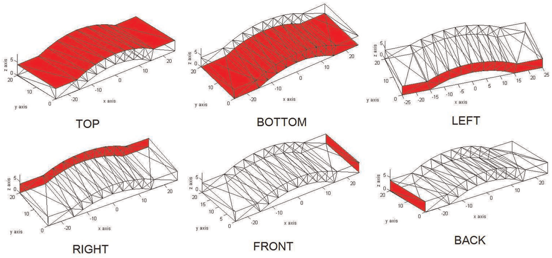
Surface definitions based on the .stl format file.
Top, bottom and side facets are defined by the angle between the normal vector and z-axis


Front, back, left and right facets are defined by the angle between the normal and x-axis following the counterclockwise direction


After identifying the probable top surface based on the information from the .stl file, a further refinement is usually necessary to differentiate between the top and side facets, based on minor variations in specific forms. The algorithm proposed by Dolenc and Makela 2 uses the cusp height to develop adaptive layers using the following equation

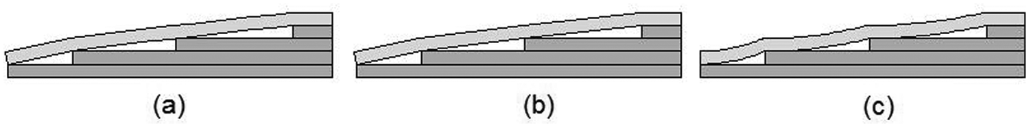
Based on equation (1), a user-defined cusp height is the local control parameter to differentiate between the top and side surfaces. Once the included angle is defined, the top original reference surface (surface to be offset) and the side surface (non-offsetting surface) can be differentiated. Subsequently, some further processing may often become necessary as it may not always be a single continuous surface as shown in Figure 2(a), but may be split into a number of segments as shown in Figure 2(b) and (c). The algorithms developed as part of this research cannot handle multiple surface sets simultaneously, as it gets quite complex while deciding the curved layer slicing strategies. As a result, further to identifying the top-surface facets, a facet grouping algorithm is used to identify the highest segment of the marked areas as the true top surface for initiating the curved layer slicing. This is done first identifying the highest point on the top surface and then processing the facets linked around this point. Once the facets immediately around the highest point are located, the search zone is expanded to find all connected facets. Figure 3 depicts this process with a sample part having a single continuous top surface.
The highest point was selected as the reference point.
If the vertex of a facet equals to the reference point, the facet is added to the top-surface group.
Other vertices of those facets are selected to be the new reference points.
Other facets are identified based on the new reference points and added to the top surface.
New referencing points are selected to replace the previous ones.
This procedure is repeated until no more facets could be gathered.
The top-surface facets are all grouped together.
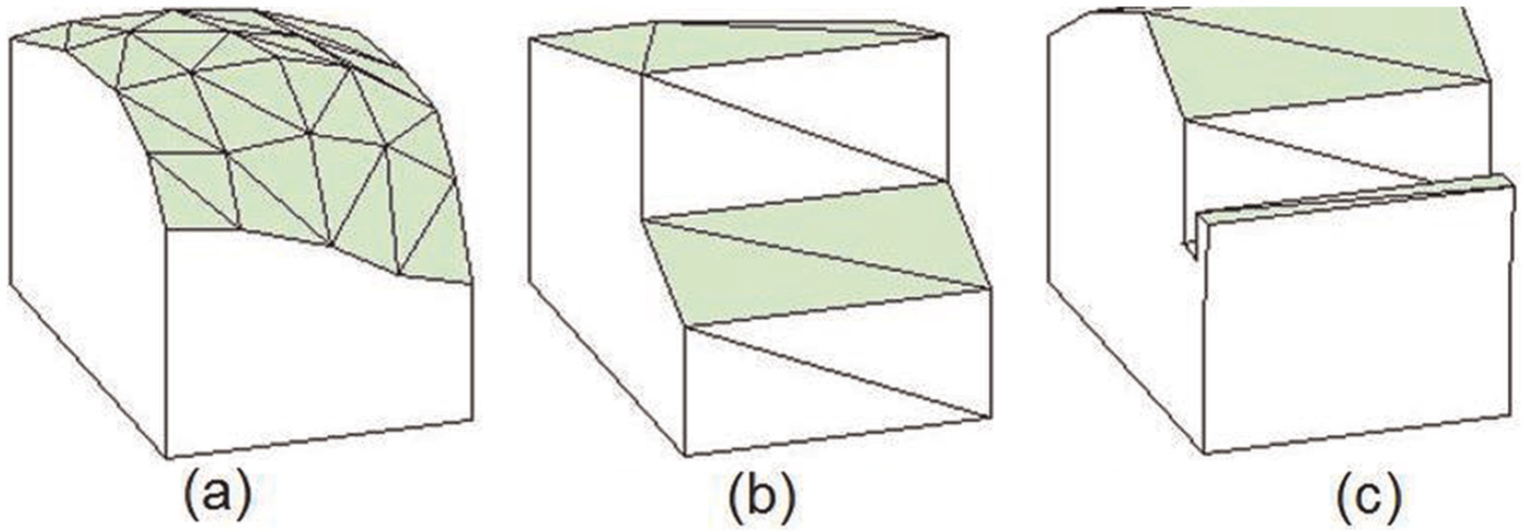
Continuity of top surface: (a) continuous facets, (b) non-continuous facets and (c) non-continuous facets.
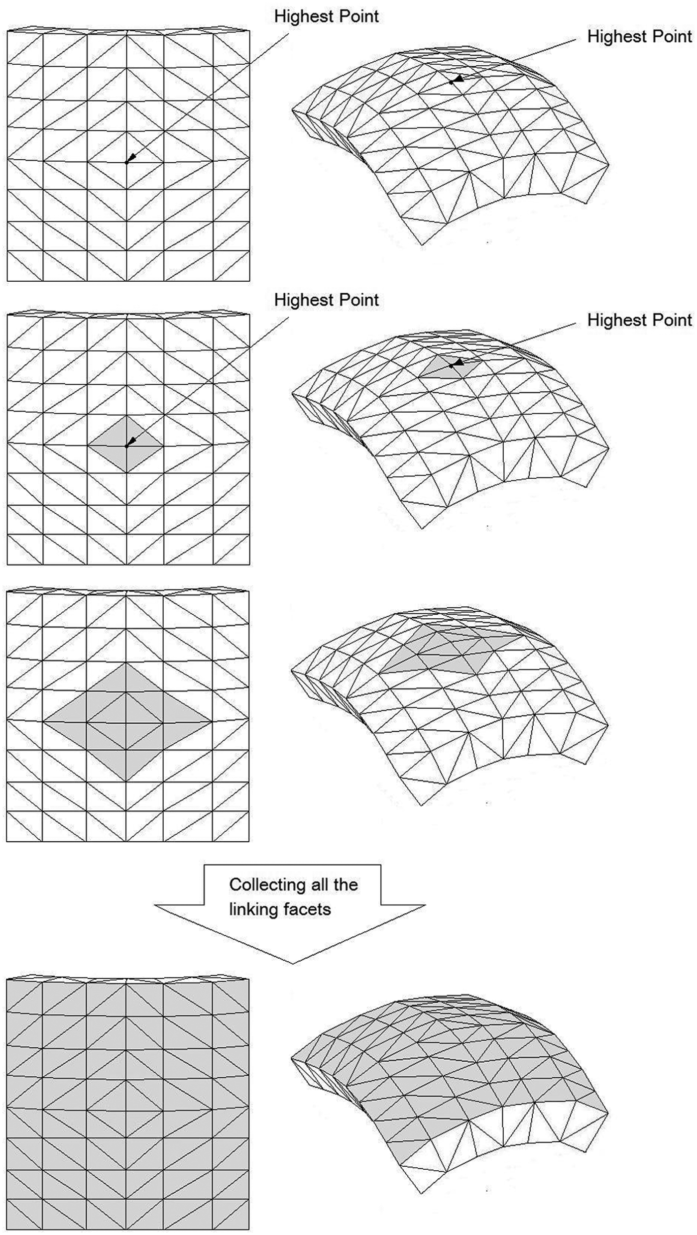
Facet grouping procedure.
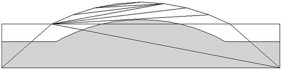
Once the top-surface data are gathered, the next step is to divide the domain into curved and flat layer regions. Considering the required quality of the top surface, the curved layer slicing takes precedence over the other and should take place using the point cloud data of the top surface. Flat layers takeover at some stage, and it is necessary to establish the boundary between the two regions. The criterion used to decide this boundary is based on observations on the pattern of flat layers deposited on supporting scaffold structures. Figure 4 depicts flat layer filaments deposited on vertical scaffold structures of varying span. As evident from Figure 4(a), the filament normally sags under its own weight and the associated plasticity. This effect can be eliminated by printing multiple layers on the same support structure as shown in Figure 4(b) or by reducing the span length as shown in Figure 4(c). Now, comparing the curved layers deposited over flat layers as shown in Figure 5, with the flat layer cases of Figure 4, it may be observed that the detrimental effects due to filament sagging can be controlled by using either successively stacked layers as shown in Figure 4(b) or by reducing the span length between successive legs of the support structure as shown in Figure 4(c). When curved layers are deposited over flat layers, the boundary condition between the two regions will be shown in Figure 5(a). Ideally, the curved layer is laid on top of the flat layers and represents the actual shape of the part, mostly using curves or splines. In the deposition system, all the curves or splines are converted to straight line segments, as shown in Figure 5(b). In the actual deposition, the curved layer is a composite of strands. These semi-solid strands are still soft when they are just extruded out of the nozzle. Therefore, they do not exactly represent the shape of the surface; instead, they will bend due to gravity, as shown in Figure 5(c). Similar to the cusp height, a chordal height evaluation is used here to identify the boundary between curved and flat layer regions.
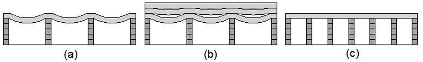
Issues with flat layer deposition and solutions: (a) bending phenomenon during deposition, (b) Multi-layer solution, and (c) Reduced gaps solution.
Boundary between curved and flat layer regions: (a) ideal case, (b) based on tool paths and (c) the true case.
Chordal error was first mentioned by Agarwala et al. 14 describing the defects arising from piecewise linear segments used to represent a curved surface. The chordal height is used here as the criterion to determine the magnitude of the region to be filled with curved layers in order to eliminate the stair-case effects based on the maximum allowed chordal error as defined by the end user. The amount of sagging in the plastic filament is taken into consideration to define the chordal error. Consider the deposited strand as a uniformly loaded simply supported beam, where the load comes from gravity. The deposited strand bends, and a gap exists between the required shape and actual deposition as shown in Figure 6(a). The maximum deflection, which is assumed as the elastic deflection but not reversible, can be calculated as 15
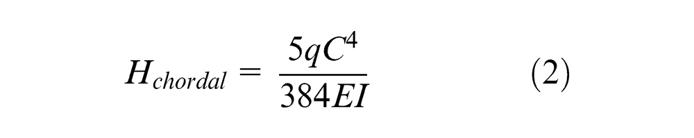
where q is the uniform load per unit length due to gravity and depends on the angle α between the facet and the horizontal plane:
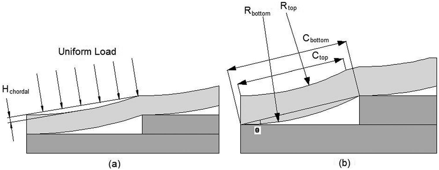
Curved layers over a flat layer structure: (a) filament sagging under a uniform load and (b) geometrical features of the chordal deflection between two successive layers.
Once the first curved layer is deposited, the supports are wrapped around, and the first layer offers a better support for the next layer, thus reducing the subsequent chordal height, as shown in Figure 6(b). The relationship between the first and second chordal heights can be written as
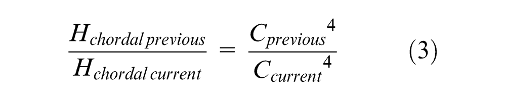
The geometrical relationship between
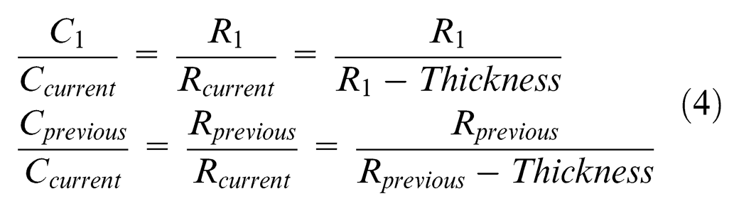
where
Equation (4) could also be used to determine the air gap for the support structure or help determine the quantity of the layer to fill the current air gap in the support structure.
The chordal height is used as follows:
The angle of each facet on the top surface is noted and used with the minimum thickness of the layer to calculate the maximum span. Based on the angle between the facet and a horizontal plane where the maximum span is, the deflection is obtained as the initial chordal height, as shown in Figure 6(a).
Once the initial chordal height is obtained, the top surface is offset to form the curved top layer as shown in Figure 6(b). The chordal height from all the facets is calculated and used to get the maximum chordal height.
Then the maximum chordal height is compared with the user-defined chordal error. If the maximum chordal height is greater than the user-defined chordal error, an extra curved layer needs to be used.
This process is repeated until the chordal height meets the requirement to finalise the required number of curved layers.
Once the number of the curved layers is finalised, the bottom layer needs to be offset once to become the top surface of the flat layer region.
Curved layer slicing
Curved layer slicing is achieved by offsetting the intersection point of three reference planes. Each facet belonging to the top surface is chosen to be the reference spatial plane, which can be described as

where

and

when
Considering a matrix [N], where

where

This procedure is repeated with each triangular facet to obtain an offset surface and then from one offset surface to the next, until all the curved layer domains of the CAD model are sliced using curved layers.
Curved layer offsetting: some difficulties
The top-surface information is used to slice the curved layer region using the three-plane method and the resulting curved layers generated based on the sample part are shown in Figure 7. However, considering the facet structure, there are usually problems associated with the offset surfaces, such as discontinuities, as shown in Figure 8. Qu and Stucker 16 noted that discontinuities may arise if more than three normal directions exist at a given vertex, based on the facet structure.
Curved layer slicing.
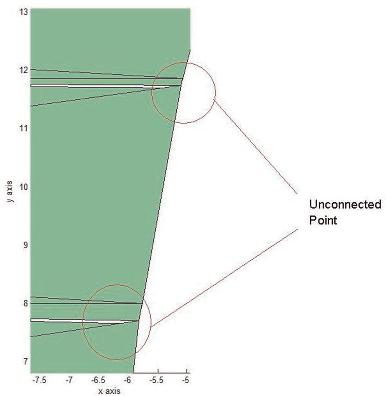
Unconnected points after offsetting.
Analytically, unconnected points arise as follows:
For instance, a point

After offsetting

where [C] is (t, 0, 0)T or (t, t, 0)T or (t, 0, 0)T, depending on the situations as mentioned above
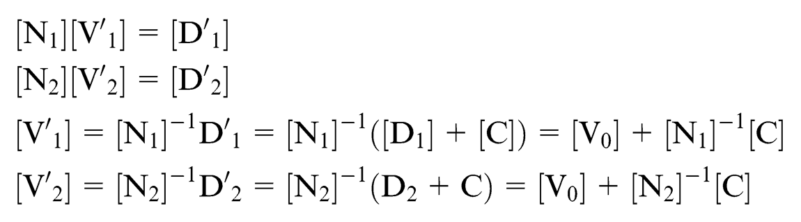
If
Flat layer region
Once the curved and flat layer regions are clearly divided, the flat layer part needs to be reconstructed back into the .stl format file, as conventional flat layers generated based on the whole volume are likely to interfere with the curved layers. The first step of this is to restructure the top surface of the flat layer region, which will also serve as the boundary between the curved and flat layer portions and is generated by offsetting the bottom-most curved layer through one layer thickness. The triangular facets on the side faces also may need restructuring, as most of them get distributed over the two regions, as shown in Figure 9.
Side facets shared between curved and flat layer regions.
Two different methods of reconstruction are used, depending on the complexity of the shape. First, considering a simple solid shape with a curved feature as shown in Figure 10(a), the flat layer portion is reconstructed into a new .stl file, by projecting the top nodes of all side facets on to the boundary surface between the curved and flat regions. Furthermore, the element numbers and connectivity are carried forward from the original .stl file, as these will remain the same, even with the restructured shape of the flat layer portion. After the reconstruction, the coordinates of the top-surface points are modified, and the .stl form of the flat layer portion looks as shown in Figure 10(b). However, this works well only when the offset surface and the top surface of the flat region parts are one and the same.
Flat layer region reconstruction by projecting top-surface points: (a) Original model and (b) reconstruction model.
When the offset surface is not the new reference top surface of the flat region, for example, as in the case of the slightly more complex shape shown in Figure 11, an altogether new .stl format file needs to be built. The part shown in Figure 11 has an irregularly shaped lateral hole, intentionally created to be able to test the effectiveness of the algorithm developed. The algorithm proposed is not a generalised scheme that can process any given shape, but will be able to handle a given solid part with an internal cavity of any shape. Based on a given range of normal directions, all faces of the given solid with a horizontal orientation are identified. In the case of the previous part, there are only two such surfaces, the curved one becomes the top surface and the flat one becomes the bottom surface. In the case of the part with a central cavity or hole, there are four such surfaces. The highest curved surface will be considered as the top surface for the whole part, and the bottom surface of the curved region will be differentiated from the actual bottom surface based on a check using the z coordinates. Once this is identified, the curved region is clearly identified, and the rest of the part becomes the region for flat layer slicing.
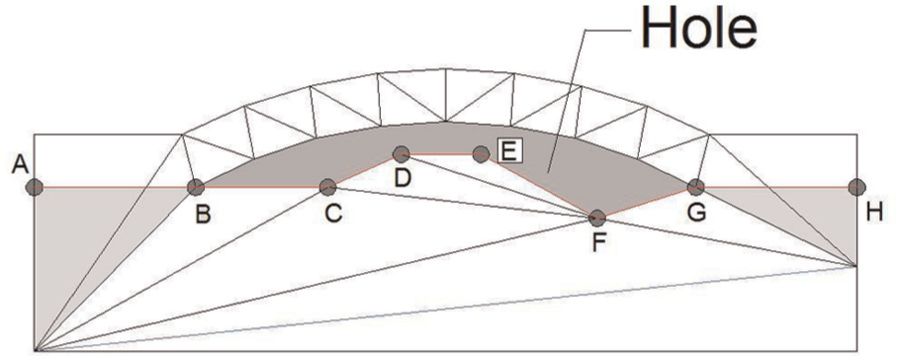
A part with a curved top surface and a lateral through hole.
First, the points on the intermediate surface of the solid together with the points on the boundary between the curved and flat portions of the solid are marked, for example, as points A, B, C, etc. in Figure 11, as seen from the side view of the solid. Once the boundary points are identified, they are divided into two sets: the set that is freshly formed due to a partition between the curved and flat regions, such as points A, B, G and H, and the set that is already existing in the original .stl file, such as C, D, E and F. With the set of pre-existing points, there are triangular facets that are already defined, and they will be used as they are. However, with the new set of boundary points, new facets are generated following the rules of triangulation. Furthermore, the side facets also will be modified only where they are connected to the new points, while other existing facets are used as they are. For example, in the shaded portions on either side of the side view shown in Figure 11, some of the existing facets are deleted and fresh connections are made joining points like A, B, G and H to the bottom corner points. After implementing the algorithm, the curved and flat regions of the part with a central hole are separated and triangulated as shown in Figure 12. After restructuring and renewed triangulation, the flat layer data are generated in similar lines as presented by Lin 17 which usually involves three stages: (1) establishing the intersection profile between the slicing plane and the solid model at the given vertical position, (2) sorting points on the section contour and (3) developing deposition path data for selected raster orientations.
Flat layer region reconstruction by using the existing facets: (a) Original model and (b) reconstruction model.
Case studies and practical implementation
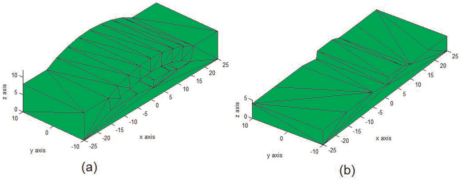
The mixed-mode slicing techniques are implemented in MATLAB and tested for specific cases, using both uniform flat and curved layers. Figure 13(a) and (b) shows the .stl format file form and the combined curved and flat layer slices generated for the full solid part using the current algorithms. It may be seen that the top curved part is modelled with curved layers, while the sold base part is filled with uniform flat layers. The maximum span is 6.995 mm, and the chordal height based on equation (2) becomes 0.001 mm. Considering a maximum deflection of 5% and using equations (3) and (4), it was found that a single curved layer satisfies the required error criterion. However, considering other practical problems, three extra curved layers are used, which will also allow for a shell of sufficient strength to envelop the flat layered core. Once the curved region is finalised, the boundary surface is generated, and the flat layer zone is reconstructed using offset vertices and facet reconnection approaches in this case, considering the relatively simple shape.
Sample part with a curved surface by using projecting top-surface points: (a) CAD model in .stl format and (b) Subdivision into zones and slicing.
As already mentioned, the second test part is similar in shape, but has a lateral through hole of an irregular shape, as evident from the form depicted in Figure 14(a) by the .stl format file. In this case, there are two distinctly different zones: one of the thin shell–type form and the other of a normal slab shape. As evident from Figure 14(b), the algorithm picked up the thin shell–type region to be sliced using curved layers. For the lower part, the boundary surface partly matches with the lower curved layer, while the central portion needs to be freshly constructed. A new parting surface is generated with extra facets, and the lower part is rebuilt in the .stl form and sliced using the uniform flat layer slicing algorithm. The mixed curved and flat layer slices created are shown in Figure 14(b).
Sample part with a curved surface and a cut out feature by using projecting top-surface points: (a) CAD model in .stl format and (b) Subdivision into zones and slicing.
Early research by Mani et al. 6 emphasises the need to properly sequence the deposition styles while using multiple deposition schemes. It may be realised that practical implementation of mixed curved and flat layers also requires some consideration and planning prior to actual deposition. Apparently, both parts considered initially required the flat layer portions to be deposited first, so as to serve as the basis for the curved layer deposition. Using the slice data, the two sample parts are rasterised with 45° orientations as shown in Figure 15, based on deposition path generation algorithms implemented in MATLAB. The deposition path data are properly concatenated to form the appropriate sequence of deposition and converted into G and M codes. This information is further transferred to the Rep G 24 interface of the FDM test bed to physically build the test pieces.
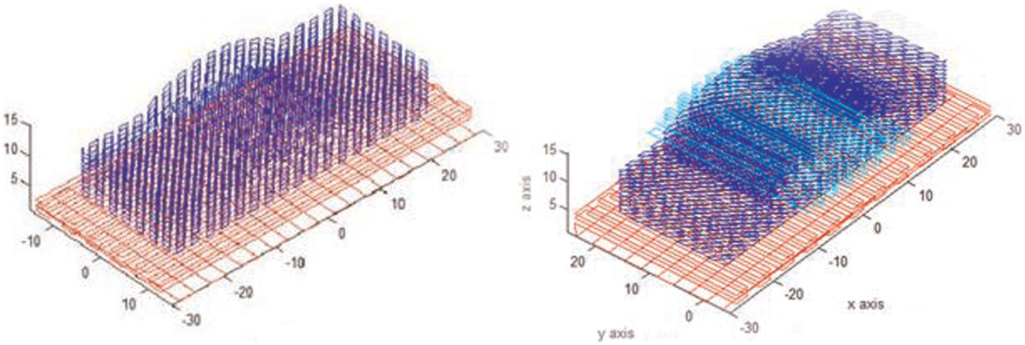
Specimen .stl file is sliced and tool paths generated.
Figures 16 and 17 present photographs of test specimens built with the combined curved and flat layer method. The first one in Figure 16 does not require a support structure, and so the bottom part is printed using flat layers, above which the upper curved form is built using curved layers. However, for the part in Figure 17, the bottom flat layer part is printed first, and then, a sparse support structure is built before laying out the curved layers. While uniform flat and curved layers need 946 and 1409 s, respectively, it was noted that the combined curved and flat layer slicing is a good compromise, requiring 1187 s to build the whole part with better surface quality and internal structure.
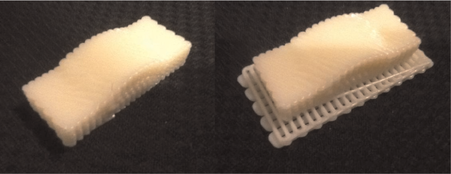
Solid sample part with a curved top surface.
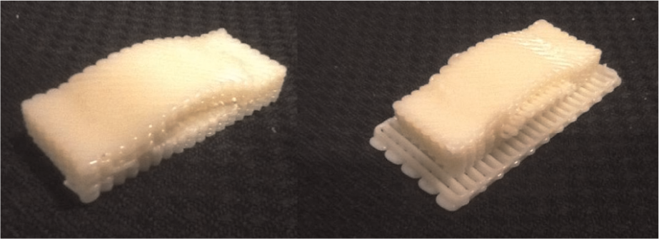
Sample part with a curved top surface and a through hole.
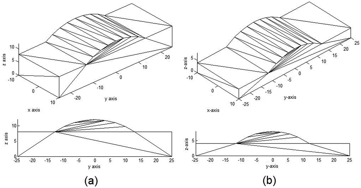
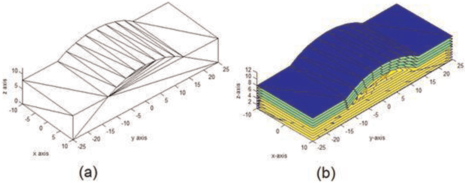
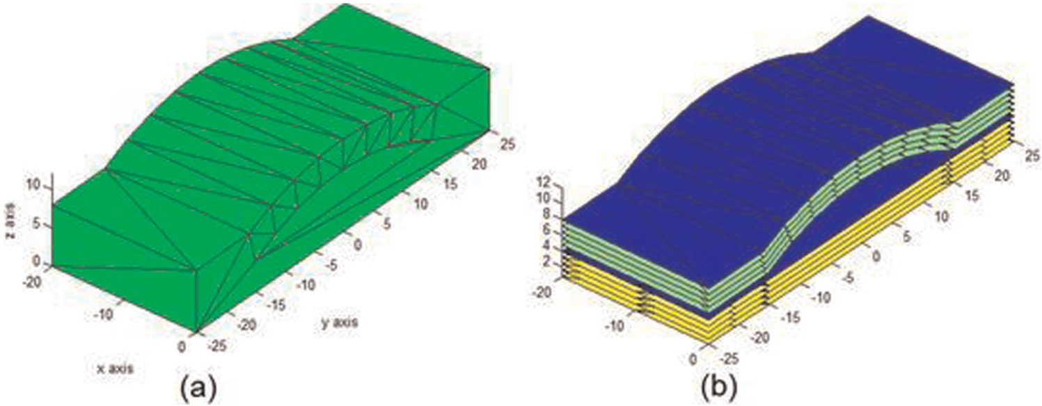
The uniform flat layer and mixed curved and flat layer slicing structures based on the CAD model of the solid part considered as the first case are presented in Figure 18(a) and (b), respectively, while Figure 19(a) and (b) shows the results obtained with the test case 2. Comparing the shaded areas in Figure 18(a) and (b), it may be noted that the stair-step effect is eliminated from the top surface, with the use of curved layers. There is an internal stair-step effect resulting as shown in Figure 18(b) at the boundary between the flat and curved regions, which may be neglected if the part strength is not of significance. In cases calling for both surface and part qualities, use of adaptive flat layers will become essential, but with proper synchronisation of time and speed of printing layers of varying thicknesses. Based on CAD models, it could be evaluated that there is a loss of 4.4% of volume for the case as shown in Figure 18(a). Out of this, 4.1% is due to surface irregularities highlighted in Figure 18(a), while the remaining loss is due to the other areas. And the total volume lost is around 8.5% for the case in Figure 19(a). The mixed distribution in Figure 18(b) allows complete elimination of the stair-step problems on the top surface, but still suffers due to errors at the boundary between flat and curved layers, although the use of adaptive flat layers will allow for a reduction in this error to a large extent. While these are aspects for future investigations, the layer structure obtained by the mixed curved and flat layer slicing for the second solid as shown in Figure 19(b) eliminated the stair-step effects altogether, as compared with the uniform flat layer counter-part of Figure 19(a). Furthermore, use of curved layers in certain zones allowed better fibre continuity as well as elimination of weak inter-layer shear-sliding zones.
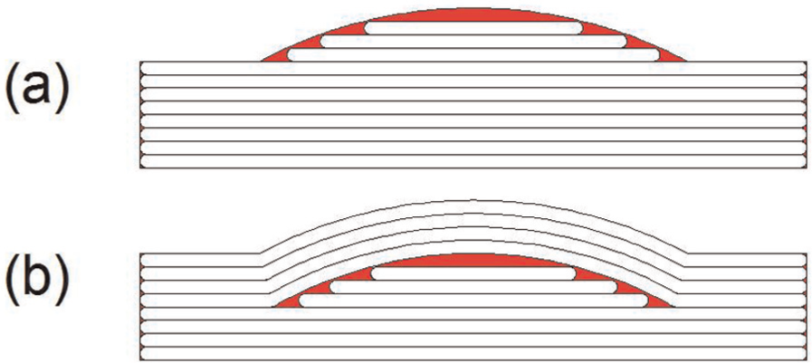
Layer structures in the solid sample part with a curved top surface: (a) uniform flat layer slicing and (b) mixed curved and flat layer slicing.
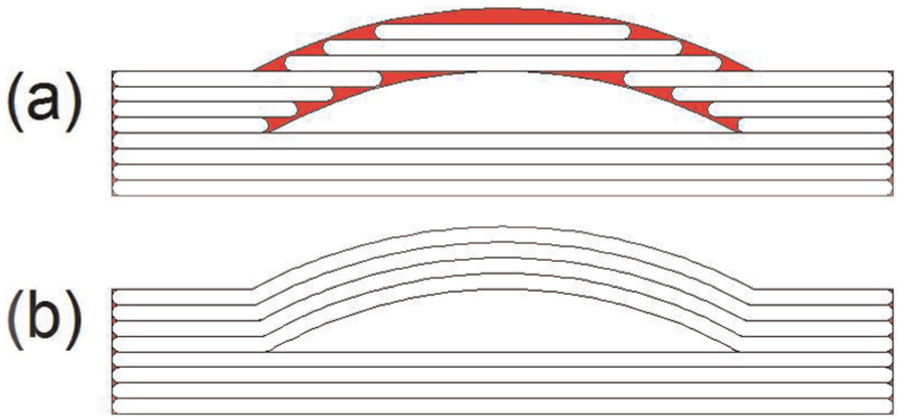
Layer structures in the sample part with a curved top surface and a through hole: (a) uniform flat layer slicing and (b) mixed curved and flat layer slicing.
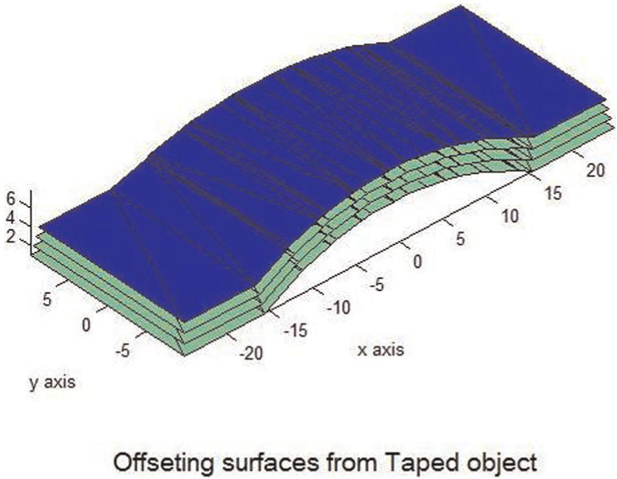
An aircraft wing geometry is considered next to evaluate the effectiveness of the mixed slicing algorithm. Although direct digital production of aircraft wing structures is far from reality at present, AM methods are commonly used to produce functional wing models for aerodynamic analyses. As presented in Figure 20, the aircraft wing consists of curved surfaces both at the top and the bottom as against having a flat base as with the other two cases. Uniform flat layer slicing in this case will result in stair-step effects on the entire outer surface, resulting in a clear loss of the aerodynamic attributes. The geometry of the aircraft wing analysed is shown in Figure 21(a) in .stl format.
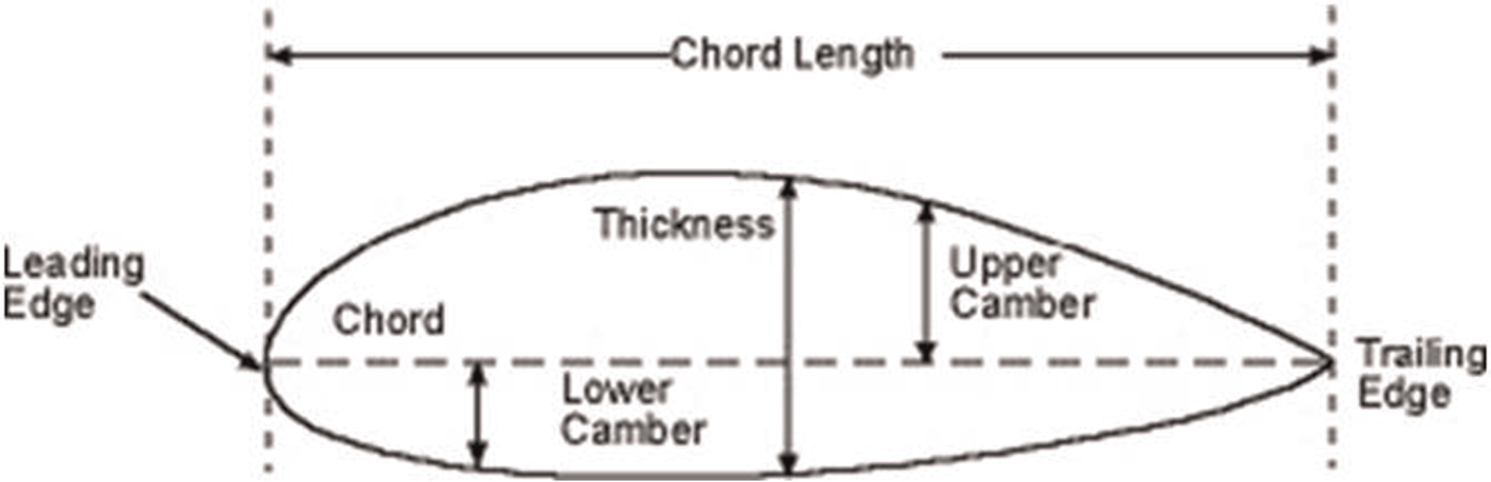
Aircraft wing cross-section.
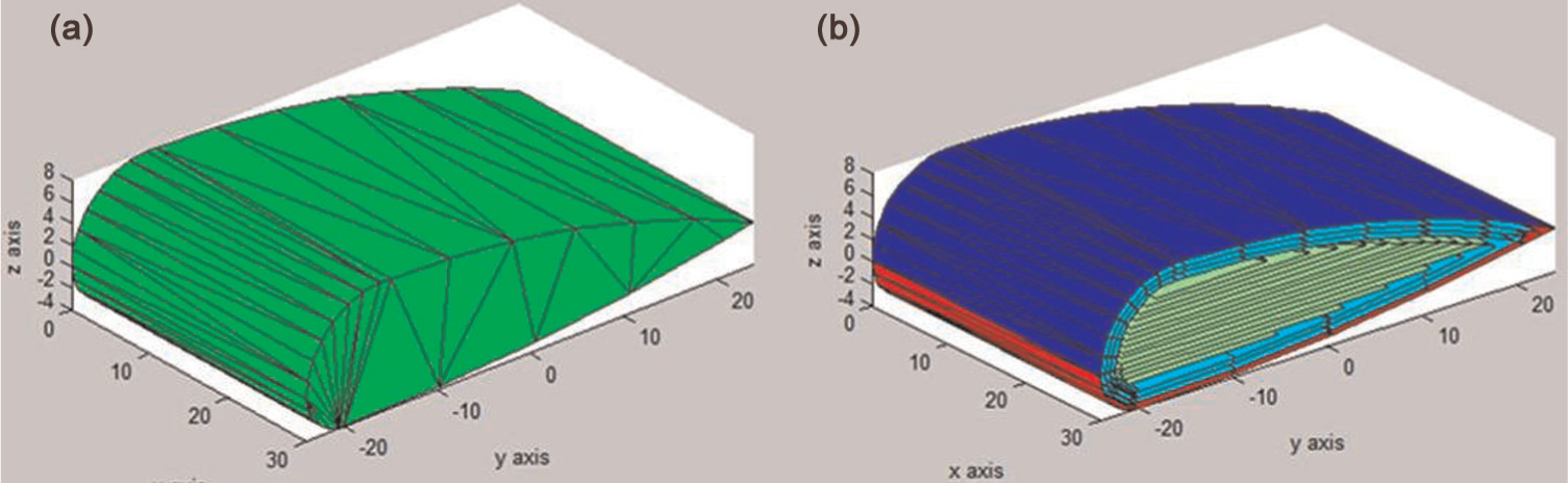
Mixed-layer slicing applied to the aircraft wing geometry: (a) the .stl format file and (b) curved layer skin and flat layer core.
When the mixed-layer algorithm is applied to this part, the need for curved layer slicing close to both the top and the bottom surfaces is identified, while the interior is filled with uniform flat layers. In this case, the algorithm first divides the part into two volumes based on a central plane considered passing through the two extreme points. The external curved surfaces of the top and bottom parts are then identified as the key surfaces. Sets of points generated on these two surfaces are then used to construct the offset layers, and a few curved layers are generated from both surfaces as shown in Figure 21(b), based on the chordal error considerations. Once the boundary surfaces are identified, the interior is filled with uniform flat layers. It may be noted that the curved layers at the bottom may require a support structure below the overhanging curved portion.
Conclusion
A combined curved and flat layer slicing approach is proposed and implemented in this research for FDL. Mathematical algorithms are developed based on .stl format files. The chordal error evaluation method was effective in dividing the solid model domain into curved and flat layer regions. The mixed-layer approach usually takes more time to print compared to the uniform flat layer approach, but the surface and internal meso-structure are much improved. The three-plane-intersection approach is able to create curved slices, while there are existing solutions for the flat layer counterparts. The algorithms developed are successfully integrated and tested with a couple of examples requiring both curved and flat layer slices, and the concatenated deposition path profile was used for practical implementation of the mixed-layer deposition on a test bed. The mixed slicing approach is effective in eliminating the stair-step effects either partly or completely, depending on the geometry of the part.
Footnotes
Declaration of conflicting interests
The authors declare that there is no conflict of interest.
Funding
This research received no specific grant from any funding agency in the public, commercial or not-for-profit sectors.