
Abstract
This article focuses on identifying and fully utilizing the dynamic capabilities of a nanopositioning system to optimally trace a given trajectory. This work develops a framework for abstracting the capabilities of the piezo-actuated nanopositioning systems and a methodology for using these capabilities to generate an optimal trajectory for a particular tool path on a given nanopositioning system while satisfying all the process-related requirements. Several dynamic capabilities of a typical nanopositioning system are identified and modeled as the constraints to drive the optimization problem. First, the velocity and acceleration capabilities of each individual axes are constrained by developing a simplified dynamic model of the performance envelope, which couple velocity and acceleration capabilities of each axis, as a function of displacement. Second, input command bandwidth constraints are introduced to mitigate frequency-related tracking difficulties encountered when traversing sharp geometric features at high velocity. Finally, the accuracy requirement is satisfied by developing a dynamic model of the instantaneous following error to estimate the contour error as a function of the velocity and acceleration at each moment. The above constraints are incorporated into a computationally efficient two-pass algorithm to generate a minimum time feedrate profile for a particular positioning system for any given trajectory. Linear zigzag and cubic spline airfoil trajectories are used to demonstrate the significant improvements in time and contouring accuracy realized through such an approach.
Introduction
With rapid developments in micro/nanotechnology, the micro/nanomanufacturing systems need to satisfy the requirements arising from micro/nanotechnology applications. The research community has spent a lot of effort in developing advanced and sophisticated feedback control techniques to improve the performance of the nanomanufacturing systems. However, such controllers and control algorithms are incapable to provide good performance when the dynamic capabilities of the system are not fully understood and addressed. Performance of such systems will suffer when they are demanded to execute commands beyond their capabilities, especially when following highly complex trajectories. Trajectory planning is the cost-effective approach to ensure that infeasible commands are never requested of each individual axes by the path interpolator. Besides the concern for precision and accuracy, the cycle time or production time is also an important measure of manufacturing performance. These parameters can be improved only if the capabilities of the system are fully exploited.
For conventional scale manufacturing machines, several researchers have addressed the time-optimal trajectory control problem by ensuring that the actuator was always within its capabilities. Lynch 1 developed a specialized minimum time algorithm assuming constant bounds for the actuators. This assumption is prone to over-constrain the system and was improved by Bobrow et al. 2 where they came up with a solution to find acceleration profiles such that at each acceleration point, the actuator delivers the maximum velocity possible which is not greater than the maximum capability delivered by the actuator. Shin and McKay 3 presented a computationally intensive algorithm where the bounds on the actuator were described by a quadratic function of an actuator’s parameter.
Most of the optimization approaches have produced exemplary results with respect to time, but not much work has been done in the literature to confine the contouring accuracy within a given tolerance limit. Dahl 4 accounted for the modeling errors and real-time disturbances by implementation of a path velocity controller outside the ordinary robot controller. Cao et al. 5 approached the time-optimization path planning problem by optimizing the movement of the robotic joint paths rather than that of the end-effector. Many other researchers achieved the control at the trajectory planning stage or optimization stage instead of handling them with a real-time controller. Zlajpah 6 focused on a solution to the optimal trajectory planning subject to joint torque constraints, joint velocity constraints and task constraints. Many other constraints were also used in trajectory control problems, such as constant torque limitations 7 and constraints on the acceleration and retardation time. 8 Imamura and Kaufman,9,10 in addition to optimizing the contouring time through nonlinear programming techniques, tuned the controller subject to the actuator power constraints. In Amthor et al.,11,12 an analytical trajectory generation method was developed to plan trajectory under many dynamic state constraints from velocity to jerk.
To solve the optimization problem to obtain the optimal solution, many approaches have been developed. Butler and Tomizuka 13 approached the problem analytically for machine tools through the solution of a differential equation rather than through the solution to an optimization problem. Farouki et al. 14 developed an analytical model to determine the safe fixed feedrate along a curved tool path and safe rates of increase in feedrate with time or arc length. Pfeiffer and Johanni 15 transformed the equations of motion for the manipulator into a parametric variable resulting in an ordinary differential equation containing the dynamics of the manipulator like path acceleration, velocity and many other parameters. Such analytical approaches had computational inefficiency for trajectories with complex geometries. Most of them also lack the flexibility to include extra parameters or constraints that arise from different systems or process requirements. Renton and Elbestawi 16 have developed a computationally efficient two-pass algorithm to solve the feedrate optimization problem. The algorithm scans the trajectory twice. The forward pass tries to scan the trajectory in an optimum time and the reverse pass tries to remove infeasibilities like sudden reversals or changes in acceleration. Dong and Stori17,18 and Dong et al. 19 developed a feedrate optimization algorithm using a bi-directional scan structure accounting for any dynamic state–related constraints and proved the optimality of the algorithm. Other researchers20–22 formulated the trajectory control as a mathematic programming problem and solved it analytically using dynamic capabilities and tracking error constraints.
Most of the previous works for the trajectory control problem focus on finding the capability bounds of conventional scale manufacturing machines, in which electrical motors are used as actuators. However, these works cannot be extended to piezo-actuator systems used in micro/nanopositioning systems, whose dynamics are dependent on the specific displacement or position of the actuator. In contrast to conventional scale motor-driven manufacturing machines, nanomanufacturing systems are mostly flexure-based piezo-driven systems. The capabilities of the piezoelectric actuator and the behaviors of the nanomanufacturing systems are very different from the conventional scale manufacturing systems in their dynamic capabilities of velocity and acceleration in the actuator system. 23 Moreover, for micro/nanomanufacturing applications, accuracy concerns are critical, which can be achieved only through careful planning efforts along with closed-loop controllers. Most of the commercial manufacturing machines have impressive claims regarding the speed and accuracy, but fail to guarantee a maximum error limit, such as the maximum contouring error that can be expected for a given complex trajectory. This article addresses the accuracy concerns by taking it into account at the optimization stage.
In this work, we identify the dynamic capabilities of a typical nanopositioning system actuated by piezoelectric actuators. 24 The system capabilities and the accuracy requirements are expressed by a set of constraints to drive the minimum time trajectory control problem. A feedrate optimization algorithm is used to generate the optimal feedrate profile for the nanopositioning system to execute a particular trajectory. The resulting time-optimal (minimum time) trajectory fully utilizes the dynamic capabilities of the nanopositioning system while maintaining the specified contouring accuracy. Detailed experimental results are presented demonstrating the improvements in contouring accuracy that can be achieved through the use of such an optimization approach to the feedrate scheduling problem.
Modeling constraints from actuator limitations and accuracy requirements
Constraints from actuator limitations
Piezoelectric actuators and high-resolution displacement sensor (e.g. capacitive gage) are widely used in nanopositioning systems to obtain displacement with nanometer resolution. Irrespective of the mode of actuation, all these actuators have limitations in their output force and power capabilities. If the actuators are commanded to deliver velocities or acceleration beyond their capabilities, the performance of the overall system will be degraded and a large tracking error and contouring error will be observed. These kinds of errors cannot be modeled and compensated solely by a stand-alone feedback controller. We need to identify the capability or feasible region of the device, so that the controller does not request velocities and accelerations beyond the device’s capabilities.
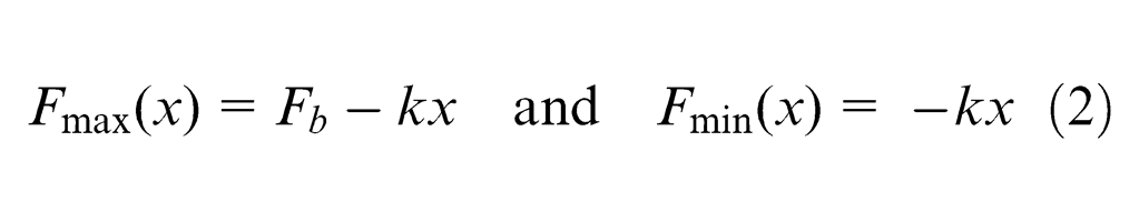
Piezoelectric ceramics driven by electric fields are widely used in nanopositioning systems due to their fast response and large force output. The total displacement that can be provided by a piezoelectric actuator is quite limited, roughly from a few microns to tens of microns. The special characteristic of the piezoelectric actuator is that the maximum actuation force is position dependent. When there is no displacement output from a piezoelectric actuator, it offers the maximum force output, called the blocking force. However, when the actuator is at its maximum displacement, it is not capable of providing any output force. The driving capability of a piezoelectric actuator is determined by its maximum displacement without load, also referred to as free stroke Sf , and blocking force Fb = Fmax . There is a linear relationship between the actuation force and the displacement of the actuator for a given driving voltage V, as shown in equation (1)
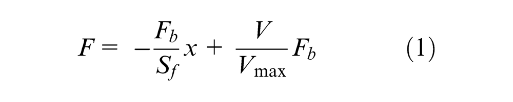
where F is the force output, x is the displacement output and V
max is the maximum driving voltage, as shown in Figure 1. The term
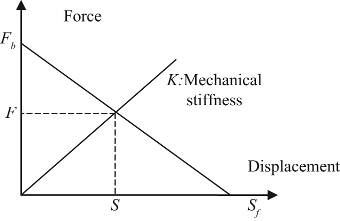
Displacement–force relationship of piezo-actuators considering structure stiffness.
where
In general, a second-order model should be sufficient to capture the majority of the low-frequency dynamic behavior of a single axis of a typical manufacturing machine. From the trajectory planning point of view, we are interested in the relationship between the constraints of the physical system and the corresponding feasible dynamic states including displacement, velocities and accelerations for each axis
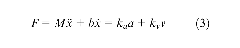
The maximum actuator torque or force will be the primary system constraint. From equation (3), we can see that a linear combination of the acceleration and velocity of each axis must be constrained at all times
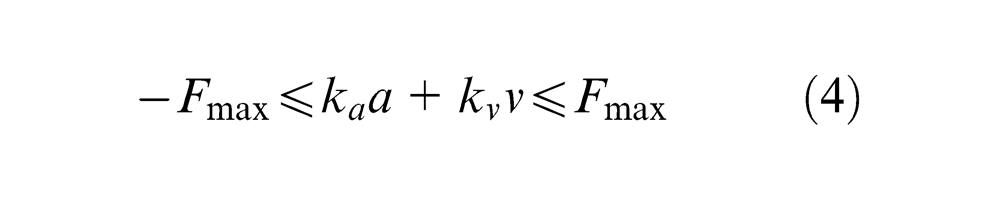
where the constants ka and kv represent the inertia and viscous characteristics of a particular axis, respectively.
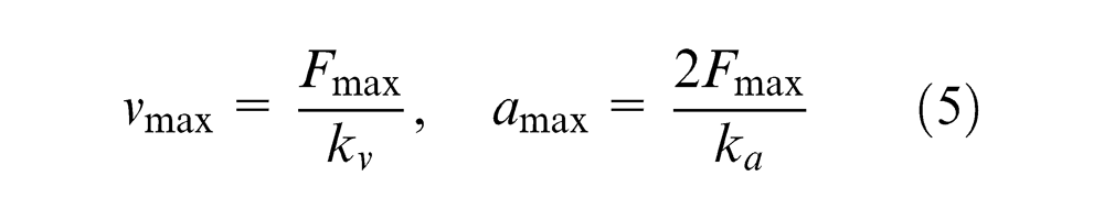
Under the assumption of such an ideal second-order dynamic system with a fixed actuator output and constant inertial and viscous force coefficients, the maximum feedrate or speed is achieved when all the driving force is used to overcome the viscous force. At this velocity, there will be no acceleration possible in the forward direction. However, at this maximal forward velocity, the reversed acceleration will be maximized
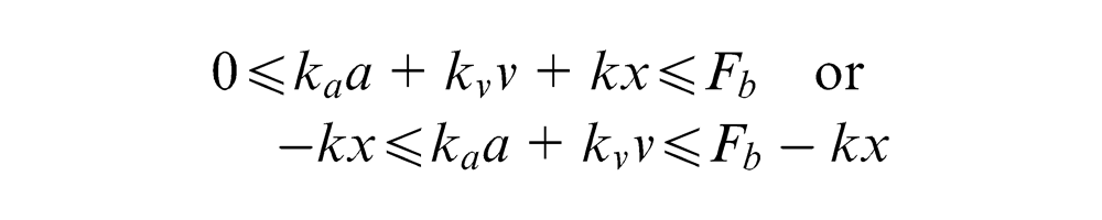
When the actuation force is displacement independent (e.g. in motors), the above constraints result in a feasible parallelogram within the acceleration versus velocity space for a particular axis (Figure 2(a)). However, for a piezoelectric actuator, since its actuation force depends on its displacement, the acceleration capability will be more complex. Equation (4) can be extended as
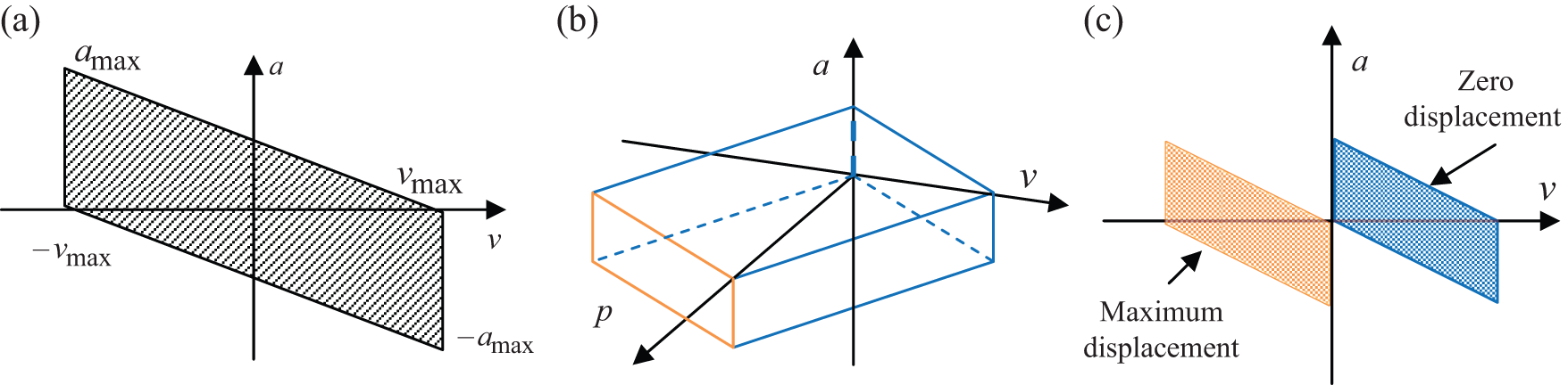
(a) Parallelogram constraints for electrical motors with displacement-independent actuation force. (b) Capability envelope of a piezo-actuator in the space of position–velocity–acceleration. (c) Projection to v–a plane when at 0 and maximum displacement.
The capability boundary is described in the three-dimensional (3D) space of position–velocity–acceleration (Figure 2(b), instead of the two-dimensional (2D) space of velocity–acceleration of motor systems. The performance envelope shifts from right to left on v–a plane as the displacement increases, due to the term kx in the constraint. Initially, when the actuator is at rest, that is, x = 0, the actuator cannot move in the negative direction. The minimum velocity, that is, the maximum reverse velocity is 0 and this makes the maximum reverse acceleration to also be 0 since the actuator cannot displace in that direction. The maximum forward acceleration is at its maximum at zero velocity. Now the maximum forward velocity is achieved when all the driving force is used to overcome the viscous force. The velocity–acceleration feasible region for the initial position of the actuator takes the form shown in Figure 2(c). For the end position of the actuator along a particular axis, the entire driving force is spent in reaching the maximum displacement, which gives rise to the conclusion that the maximum forward velocity for the actuator when it is in its maximum displacement position is 0. Hence, the maximum forward acceleration is also 0 and the reverse acceleration or deceleration is maximized. The velocity–acceleration feasible region shifts to the left half of v–a plane. Overall, a 3D feasible space can be used to describe the capability of the piezoelectric actuator-driven nanopositioning system. The model parameters can be estimated by model identification to fit the second-order models, as shown in equation (3).
Input command bandwidth constraints
Although control engineers are very much aware of the closed-loop bandwidth of the entire system during design and tuning of control loops, there is no assurance that the future commands, in the form of geometrically complex high-speed trajectories, will not contain larger frequency components in excess of the system capabilities. Since when planning the trajectory and scheduling the corresponding feedrate profile, the path geometry is known beforehand, it is possible to constrain the input command signals so that the dominant frequency content of the input command is always below the pre-selected constraints of the frequency tracking abilities of each individual axes.
The dominant frequency requested of an individual axis can be estimated at each point along the trajectory from the path curvature and the velocity scheduled at that point. We can derive the instantaneous path curvature and use the tangent velocity identified by the feedrate scheduling algorithm to calculate the dominant frequency that will be experienced by each of the individual axis. The dominant frequency of magnitude ω is then found from the following equation

This limiting bandwidth of each individual axis is different from the closed-loop bandwidth of the system, and in most of cases significantly lower than the closed-loop bandwidth. The widely used closed-loop bandwidth for a control system is not a suitable value for the input command signal bandwidth constraint to ensure contouring accuracy, since by definition it would permit the radius of a representative circle to shrink by about 30% at the worst case. The frequency content of the command signal following this input command bandwidth constraint will be considerably lower than the frequency of signals that can be tracked by the controller. This constraint will be important in traversing sharp curves and turns as it is a function of the path curvature.
Constraints on contour accuracy
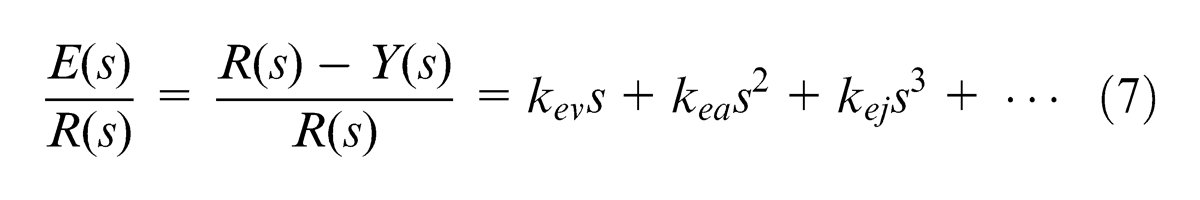
The whole goal of exploiting the capabilities of the physical system is to contour the trajectory in minimum time possible but definitely not at the cost of accuracy. Designing and tuning of control loops will improve the accuracy and performance but might not satisfy the optimum time requirements. Hence, to have a trajectory scanned at an optimum time with significant level of accuracy, we need to estimate the contour error at the feedrate scheduling stage as a function of the system dynamic states, such as position, velocity and acceleration. In this section, dynamic models of the closed-loop system of each individual axes are developed and utilized to predict the instantaneous contour error. To estimate the tracking accuracy of the desired axes, we can derive the closed-loop error transfer function from the dynamic model of the machine G(s) and the unit feedback closed-loop controller K(s). The error transfer function can be expressed as
The above expression can be converted to time domain to estimate the following error as a function of instantaneous velocity and acceleration. The convergence is uniform on any closed subdisk
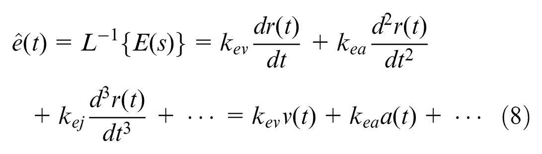
Expression (8) provides an estimate of the tracking error as a linear combination of the dynamic error coefficients and the instantaneous velocity and acceleration. To simplify the computations, we neglect the terms of order higher than acceleration in the prediction of the following error.
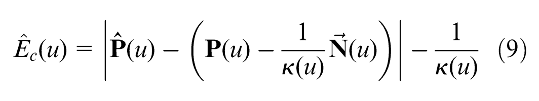
The predicted following error will now be used to estimate the contour error at all instants, and hence this can be constrained to achieve required contouring accuracy. A relation between the instantaneous velocity, acceleration and the path contouring error can be derived. Numerous researchers have estimated contour error through real-time feedback control techniques. Since the geometry of the trajectory is not known a priori to the real-time controller, the most common approach relies on tangential approximation to the path geometry. In our case, using the methods discussed in Dong and Stori,
17
we use the curvature circle approximation to estimate the contour error. Figure 3 shows the methods of estimating the contour error. In Figure 3, the vector P(u) represents the target position, u is the variable that parametrically represents the trajectory given in Cartesian coordinates,
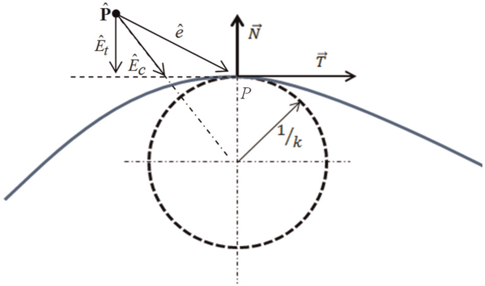
Tangential and curvature-based estimates of contour error.
where
Feedrate optimization using bi-directional scan algorithm
A given parametric trajectory
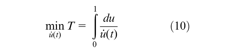
subject to
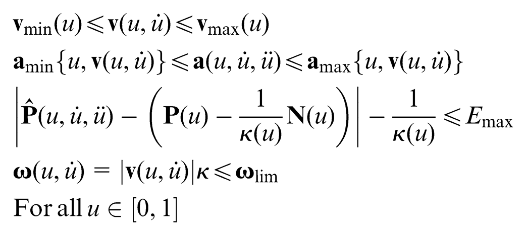
In the optimization problem expressed in equation (10), a parametric trajectory function u(t) is to be determined such that the entire trajectory is executed in minimum time and the constraints specify that the dynamic capabilities of the individual axes must be observed at all times satisfying the contour error requirements as well.
For this work, we utilized the bi-directional optimization algorithm that Dong and Stori17,18 developed. We applied the constraints we developed for a typical micro/nanomanufacturing system. The algorithm provided works based on a series of single variable optimization subproblems that may be efficiently solved using traditional line-search techniques.
The algorithm is a bi-directional scan algorithm with scans, namely, forward scan and backward scan. The minimum time feedrate scheduling algorithm begins with the forward scan, where all the segments and hence the parametric points in each segment are scanned in the forward direction. The optimization problem shown by equation (10) is solved for each such parametric point for the optimal feasible values of parametric velocity at each point. If the problem is infeasible, we reduce the parametric velocity of the previous point until feasibility is obtained and all the constraints are satisfied. During the forward scan, a trajectory is generated that attempts to minimize the time at each step by either accelerating to its maximum possible or maintaining the maximum possible velocity, subject to the constraints on each axis’s capabilities. This component of the algorithm is “greedy” in that the local velocity is maximized, regardless of the potential future repercussions. As a result, the existence of a feasible solution to this system is not guaranteed throughout the trajectory. In general, this strategy can lead to points at which the acceleration capabilities are insufficient to maintain the required path geometry or achieve a decreased velocity dictated by bandwidth considerations.
The backward scan accounts for making the above solution feasible by imposing deceleration constraints and reducing the velocity and still holding it continuous. During the backward pass, through the algorithm, the infeasibilities are removed. This reverse scan is continued until the beginning of the trajectory is reached. Discontinuities in the forward pass result from a large accumulated velocity that is “blind” to an approaching trajectory transition. In the reverse pass, the parametric velocity is constrained to never exceed the velocity assigned during the forward pass, and hence, a feasible solution will always exist. By traversing through the trajectory in the reverse pass, deceleration feasibility is ensured.
The structure of this algorithm is well-suited to the addition of state-dependent constraints. At the end of the feedrate scheduling algorithm, a time-optimum trajectory is obtained that satisfies all the required constraints. The optimization procedure will generate continuous parametric velocity profile and parametric acceleration profile that is piecewise continuous. The algorithm developed and the approach used can be easily implemented and interfaced with any of the commercially available interpolators and positioning stages. The experimental results will demonstrate the improvements obtained through such an upper-level of trajectory control.
High-speed nanopositioning systems as the testbed
In this study, we used a high-bandwidth parallel kinematic stage designed and developed by Polit and Dong 24 as a test platform to carry out experimentation and obtain experimental data. The stage has two axes and each axis is composed of three doubly clamped beams and a parallelogram hybrid flexure with complaint beams and circular flexural hinges. The mechanical design decouples the motion along each axis making the axis function independently and restricts parasitic rotations in the xy plane while allowing for linear kinematics in the operating region. These characteristics of the positioning platform help achieve a uniform performance across the workspace. The stage is actuated by piezoelectric stack actuators and capacitive-type proximity sensors were added to the system to build a closed-loop positioning system. The stage was recorded for a displacement capability of 15 μm along each axis with a resolution of 1 nm along each axis. The image of the stage is shown in Figure 4(a) and its schematic mechanism diagram displayed in Figure 4(b) with the x-axis is actuated. A critically damped linear proportional + integral (PI) controller was developed to close the control loop. The main reason to have critically damped controller and avoid the under-damped controller is the “overshoot.” Although the system was still stable, the under-damped controller gave unsettled oscillations within the set value. Even small oscillations can make high-precision tracking unacceptable; the results of using the under-damped controller are shown in Figure 5.
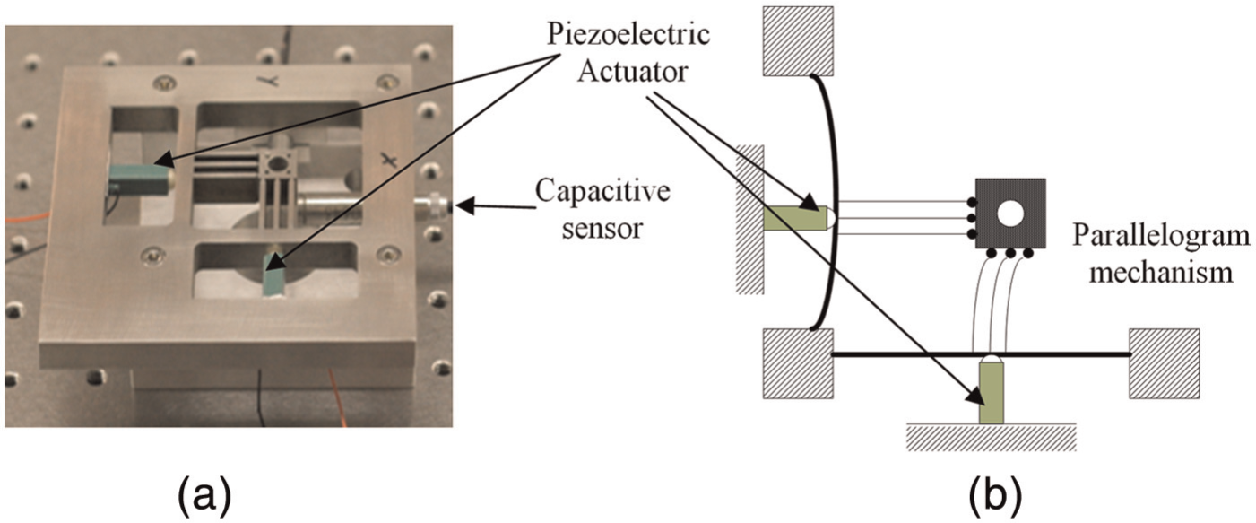
(a) Parallel kinematic nanopositioning xy stage as the testbed. (b) Schematics representation of the xy stage (deformed system when x-axis is actuated).
Effects of overshoot and oscillatory response of an under-damped controller.
This oscillatory response was noted in tracing linear trajectories as well which made the under-damped controller a highly undesirable one. For high-performance contouring, such oscillations or overshoot will produce adverse results which will reduce the effects of the feedrate scheduling and optimization. The error coefficients in equation (8) are identified experimentally by given different constant velocity trajectories and constant acceleration trajectories and analyzing the resulting tracking error of each axis. Figure 6 compares the observed following error of each axis with those predicted by the model developed in equation (8) for an airfoil-shaped trajectory shown in Figure 7(b). As may be observed in the figures, the primary trends are well captured. Normally, models similar to the one developed in section “Modeling constraints from actuator limitations and accuracy requirements” are developed under the assumption that the system is operating in its linear region and has no controller or amplifier saturation. In our case, this condition will always be satisfied because of the operation of the actuator within its performance envelope, developed as a constraint in section “Modeling constraints from actuator limitations and accuracy requirements.”
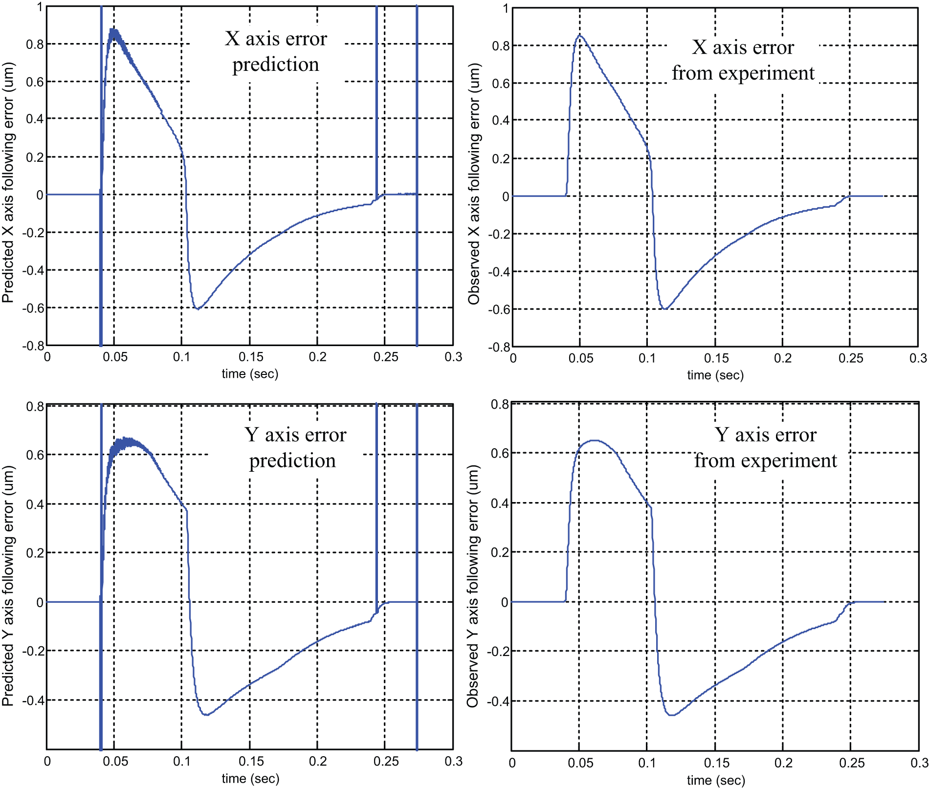
Comparison of tracking error model predictions and experimentally observed following error on airfoil-shaped trajectory shown on the right of Figure 7.
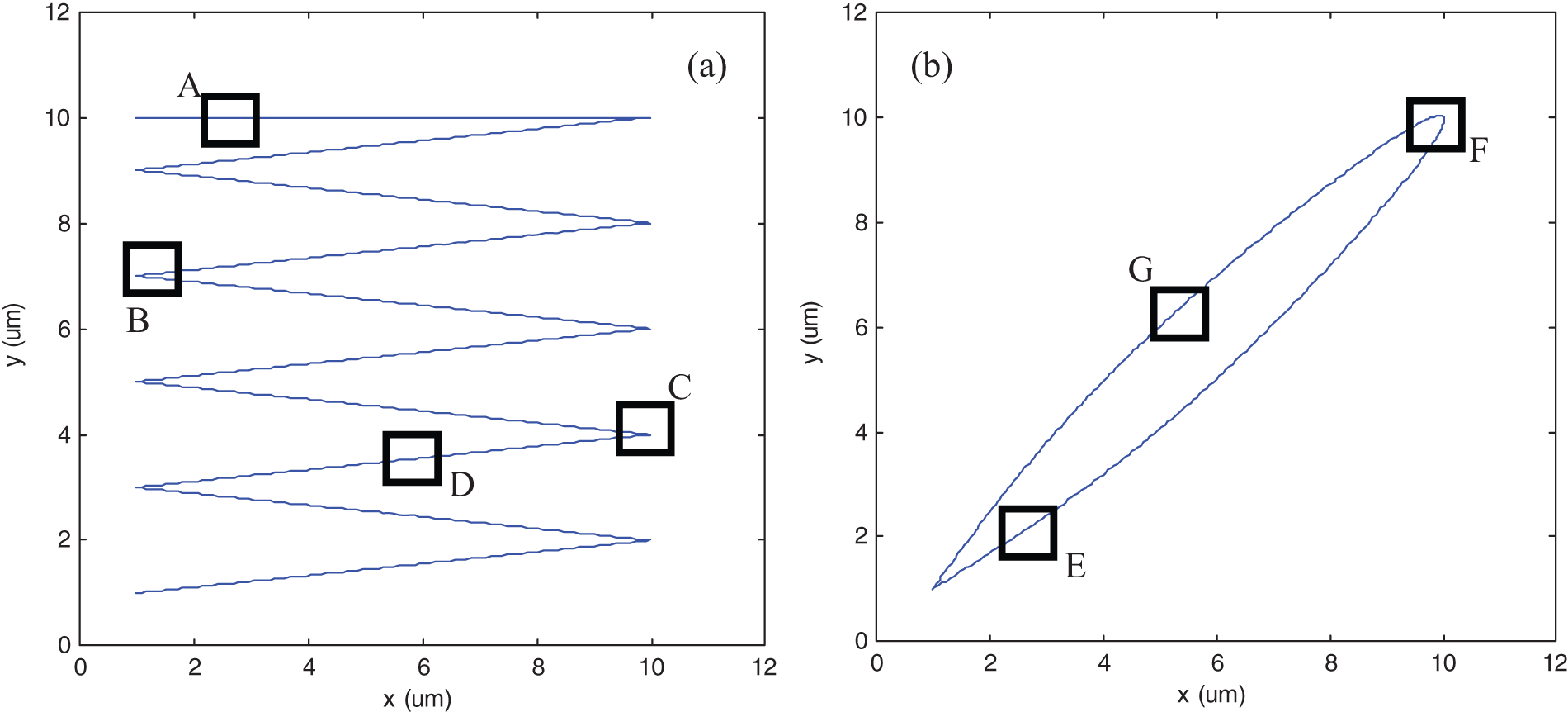
Two test trajectories for case studies. (a) a zigzag linear trajectory. (b) a spline airfoil trajectory.
Experimental validation and case studies
In this section, we present the case studies to evaluate the effectiveness of the feedrate scheduling approach for nanopositioning systems. The test trajectories are a zigzag linear trajectory shown in Figure 7(a), which is a widely used path for image scanning in atomic force microscope, and a spline airfoil trajectory to make the system traverse complex paths shown in Figure 7(b). The test trajectories test the positioning stage through a variety of motions like sharp velocity reversals of x-axis when y-axis is moving at low velocity (regions C and B), simultaneous reversal of both x- and y-axes (region F) and the other parts of the trajectories include horizontal (region A) and diagonal (region D) and nearly diagonal (regions E and G) periods. The full trajectory requires the x–y stage to accelerate from rest, traverse the path and return to rest in minimum time.
The focus of the feedrate optimization is to make full efficient usage of the positioning stage and make improvement in accuracy and contouring time compared with conventional interpolation and constant velocity techniques. We provide the results from the optimization algorithm for two trajectories to illustrate the effect of the constraints. For the zigzag trajectory shown in Figure 7(a), we use constraints from the actuators only. Since the trajectory is linear, it has no curvature component, and hence the frequency constraint and the contour error constraint cannot be applied. Figure 8(a) shows the obligation of the actuator constraints to all points in the trajectory. As expected, the points in the feasible region are such that each point is either at maximum acceleration boundary or maximum velocity boundary of either x- or y-axis, thus constraining the performance of the actuator within its limitations. Figure 8(c) and (d) shows the above explanation visually. Since x-axis is the fast moving axis, the constraints from x-axis are tight constraints. Figure 9 compares the contouring result for the optimization algorithm and constant feedrate (G-code) method. Significant differences can be observed in contouring accuracy due to the approach of trajectory planning and feedrate optimization. At the sharp corners, optimized trajectory can give much better contouring accuracy compared with traditional constant speed trajectory (0.186 vs 0.041 μm).
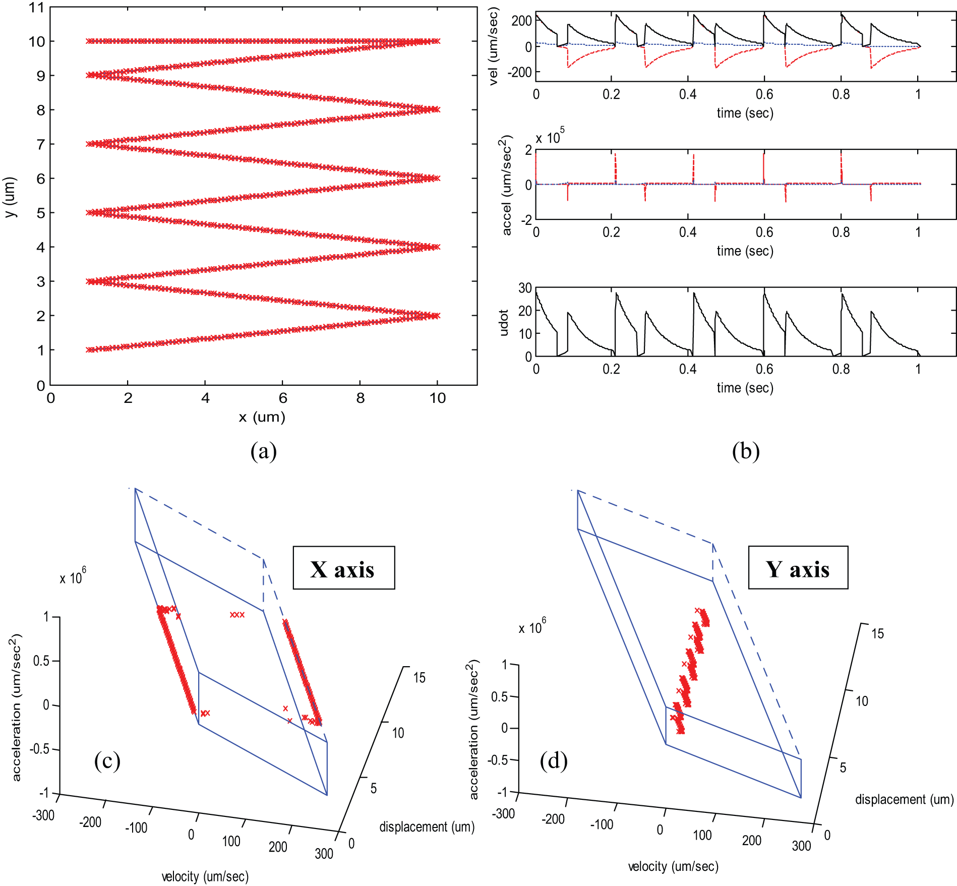
Optimal feedrate scheduling for linear trajectory with actuator constraints only: (a) actuator constraints are satisfied at all points on the trajectory with one of them being satisfied with strict tolerance; (b) velocity, acceleration and parametric velocity profiles (solid line is tangential, dashed is x-axis and dotted is y-axis) and (c, d) performance envelope for each axis showing the strictly satisfied constraints along all the points of displacement.
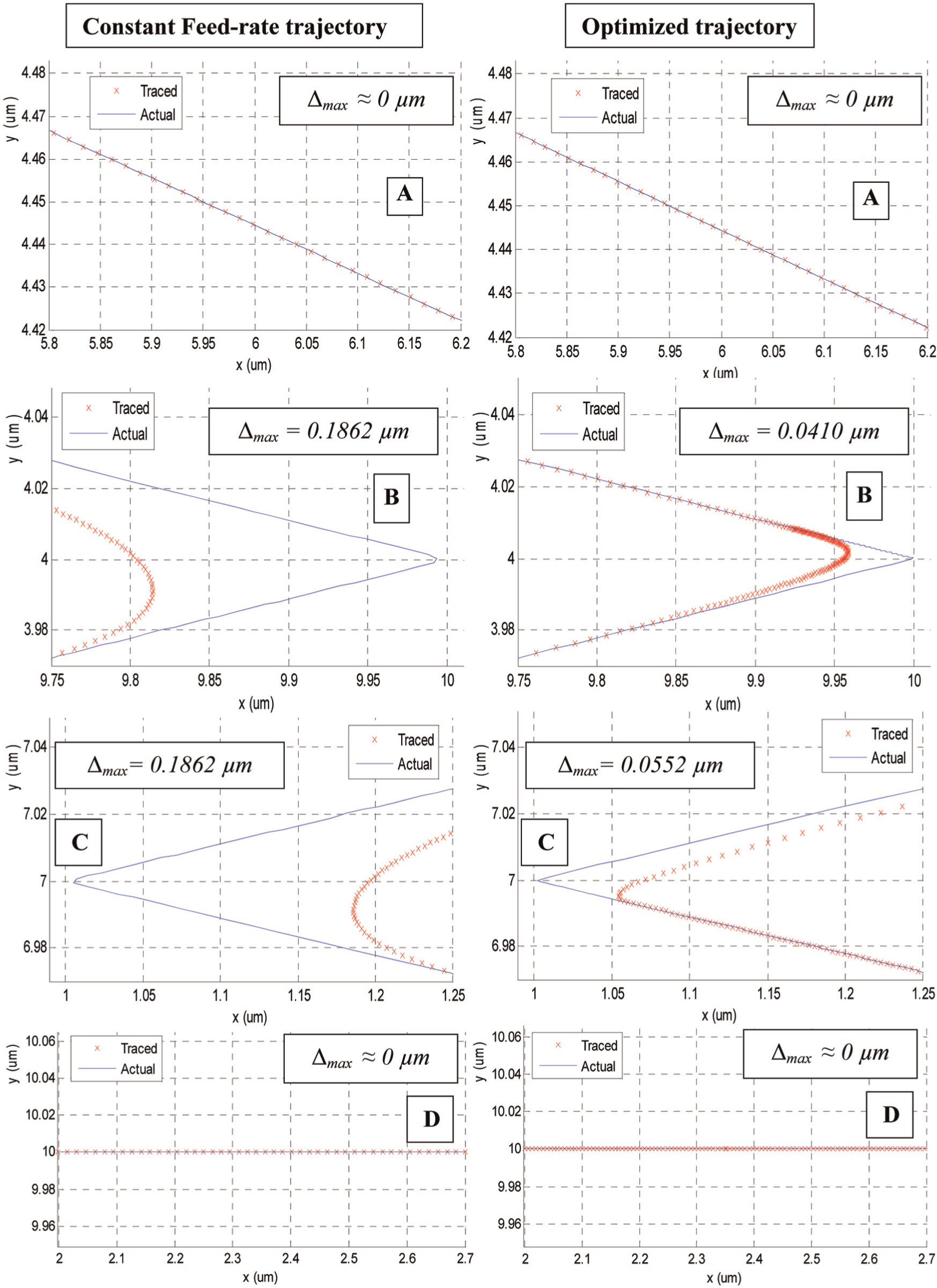
Comparison between optimal trajectory and constant feedrate trajectory subject to actuator constraints at regions A–D on the path of linear trajectory.
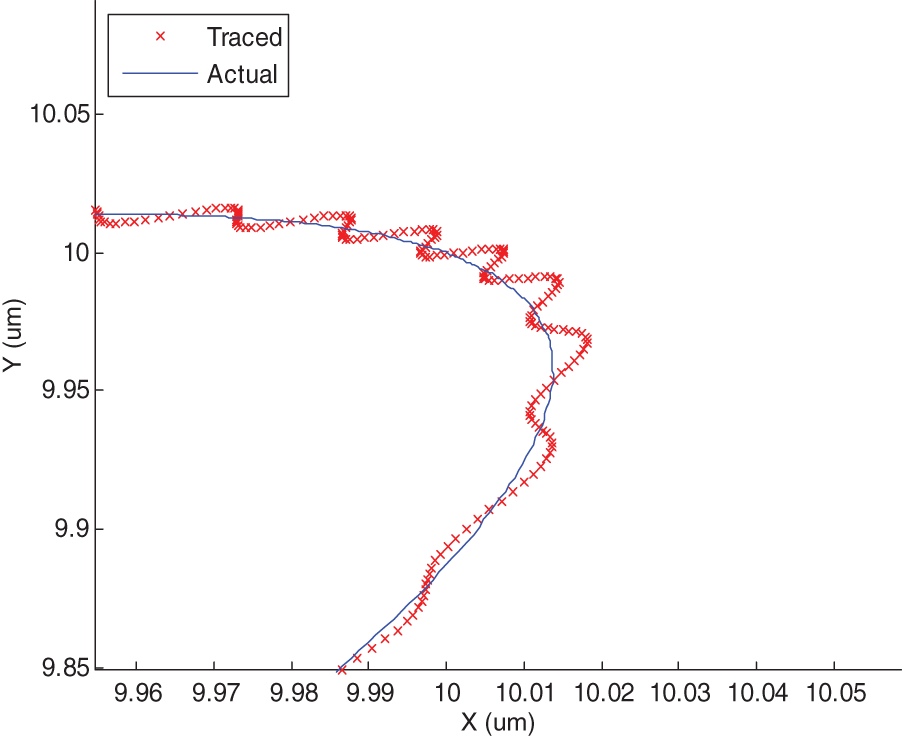
For the airfoil trajectory, the algorithm is subject to all the three constraints developed in section “Modeling constraints from actuator limitations and accuracy requirements.” The contour error constraint was taken to be 0.01 μm and input command bandwidth is limited to 300 Hz. Figure 10 illustrates the application of the feedrate optimization algorithm to the trajectory shown in Figure 7(b). In Figure 10(a), symbols are used to denote the particular constraint that is binding at each point on the trajectory. The contouring results are compared with the constant feedrate trajectory, which is the common industrial practice. To provide a fair comparison, we have adjusted the velocity in the constant speed trajectory such that the actual execution time between the optimized trajectory and constant speed trajectory is same. In Figure 10, the tight contouring error constraint is represented in the performance envelopes and the trajectory by the “Δ” symbol (green); they dominate in many regions of the trajectory for achieving better results. The results of contouring are shown in Figure 11, where the optimal trajectory is compared to the constant feedrate trajectory. The graphs show the improvement in accuracy to within the set error limits. Hence, the user can now be rest assured of the worst-case accuracy in the contouring output, which is absent in commercially available machines.
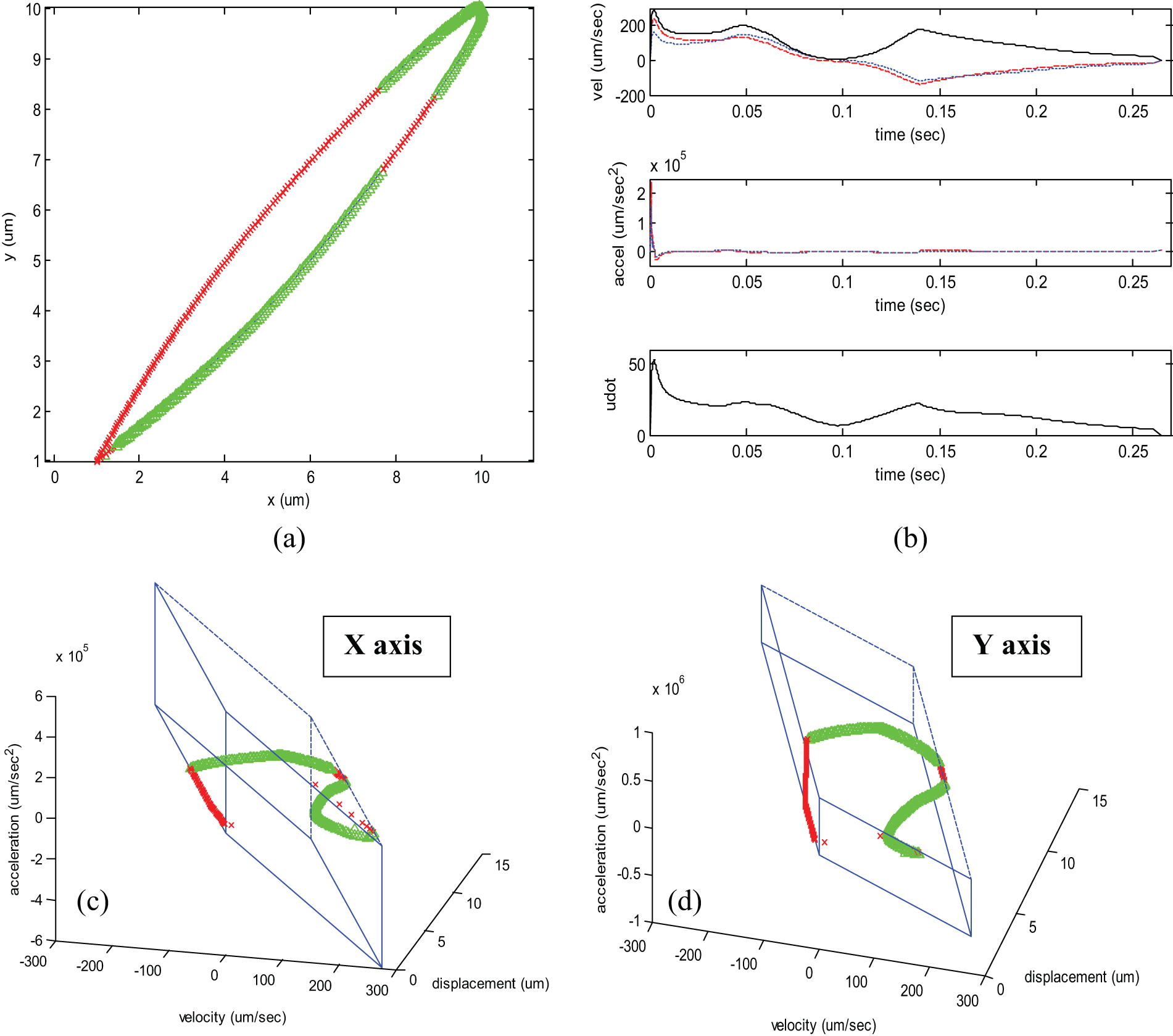
Optimal velocity scheduling with actuator, frequency and contour error constraint; (a) actuator (x, red), frequency (o) and contour error (Δ) constraints are satisfied at all points on the trajectory with one of them being satisfied with strict tolerance; (b) velocity, acceleration and parametric velocity profiles (solid line is tangential, dashed is x-axis and dotted is y-axis) and (c, d) performance envelope for each axis showing the strictly satisfied constraints along all the points of displacement.
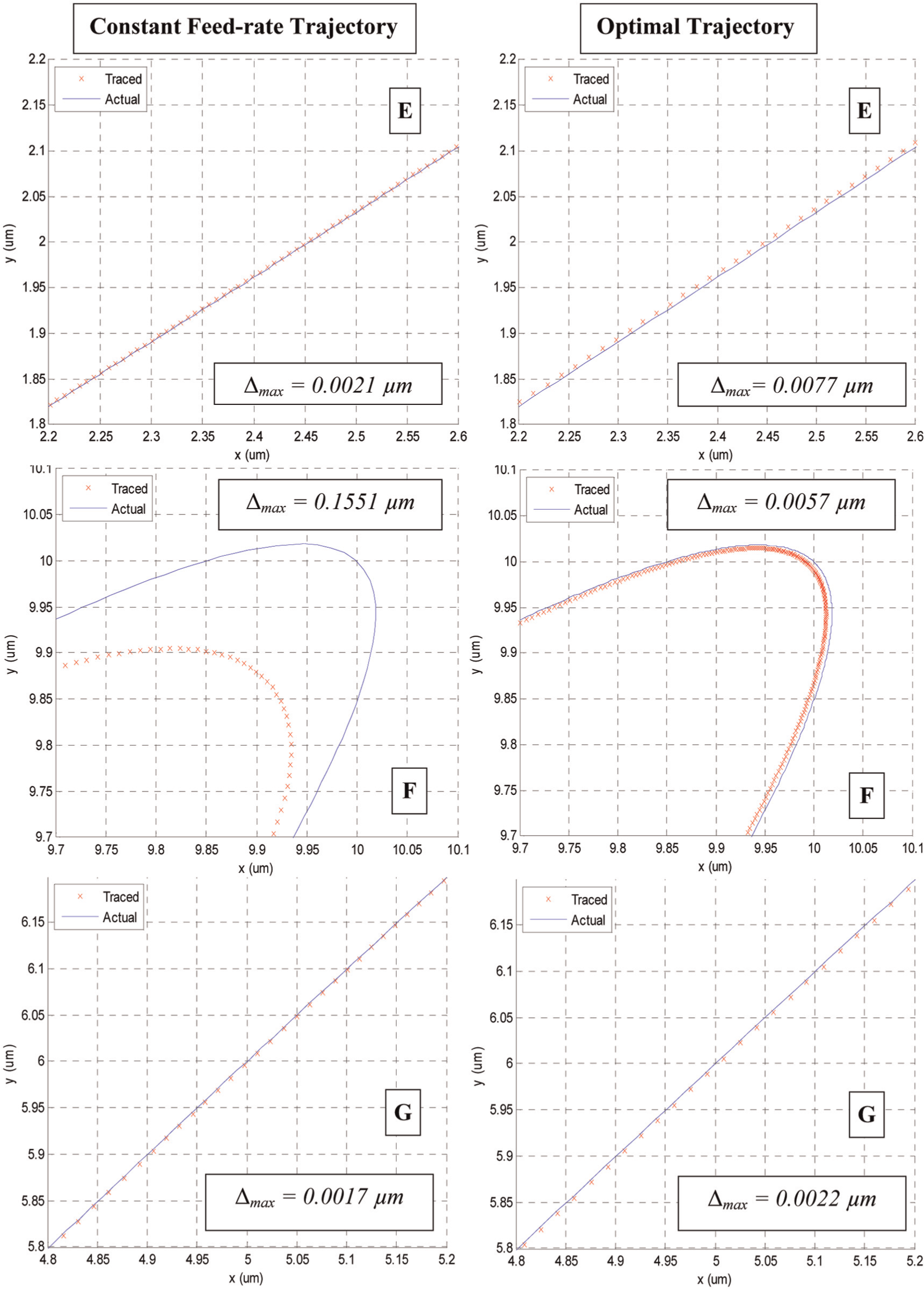
Comparison between constant feedrate spline and optimized trajectory subject to actuator, frequency and contour error constraint in regions E, F and G on the path.
After implementing feedrate optimization and fully considering the capabilities of the system and performance requirements, significant improvement in contour accuracy is achieved. For the zigzag tool path, the contouring accuracy at the sharp corners was improved by 78% and 70%, respectively, for regions B and C, with the error reducing from 0.1862 to 0.0410 μm and 0.0552 μm. For the airfoil tool path, the maximum contour error for the full path has been reduced by 95% from 0.1551 to 0.0057 μm, in comparison to the constant feedrate trajectory.
Conclusion
This article has presented a feedrate optimization approach to achieve high-performance contouring in nanomanufacturing systems by characterizing the capabilities of a nanomanufacturing system and utilizing such capabilities to achieve the required contouring accuracy. This work successfully developed a framework for abstracting the capabilities of a piezo-actuated nanopositioning systems and a methodology for using these capabilities to generate an optimal trajectory for a particular tool path on a given nanopositioning system while satisfying all the process-related requirements. Several dynamic capabilities of a typical piezoelectric actuator-driven nanopositioning system were identified and modeled as constraints to drive the optimization problem, including coupled displacement, velocity and acceleration capabilities of each individual axis, input command bandwidth constraint and contouring error constraint. These developed constraints were incorporated in a computationally efficient bi-directional scan feedrate optimization algorithm to generate a minimum time feedrate profile for any given tool path. The zigzag and cubic spline airfoil trajectories were used as test trajectories to demonstrate the significant improvements in tracking time and contouring accuracy that were realized from the above-mentioned approach. After this optimization strategy is applied, contouring error was reduced significantly (up to 90%), compared with the conventional trajectories executing in the same amount of time.
Footnotes
Declaration of conflicting interests
The authors declare that there is no conflict of interest.
Funding
This research received no specific grant from any funding agency in the public, commercial or not-for-profit sectors.