A step-by-step approach for modelling complex systems with Partial Least Squares

Abstract

The role of statistical analysis to improve business decisions is uniquely appropriate for engineers to champion. As systems engineering has become more widespread, engineers are developing models with a holistic view. These models are complex, requiring both theory and data to construct them. Partial Least Squares is introduced as a modelling technique that bridges the gap between engineering and business. Each of the three modes of Partial Least Squares Regression (Mode A, Mode B and Mode C analyses) is discussed with applications of each demonstrated with two case studies from industry.

Introduction to current trends in modelling

An approximate answer to the right question is worth a great deal more than a precise answer to the wrong question. (John Tukey, 1915–2000, American statistician)

The ability to construct a valid model of a complex system lies at the very heart of science, medicine, engineering and econometrics. ¹ There is a trend in engineering, as is commonly seen in medicine, to adopt a more holistic view of systems. Whereas behaviour at the basic component level may be modelled in deterministic ways by applying generalised laws, as they are integrated into more complex systems, their contribution to the behaviour of the system, and vice versa, becomes less well understood.

Behaviour of the system becomes increasingly less deterministic and more chaotic, as a result of complex interactions and external influences. ² The modelling of such systems therefore becomes less theory but more data driven, and possibly a combination of both. A generic system’s model is shown in Figure 1. It reflects the concept that the behaviour of a system can include many different measures, internally and in terms of inputs and outputs. Measures may be process, environmental, material or human related.^3,4

Figure 1.

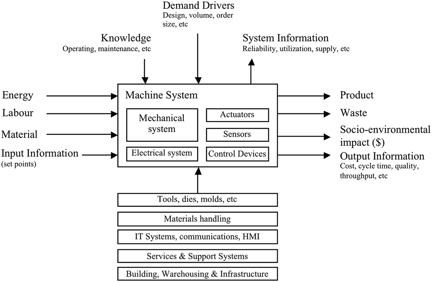
Machine system abstract.

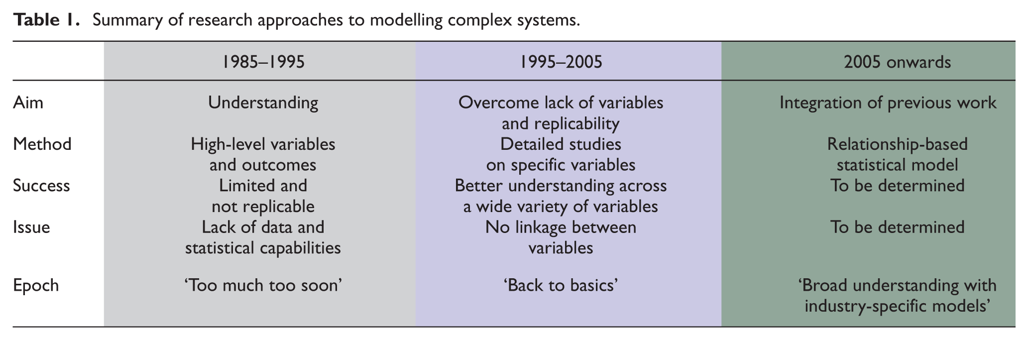
Research on modelling complex systems has evolved over the last three decades: starting from a position where the aims were perhaps overambitious and models were accordingly oversimplified (typically the 1980/1990s), to a philosophy of ‘back-to-basics’ that resulted in more knowledge about specific variables within smaller subsystems (mid 1990s to mid 2000s) and to the present, where the focus is now on integrating better knowledge at the subsystem level into more complex and higher level, and increasingly industry-specific, systems and models. Table 1 summarises these progressions. Complex models are increasingly contingent on specific circumstances, rather than generic factors. The modelling philosophy and approach may be generic (repeatable), but the resulting model is less likely to be so.

Table 1.

Summary of research approaches to modelling complex systems.

	1985–1995	1995–2005	2005 onwards
Aim	Understanding	Overcome lack of variables and replicability	Integration of previous work
Method	High-level variables and outcomes	Detailed studies on specific variables	Relationship-based statistical model
Success	Limited and not replicable	Better understanding across a wide variety of variables	To be determined
Issue	Lack of data and statistical capabilities	No linkage between variables	To be determined
Epoch	‘Too much too soon’	‘Back to basics’	‘Broad understanding with industry-specific models’

Many researchers and industry practitioners start out with the aim and desire to create a ‘super-model’, one that will address all of the perceived issues of the real system and extract the maximum meaning from the data set. ⁵ The presence of large data sets should in theory enable substantial information and insight to be gathered and used to better manage the system or process. However, data in its raw form are rarely useful or representative of the true underlying behaviour or state of the system. ⁶ More often than not, there exists a particular aspect to the behaviour of a variable, a key feature, which characterises the behaviour and state. Identifying and extracting such features normally requires extensive analysis at the detailed component or subsystem level, before it can be used at the next level in the model hierarchy. It is usually better to split a large issue or model into smaller sub-models and integrate these further down the track.

Purpose of the model

Perhaps the most important issue is the purpose of the model, particularly the extent to which the model is to be used for forward prediction, given a current state and a set of future inputs, or for backward explanation, given a current state and current inputs, the latter with the aim of identifying those variables or measures that are causally related and may be manipulated or improved. ⁷ In some applications, the only aim is to predict the future, without extracting any further meaning in relation to what may or may not cause system behaviour.

In engineering, improving the existing system or the next generation of systems is of equal or greater importance than simply understanding system behaviour. Most models therefore rely on identifying those key variables or features that have the greatest predictive power on the one hand and, from a causal point of view, have the greatest bearing on the behaviour or state of the system on the other hand. The initial modelling approach therefore can be described as ‘top-down’–‘bottom-up’. The focus on a particular aspect of system behaviour is usually defined from the top-down, whereas the measures, features or variables are identified and quantified from the bottom-up. ‘Bottom-up’ does not necessarily imply that the measure must be from the lowest order in the hierarchy. In a practical sense, it means that in most cases, it starts as a measure immediately below the ‘top-down’ or ‘effect’ variable. As more detail or understanding is called for, this process is repeated down, until the behaviour of key components or subsystems can be sufficiently accurately characterised in terms of basic formative measures, or in the case of human-centred systems and processes, basic formative questions.

Model characterisation

Characterising and modelling complex systems start by identifying performance objectives, in other words, those constructs or parameters that the study would want to optimise. Depending on the nature of the system, these can vary considerably. In the case of a machine, for example, these may be availability, output and quality, the traditional measures for overall equipment effectiveness (OEE). For a business process, such as research and development, these could include deliverables such as quality of output, milestones achieved and percentage cost overruns.

The next step would be to identify variables and measures that may influence these higher level constructs. This can be a very detailed and time-consuming exercise and usually draws upon a variety of analysis techniques ranging from traditional cause–effect analysis to more detailed interaction charts, affinity diagrams, matrix diagrams, issue analyses and so on. The outcome of this phase will be a data set of key variables (measures) that may affect the behaviour of the system or process.

The extent to which these data can be used in a model depends on the nature and complexity of the system and the level of information contained within each variable or measure. To clarify this, if the system is a business process and the variables or measures are answers to questions on a carefully designed questionnaire, then there would be little additional information for each variable other than the answers recorded, usually on an ordinal scale. On the other hand, if the system involves a machine or industrial process, and key process variables are logged, then the data contain substantially more information than just the stream of numbers communicated by the sensors. In this case, the data set is usually not suitable for immediate modelling and an additional analysis phase commences. This phase may be termed a pre-analysis phase ⁶ where the objective is to create a consistent, coherent and material observation set for statistical or other analysis. Raw data may need to be time-stamped, cleaned, filtered, transformed, key features extracted and time synchronised.

Data types

Data may be classified in a number of different ways including the following:

• Data type

• Integer – coding of categorical data, units produced and number of failures in a given period of time.

• Discrete – data that are counted. This can be acquired at specified points in time, for example, questionnaire data obtained at monthly intervals, process measure logged every 1 s.

• Continuous data – data that are measured. This is usually on an interval or ratio scale.

Data scale

Nominal – qualitative or categorical data, where categorical labels are represented by integer numbers. Examples include type of product produced, day of week, shift team, maintenance team and so on.

Ordinal – quantitative non-parametric data. Typically responses to a questionnaire that are scaled say 1–10, where the order of the response is important but where the differences are not.

Interval – where the unit of scale interval is relevant but the origin of the scale is arbitrary (typically degree Celsius and Fahrenheit). Time-stamped data also fall in this category (yyyymmddhhmmss).

Ratio scale – most physical measures such as length, mass, pressure and time duration.

Data source or origin

Man – questionnaire data, attribute data such as skills and training and psychological data including motivation.

Machine – critical process variables, machine state, utilisation, age, condition, reliability, capability and so on.

Material – material attributes such as type, surface conditions, strength and hardness.

Method – operating set points and maintenance tasks.

The nature of complex systems

Complex systems can usually be characterised by multiple inputs and outputs, multiple internal variables and interactions, and indeed multiple subsystems and interactions between subsystems. Examples of this include engineering designs such as machinery, electrical equipment and most industrial processes. It is the task of the design engineer or scientist to identify the minimum set of critical design and manufacturing parameters that individually and collectively achieve the design or functional requirements.

Methodologies such as quality function deployment and axiomatic design attempt to achieve exactly this, the progressive translation of higher level specifications into more detailed and lower level ones, until an unambiguous and definitive set of design variables can be established. In the event that a design exists and needs to be improved, which is often encountered in process and continuous improvement, the methodology of process identification, characterisation and modelling attempts to achieve the same outcome, that is, a set of critical process variables and measures that describe and predict the performance of the system, with the aim of manipulating these variables to improve performance.

If the design is new, or the system not well understood, then these tasks become more difficult. There may be hundreds or more variables and interactions. System behaviour may be as much a function of physical design as it is of the operating environment and human intervention. If the design is novel, there may be a lack of data, and the analysis may rely heavily on expert opinion and perhaps simulated data. On the other hand, for an established system, there may be an abundance of data, at the system and subsystem levels and at machining, processing, operating and maintenance levels. More often than not, it is important to consider all data, initially, and identify those variables or key features that account for most of the system behaviour that the study is focused on. The initial data set may be large, but once key features are extracted, ordered, aligned and matched according to the interactions to be tested and quantified, the resulting observation set is substantially reduced. It is also important to identify different system states, and that the transition from one state to another is not necessarily a continuous one. The overall or global behaviour of the system is a collection of local states, and different characterisation or transformation models may dominate behaviour around different local states.

It is important to test system behaviour both at the system and subsystem levels. The aim is first to identify those measures that are critical to defining behaviour at the subsystem level, and this is primarily an analysis with the aim of reducing data. The second aim of the analysis is to model and analyse higher level interactions in order to improve the behaviour of key system parameters. The analysis then focuses on modelling and improving the behaviour of low-level design or performance variables at the subsystem level in order to improve performance of the next level in the hierarchy and ultimately the system as a whole.

Partial Least Squares

Partial Least Squares Structural Equation Modelling (PLS-SEM, also known as Partial Least Squares Path Modelling (PLS-PM)) is a technique that lends itself particularly well to initial exploratory analysis in order to establish and rank order key indicators or measures (based on construct weightings, correlations or both) and to determine what avenues to pursue in order to gain more insight and understanding. From a purely inductive point of view, the aim is to design a structure, and to identify those constructs and indicators that possess the greatest predictive ability, regardless of any causal relationship. From a deductive perspective, the aim is to confirm a causal or nomological network that reflects, to a lesser or greater degree, the hypothesised underlying general or covering theories, combined with empirical measures that support the constructs. Combining the two analysis techniques, in a forward predictive and backward explanatory mode, may yield the best of both worlds, namely, the identification of a set of ‘key’ constructs that allow for prediction and prognosis, coupled with maximised information gain at the formative measure level in order to improve the underlying behaviour of the system itself. PLS is based on the assumption of linearity of the data set. If the data are non-linear, the data can either be transformed or an alternative analysis method is required.

Defining the research problem

All modelling begins with a broad understanding of the domain area. Data have been collected either through data acquisition systems or through individual sources (questionnaire data). As PLS has a number of applications and two distinct assumptions of variance for indicators, it is critical the researcher understands how they expect the data for each of the indicators to change with respect to that of the other indicators. In terms of PLS, a clear distinction needs to be made regarding the variance of interest in each part of the model.

For the purpose of reporting and discussing PLS models, variable is referred to as any aspect or item of interest. If data can be collected, then the variable is considered an indicator in a PLS model. Indicators are either formative or reflective. If a variable does not have any data but acts as a grouping attribute, then it is considered a construct. Indicators are linked to constructs to form a component. PLS models often have many components linked together in a non-linear way. A PLS Regression model only has two components, whereas PLS-PM has three or more components linked together.

The expectation regarding variance is based on whether indicators are formative or reflective. Formative indicators are those indicators that are expected to form or cause the concept to exist in the way it does. Formative indicators are items that all tap into the underlying concept (construct), they are specific and try to isolate only part of the concept. There is no reason any of these indicators should correlate with each other. Reflective indicators are those indicators that are expected to reflect the construct to exist in the way it does. Reflective indicators are items that are viewed as being effected by the same underlying concept (or construct); if the construct was to move in one direction, it is expected that these would move in the same direction. Reflective indicators should all correlate highly with each other.

In an engineering process line where the aim is to increase production, formative indicators might include the pressure within a specific tube, the deviation from the mean of a specific part, the temperature of the curing oven and the duration of the cooling process. Reflective indicators might include the line speed and OEE. In a business setting where the aim is to improve leadership within the company, formative indicators might include the regularity of communication, the quality of the communication, timeliness of the communication and communication regarding your specific project. Reflective indicators might include the overall communication and communication to your department.

In each of these examples, it was clear that the reflective indictors must have a considerable amount in common, that is, their shared variance is important. There is no expectation that in the examples above that the formative indicators should have much in common. An increase in tube pressure should not necessarily increase the temperature in the curing oven. If line speed increases, we would expect OEE to increase as well. When determining which indicator makes the most important contribution to prediction, all the variance must be included in the analysis.

Unlike its far more well-known statistical cousin Covariance-Based Structural Equation Modelling (CB-SEM), PLS is able to handle both formative and reflective indicators. This allows for far greater flexibility, as PLS can be used as a data reduction technique (PLS Regression) to identify the most critical variables and for final analysis (PLS-SEM) to establish direct, indirect, moderating and mediating effects. The purpose of PLS is therefore twofold. First, it serves as a data reduction technique to identify a reduced set of measures that either predict or are causally related to behaviour (or both). Second, PLS serves to model more complex interactions – direct, indirect, moderating and mediating – between different behaviour constructs at the subsystem level and subsequently between subsystem constructs to explain behaviour at the system level. For the purpose of this article, all analyses are conducted using PLS Regression (two-component models).

Shared and all variance

Components that consider only shared variance include indicators where the change in the direction of one indicator would result in change in the direction (but not necessarily magnitude) of other indicators. These indicators are called reflective indicators as they reflect an outcome.

In engineering, examples of shared variance problems include output of a production line (parts per hour). For output of a production line to increase, it would be expected that the speed of line, the speed of the machines and the speed of the operators would all increase if the output were to increase. Other examples in engineering might include cost of a project (as time increases, more staff hours are required, machinery utilisation increases).

In business, examples of shared variance include staff retention rate. For staff retention rate to increase, it would be expected that staff are satisfied with management and staff requests for specialised training and the proportion of early arrivals would all increase. Other examples in business might include technology uptake (staff with more devices tend to have exposure to more technology and have an interest in new technology).

Components that consider only shared variance can of course move in an unfavourable direction. In both of the previous examples, the output of the production line and staff retention rate could both decrease. In this case, it would be expected that the same indicators that increased previously would now decrease. Each of these indicators should trend in the same direction, if this was shown not to be the case, then the model would need to be reconsidered and the assumptions underlying the model verified.

Models that consider all variance in the indicators are similar to multiple linear regression. Indicators need not change in the same direction (nor magnitude) as the aim is to achieve the highest possible combination of all the variance being accounted for. These indicators are also called formative indicators as they form the basis of the observed outcome.

In engineering, examples of indicators where all the variance is included are processes with multiple inputs to a product (chemicals, metals, temperature, time) with one specific measure (weight, size, surface finish). In business, examples of indicators where all the variance is included are processes from separate departments (finance, human resources, R&D) with one specific measure (revenue, profit, price/earnings (P/E) ratio).

PLS modes A, B and C

PLS has two types of prediction, using shared variance (reflective indicators) or all variance (formative indicators). PLS Regression where the indicators are reflective can be considered analogous to Factor Analysis. Whereas PLS Regression where the indicators are formative can be considered analogous to Principal Component Analysis. Both Principal Component Analysis and Factor Analysis attempt to summarise patterns of correlations among observed variables to a smaller subset of either components or factors. Principal Component Analysis accounts for all of the observed variance and is therefore empirical in its nature, whereas Factor Analysis only analyses shared variance.

Factor Analysis attempts to eliminate variance due to error and variance that is unique to each variable. Tabachnick and Fidell ⁸ provide an excellent summary of the differences between Factor Analysis and Principal Component Analysis. Factors are thought to ‘cause’ the variables, the underlying construct is what produces scores on the variable. Consider the score on any variable, where the components are simply aggregates of correlated variables. Considering Factor Analysis in terms of Linear Regression, the factors are the independent variables (IVs), which produce the dependent variable (DV). Considering Principal Component Analysis in terms of Linear Regression, the variables are the IVs that produce the component the DV.

Using an example developed based on hypothetical data from the review of one of the author’s doctoral thesis, an example of PLS Regression using three different modes of analysis is shown. Mode A analysis (Figure 2) is a PLS Regression model where both constructs have only reflective indicators. Mode B analysis (Figure 3) is a PLS Regression model where both constructs have only formative indicators. Mode C analysis (Figure 4) is a PLS Regression model where one construct has only formative indicators and the other construct has only reflective indicators.

Figure 2.

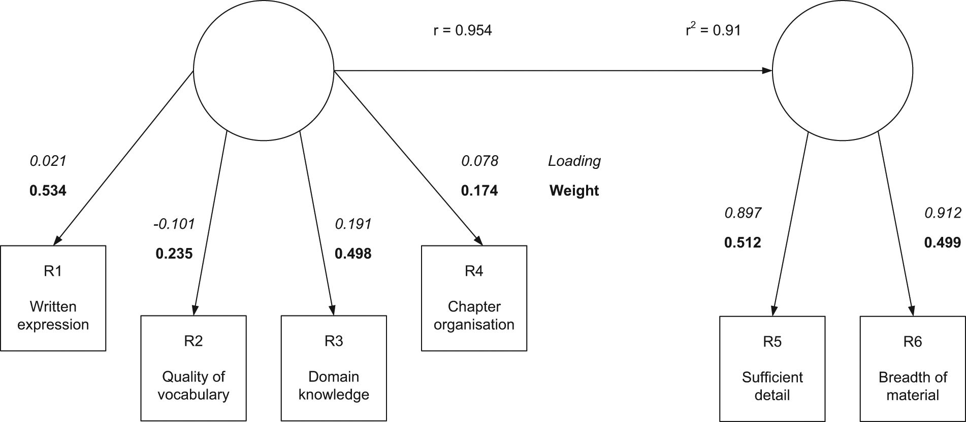
PLS Regression using Mode A analysis.

Figure 3.

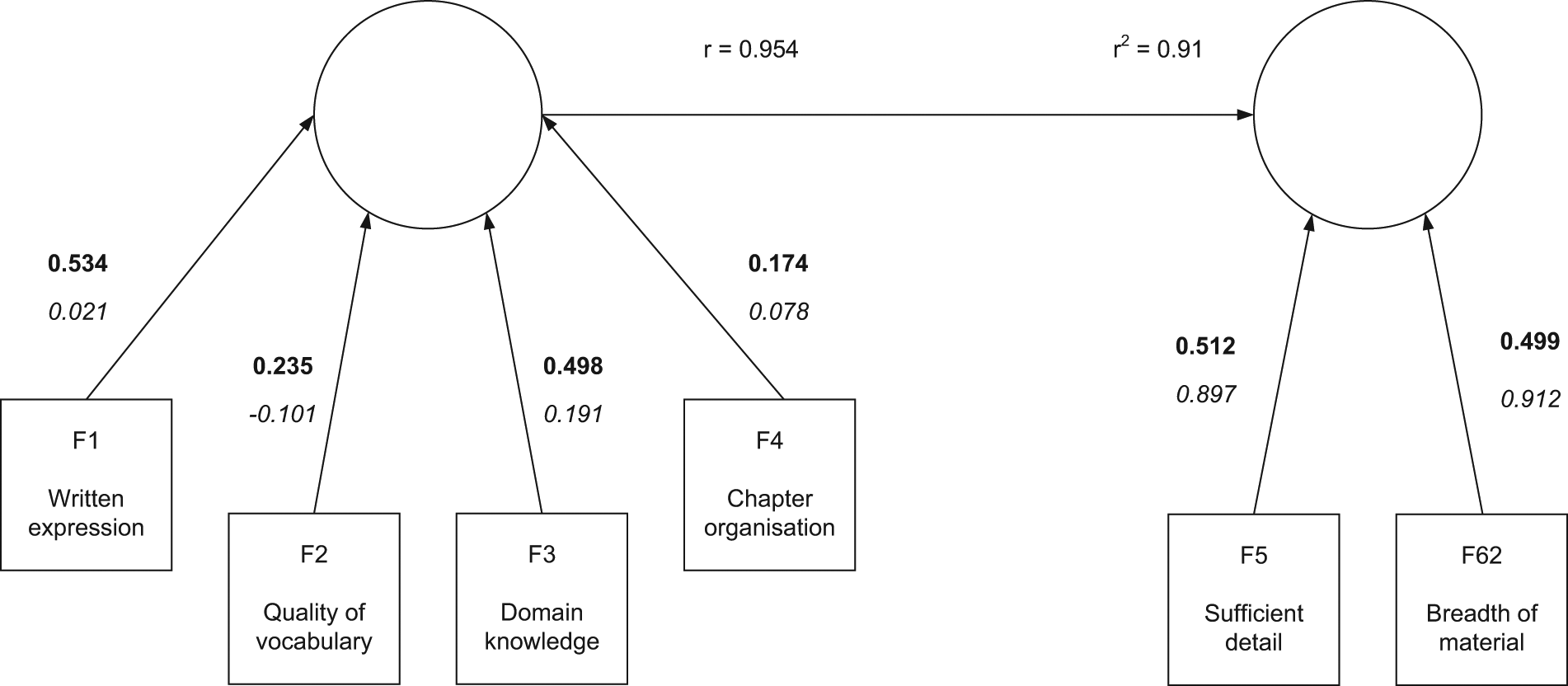
PLS Regression using Mode B analysis.

Figure 4.

PLS Regression using Mode C analysis.

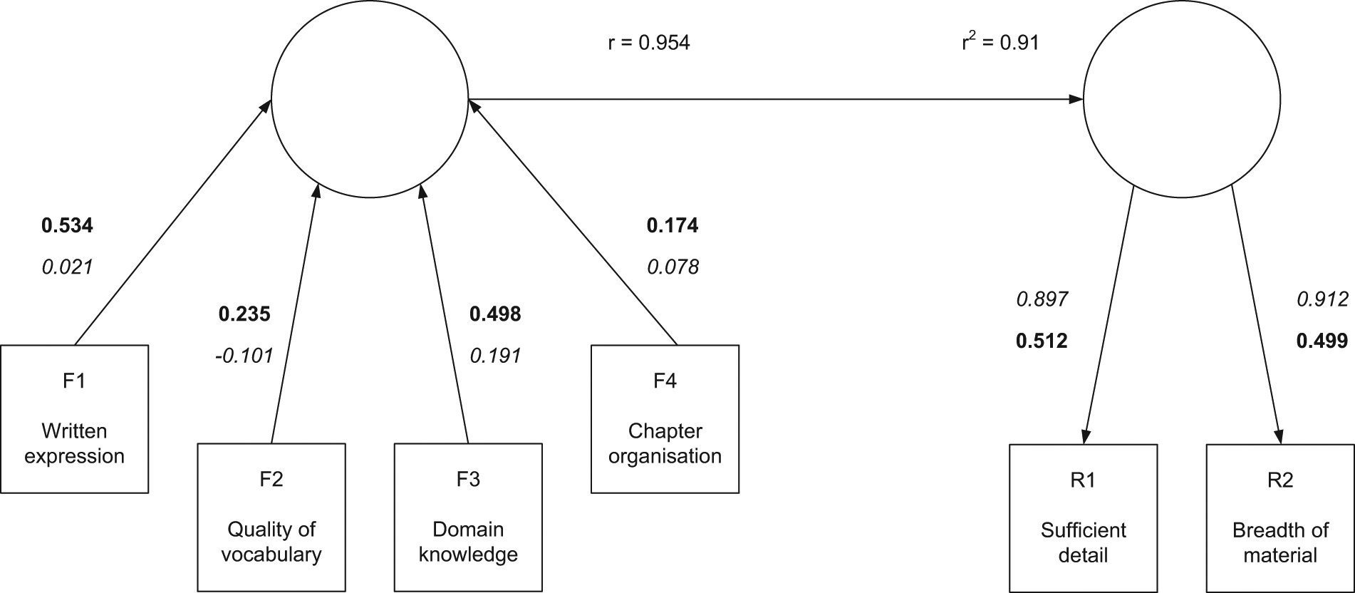
Modes A, B and C analyses are shown as follows with interpretation. Figure 2 shows Mode A analysis as both components have reflective indicators. On the left-hand side, there are four indicators each describing different measures of the doctoral thesis. The hypothetical example was based on an 11-point Likert scale centred on zero, where a higher score indicates a greater level of overall satisfaction. Running PLS Regression in Mode A analysis, we can see that of the four indicators, two have a reasonably high weight (R1: 0.534 and R3: 0.498) and other two less so (R2: 0.235 and R4: 0.174). All four have a low loading (R1: 0.021, R2: −0.101, R3: 0.191, R4: 0.078) which suggests that the indicators are not correlated with each other. Weights are in bold and always closest to the arrow head in PLS model; loadings are in italics, furthest away from the arrow head. Based on this, we could presume that ‘written expression’ captures part of ‘quality of vocabulary’ and that ‘domain knowledge’ captures ‘chapter organisation’. Both of these conclusions seem reasonable. It is worth noting that the reverse situation would have been equally plausible. The conclusion we draw from the Mode A analysis is that the component on the left-hand side is a very good predictor of the component on the right-hand side. These two reflective components are quite similar and there would be the potential to remove one from the final model.

Taking the same data from the review of the doctoral thesis, this can now be analysed with PLS Regression in Mode B analysis. Mode B analysis would be used where we believe there to be no underlying change in direction between each of the indicators. Whereas in Mode A analysis, PLS Regression was attempting to find shared variance across the indicators; in Mode B analysis, now all of the variance is being considered. In Figure 3, the same four indicators (now F1 – 4, as opposed to R1 – 4) are now being used to see how they form predictors for the formative indicators F5 and F6. In this analysis, once again F1 and F3 are stronger predictors, than F2 and F4. When considering all the variance, the indicators F2 and F4 now have a greater importance than in Mode A analysis.

Combining formative components and reflective components in PLS Regression results in Mode C analysis. Mode C analysis is a predictive model using the formative indicators F1–F4 to predict R1 and R2. In this model, the four formative indicators predict 95% of the total variance in the two reflective indicators. The weights suggest that F1 and F3 are the indicators producing most of this prediction. Of the reflective indicators (which are looking at shared variance), both have a very high loading (correlation R1: 0.897 and R2: 0.912) with each other relative to the formative indicators. This suggests how reviewers felt about the level of detail strongly correlated with the breadth of material in the doctoral thesis.

Having now presented a summary of the three main modes of PLS Regression, an approach for using these is presented in the course of analysis.

• Identify those measures formative and reflective best represent the system and the subsystem. Start at that point where the most meaning (result of cause–effect analysis or prior knowledge) is likely to be found.

• Separate the measures into formative and reflective indicators. This may not always be obvious, except that causal variables can usually be considered formative (when they have data).

• Run Modes A, B and C analyses to test the indicators and select the most appropriate one on the basis of (1) their contribution to total variance and (2) their share of shared variance.

• When the model becomes more complex, either by adding more components or expanding the model in a hierarchical sense (upwards at the system level or downwards by including additional subsystems), the PLS analysis mode becomes Mode C analysis by default.

When looking at constructs in isolation, the overall explained total variance (R²) is not always as high as would be ideal. This is understandable because there are likely other constructs that have not been modelled yet. This is not a reason to discount the analysis because at this stage, the focus is still on reducing data. As the PLS constructs are assembled into a larger PLS-PM, more of the variance will be explained.

Application of PLS to improving industrial machinery

The behaviour of industrial machinery is often expressed as OEE, a function of performance, reliability and quality, as well as various cost-related measures. These parameters in turn are usually supported by indicators such as, in the case of reliability, mean time between failure (MTBF), downtime, lost production and process availability. The relationship between these is straightforward and easy to understand. The reasons or causes are less clear and there are likely many variables or measures, sometimes co-related, more often not. In constructing models, it is important to combine theoretical knowledge (e.g. physical relationships) with latent knowledge held by process operators, engineers and maintainers. An example of this is shown in Figure 5.

Figure 5.

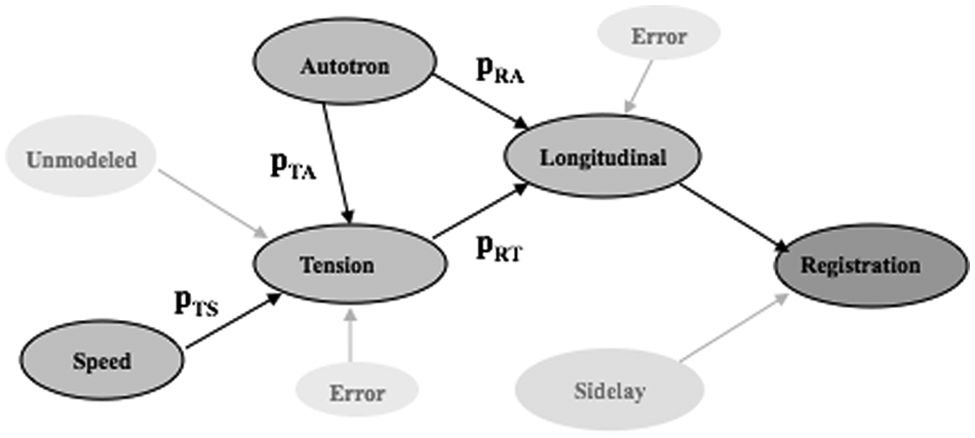
Causal model representing errors on a printing press. ⁹

This causal model of registration error on a printing press reflects physical laws in the sense that tension variations in the material between printing stages are a direct cause of registration error and that variations in the speed of the press are in turn a direct cause of tension variations. Not as obvious is the effect from a measure called ‘Autotron’. An autotron is an actuator that advances or retards print material between two consecutive print cylinders. Its behaviour is automatically controlled by a proportional–integral–derivative (PID) controller with registration error detected by a vision system as the feedback signal. The duration of the advance/retard action is proportional to the size of the error. It has a direct effect on registration error, but also an indirect effect. This understanding was based on latent knowledge from process experts. This particular model was used to predict quality problems and subsequently used to successfully improve the process. ⁹

This leads to the next key issue, which is that aside from the fact that there are many, hundreds or more, variables that can characterise a complex system, these variables can take on very different attributes and characteristics. Most low-level component-related variables tend to be continuous physical variables, such as temperature, vibration or pressure. Higher level parameters, such as reliability, can be exact or censored, continuous or discrete-event data represented as failure modes, condition or inspection data. Performance and quality data can include millisecond process data as well as data collected for a particular shift, as well as weekly or monthly trend results. Processes involving human activities are a rich source of data and information and may include the level of training, skill and motivation. These data are often expressed on a nominal scale, say from 0 to 10. To further complicate the analysis, the underlying process behaviour may have elements that are deterministic, stochastic, time-(in)variant, linear and non-linear, monotonic or non-monotonic.

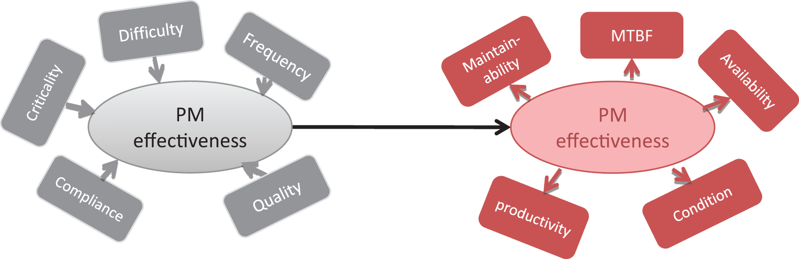
How a machine is maintained may have a profound impact on how the system behaves and degrades over time. Figure 6 shows an example that deals with a formative component called ‘PM effectiveness’, which may be interpreted as the extent to which a preventive maintenance task successfully improves reliability. It is hypothesised in this case that the five formative measures collectively determine the effectiveness of the PM. The five are the quality of the PM (a subjective but important assessment), its frequency of planned execution, schedule compliance (perhaps more a mediating rather than direct factor), the criticality of the PM (in terms of aligning with a major potential failure mode or mechanism) and its level of difficulty.

Figure 6.

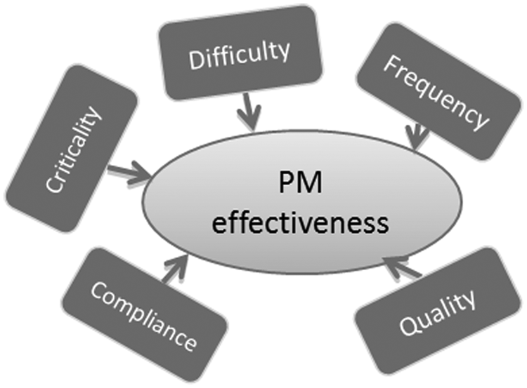
A component representing PM effectiveness formed by a number of formative indicators.

The question may be asked, which of these measures are the most important for improving the effectiveness of preventive maintenance? Analysing the data and structure in Figure 6 is insufficient, and meaningless, in the absence of data that describe the construct itself. This question can only be answered when a reflective counterpart is introduced, as shown in Figure 7. In this case, PM effectiveness is represented as a reflective component, and the reflective indicators are MTBF, failure frequency, availability, maintainability (a reduction in breakdown costs) and machine condition. These indicators are, with the exception of condition, reasonably objective and easily quantified. All reflective indicators must strongly correlate with the construct, to be considered representative of the construct itself.

Figure 7.

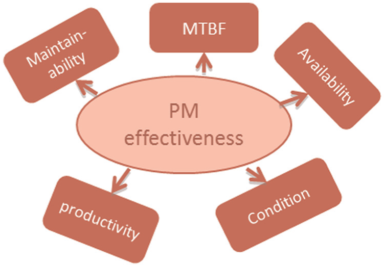
A component representing PM effectiveness formed by a number of reflective indicators.

Based on available data and a (causal) model or path structure, the aim is to determine the predictive ability of the formative component onto the reflective component and its indicators, as shown in Figure 8. A number of important outcomes are achieved here. PM effectiveness is no longer a subjective measure; it is now closely linked with its reflective counterpart that in turn is based on a set of indicators. The formative indicators can now be directly regressed onto the reflective indicators and used for prediction as well as causal analysis. Finally, this analysis points to those formative indicators that play the greatest role in predicting the reflective indicators and those that are, nomologically, the most likely candidates for improvement in an engineering sense. The integrity and quality of this model are reflected by the R² between the two components and depend on the availability and quality of data, on the selection of and information contained within the indicators and on the design of the structural model itself. In this simple model, only two components were considered. There may be many more. In this sense, designing a PLS-PM (as opposed to a PLS Regression model) is as much an art as it is lengthy exercise in exploratory and confirmatory analysis.

Figure 8.

PLS Regression model (Mode C analysis) containing a formative and reflective component.

This technique can also be applied in a hierarchical sense, where a number of such constructs become the formative measures for the next higher level construct, and so on. The philosophy is then one of starting with relatively simple component and expanding the analysis in both an up and down and sideways direction as the model and its underlying process are better understood and more knowledge is required or desired. This is consistent with the evolution of modelling described earlier. It may be that certain variables and interactions are better modelled using alternative techniques from either the statistical (e.g. Bayesian), mathematical (e.g. control theory, state-space analysis) or artificial intelligence (e.g. neural networks) disciplines. Those are decisions that can be made at any stage in the analysis and model design.

Since the analysis focuses on the most critical measures and relationships, it makes the process itself an efficient one. It also means that it lends itself to adding value in the short, medium and long term and this is critical in delivering continuous improvement. As with any analysis, decision support or software implementation, the level of detail and sophistication and hence investment must ultimately be related to the potential benefits obtained from improved information, knowledge and understanding, and this is naturally very much application driven.

A case study using PLS Regression

To illustrate the use of PLS Regression in industry, a case study of a medical supply manufacturer is discussed. One of the products made by the company is an intravenous bag. This product has been in production for more than 13 years. The production line consists of 22 workstations which are predominately operated by pneumatic cylinders. In total, there are more than 600 pneumatic cylinders operated via a logic sequence predefined by the machine’s programmable logical controller (PLC). The performance of the machine is recorded continuously by the on-board supervisory control and data acquisition (SCADA) system. One major issue that the production line has encountered for many years is the relatively poor OEE.

The production line is a complex operation because of the large number of dynamic components. It would be impossible to model the behaviour of such machine mathematically within any reasonable timeframe. The nature of the data is also very complex. The data used can be divided into two categories: hard data and soft data. Hard data refer to numerical values (e.g. product rate and yield, set points, amount of reject and cycle time). Hard data are usually less subjective to human biasness given that the data collection plan is well established, controlled and implemented. On the other hand, soft data often involve certain degree of subjectiveness (e.g. questionnaire responses from engineers and operators). In traditional data analysis, soft data are often overlooked as there is no standard method to build relationships between the hard data and soft data. ¹⁰ In addition, there is also considerable tactile knowledge of the machine that is not being captured such as operator input. In the production line previously described where the machine is highly customised, and additional consideration is the constant upgrade of subsystems, it is virtually impossible to extract useful information from the original design specifications. It is believed that by neglecting soft data, important knowledge and characteristics of the machine will be unexplored. For a standard shift of 8 h, some of the data are collected more than once per shift such as air pressure. Some of the data are collected exactly once per shift such as total downtime, while some data are collected on an infrequent basis such as maintenance cost.

The initial stage of the analysis involved a review of the currently available data. Basic engineering problem identification techniques such as Pareto analysis and cause–effect analysis were carried out to identify problematic subsystems and areas for possible improvement. By using simple validation methods such as time studies, there are six possible areas that may contribute to the OEE issues, which are given as follows:

• Machinery. There may be a small number of critical pneumatic cylinders and dampers that cause a relatively large number of defected products and machine breakdowns.

• Raw materials. The consistency of the raw material may affect the stability and productivity of the machine.

• Compressed air quality. The quality of the compressed air supplied to the machine may effect the wear rates of the pneumatic cylinders and dampers.

• Preventive maintenance effectiveness. The degree of adequacy of preventive maintenance on critical workstations may effect the remaining useful life of the corresponding critical components.

• Communication. The way responsibility is delegated for various problems with the machine may effect the morale of the team which contributes to the degree of commitment to solve problems.

• Operator consistency. The adequacy of training received by the operators and their corresponding skill levels may affect the time required to diagnose problems.

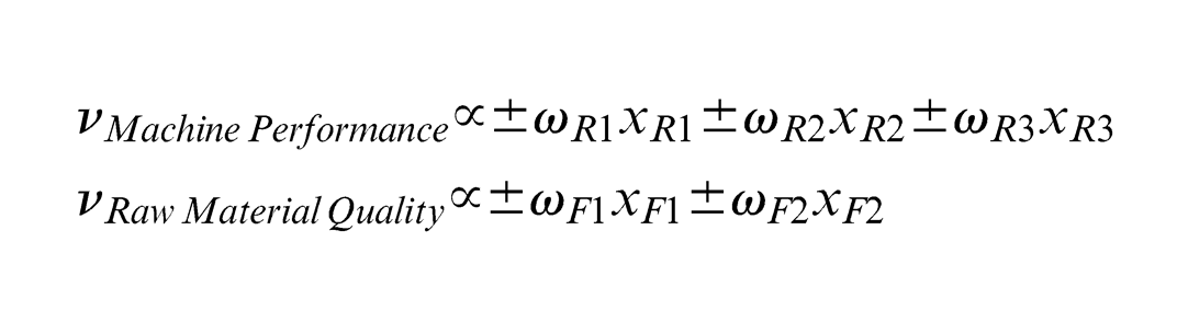
Having identified the main areas that are reducing OEE, the question now becomes ‘Which strategy should the company invest in for the maximum rate of return?’ For the scope of this article, one particular hypothesis was assessed using PLS Regression –‘The relatively low OEE was caused by poor raw material quality’. It was known that one of the raw materials has inconsistent quality due to poor standardisation in the manufacturing stage. Thus, if better manufacturing standardisation was implemented for this raw material, machine performance could be improved. Two formative components were established for this study: ‘Raw Material Quality’ and ‘Machine Performance’. Mode B analysis (canonical correlation analysis) was selected as the starting point to determine the degree of predictive power between these two components. If it can be proven true that one component has high and significant predictive power on the other component, it would then make sense to continue to explore further into this model using Modes A and C analyses. In order to establish formative components, the indicators should be chosen such that they all logically formed the specific concept and they should have minimum multicollinearity among themselves.^11,12 This can be achieved by using well-established engineering formulae and expert knowledge. For instance, ‘Machine Performance’ was formulated by the following indicators: Availability, Productivity and Quality. The multiple of these three parameters give the OEE which is commonly used in engineering as a key performance indicator (KPI) for machine efficiency. The definition of each indicator is outlined as follows:

• Availability (R1) – Total Machine Uptime/Total Shift Time;

• Productivity (R2) – Total Accepted Products/Total Products Produced;

• Quality (R3) – Ideal Machine Cycle Time/Actual Machine Cycle Time.

These three indicators measure the same underlying concept – Machine Performance. In addition, these indicators were composed of independent measurements which could effectively eliminate multicollinearity. There were little performance data available on this raw material. Instead of using hard data to establish the component on raw material quality, expert knowledge was utilised to measure this indicator for this component. This was done by asking two experienced leading hands of the machine to assess and rate this raw material by visual inspection just before the raw material was inserted into the machine. The rating scale used was from 1 to 10, where the rating of 1 represents extremely poor quality and the rating of 10 represents extremely good quality.

The model was based on a data set with 51 data points which corresponded to 51 work shifts. The data were standardised to have mean of zero and variance of one. ¹³ Figures 9 and 10 showed the scatterplot of the indicators for ‘Machine Performance’ and ‘Raw Material Quality’.

Figure 9.

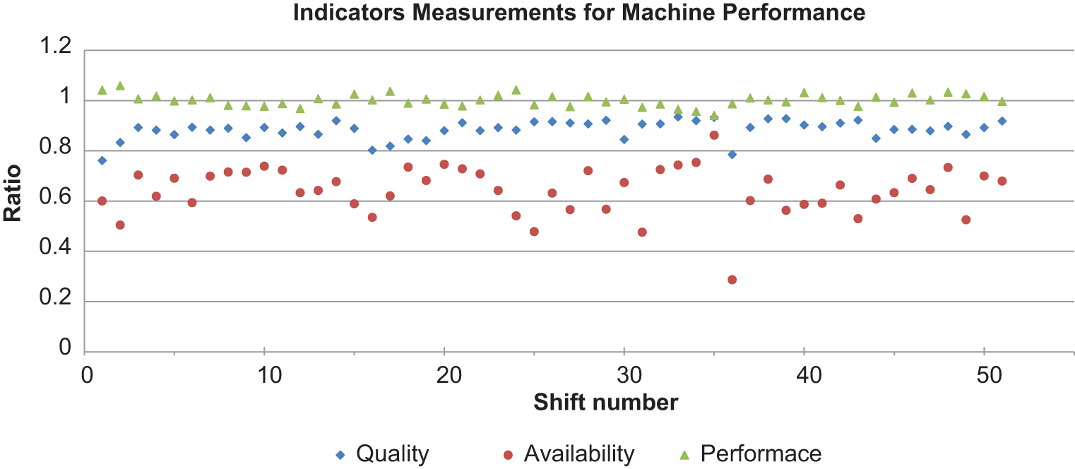
Scatterplot of Availability (R1), Productivity (R2) and Quality (R3).

Figure 10.

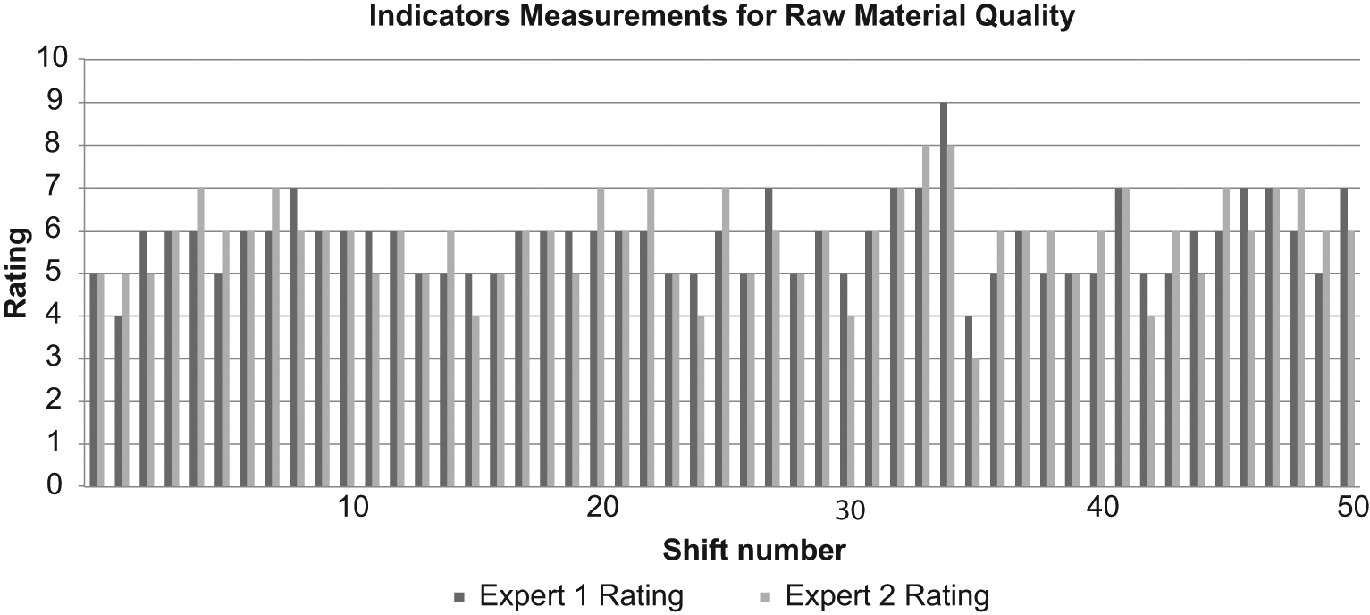
Scatterplot of Expert 1 Rating (F1) and Expert 2 Rating (F2).

Using the PLS-PM algorithm for PLS Regression of Mode B analysis as outlined by Esposito Vinzi et al. ¹⁴ (PLS Handbook, p. 56), the first step is to assign an arbitrary weight $w_{\mathrm{pq}}$ to each of the $p\mathrm{th}$ indicator belonging to the corresponding $q\mathrm{th}$ component. Next, the outer estimate ${\nu }_q$ of the $q\mathrm{th}$ component is obtained as a linear combination of its corresponding indicators

$${\nu }_q\propto \pm \sum _{p=1}^{P_q}{\omega }_{\mathrm{pq}}{x}_{\mathrm{pq}}$$

where $x_{\mathrm{pq}}$ is the observation for the $p\mathrm{th}$ indicator belonging to the corresponding $q\mathrm{th}$ component. In this case

$$\begin{array}{cc}\multicolumn{1}{c}{}& {\nu }_{\mathrm{Machine}\mathrm{Performance}}\propto \pm {\omega }_{R1}{x}_{R1}\pm {\omega }_{R2}{x}_{R2}\pm {\omega }_{R3}{x}_{R3}\hfill \\ \multicolumn{1}{c}{}& {\nu }_{\mathrm{Raw}\mathrm{Material}\mathrm{Quality}}\propto \pm {\omega }_{F1}{x}_{F1}\pm {\omega }_{F2}{x}_{F2}\hfill \end{array}$$

The choice of ‘±’ sign is selected such that the indicators are coherent with the meaning of the component. The next step is to obtain the standardised inner estimate ${\vartheta }_q$ of the $q\mathrm{th}$ component by analysing its adjacent latent variables $Q\prime$

$${\vartheta }_q\propto \sum _{q\prime =1}^{Q\prime }{e}_{\mathrm{qq}\prime }{\nu }_{q\prime }$$

Under the structural scheme, the inner weight $e_{\mathrm{qq}\prime }$ is equal to the regression coefficient between the outer estimate ${\nu }_q$ and the adjacent outer estimate ${\nu }_{q\prime }$ . Two alternative schemes – factorial scheme or centroid scheme – can be selected at this stage. However, with only two latent variables in the model, all schemes will yield identical result, and thus, no further discussion will be made on this topic. The algorithm then goes on to update $w_{\mathrm{pq}}$ . In Mode B analysis, the vector $w_q$ of the weights $w_{\mathrm{pq}}$ is updated using

$$w_q={\left(\frac{X{\prime }_q{X}_q}{N}\right)}^{-1}\frac{X{\prime }_q{\vartheta }_q}{N}$$

where $X_q$ is the observation matrix of the $q\mathrm{th}$ component and the observations are scaled by the sample size $N$ . As for this case

$$\left(\begin{array}{c}\hfill w_{R1}\hfill \\ \multicolumn{1}{c}{w_{R2}}\\ \multicolumn{1}{c}{w_{R3}}\end{array}\right)={\left(\frac{X{\prime }_{\mathrm{MP}}{X}_{\mathrm{MP}}}{51}\right)}^{-1}\frac{X{\prime }_{\mathrm{MP}}{\vartheta }_{\mathrm{MP}}}{51}$$

$$\left(\begin{array}{c}\hfill w_{F1}\hfill \\ \multicolumn{1}{c}{w_{F2}}\end{array}\right)={\left(\frac{X{\prime }_{\mathrm{RMQ}}{X}_{\mathrm{RMQ}}}{51}\right)}^{-1}\frac{X{\prime }_{\mathrm{RMQ}}{\vartheta }_{\mathrm{RMQ}}}{51}$$

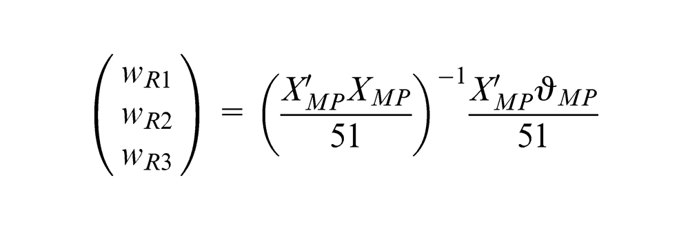
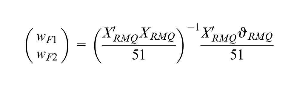
The algorithm then continues to alternatively obtain outer and inner estimates until the iteration converge. Upon convergence, the standardised component scores ${\hat{\xi }}_q$ for the $q\mathrm{th}$ component are calculated as the linear combination of its corresponding indicators

$${\hat{\xi }}_q=\sum _{p=1}^{P_q}{\omega }_{\mathrm{pq}}{x}_{\mathrm{pq}}$$

Finally, simple regression is used to determine the path coefficient between the two standardised component scores. Figure 11 shows the converged model for Mode B for this study.

Figure 11.

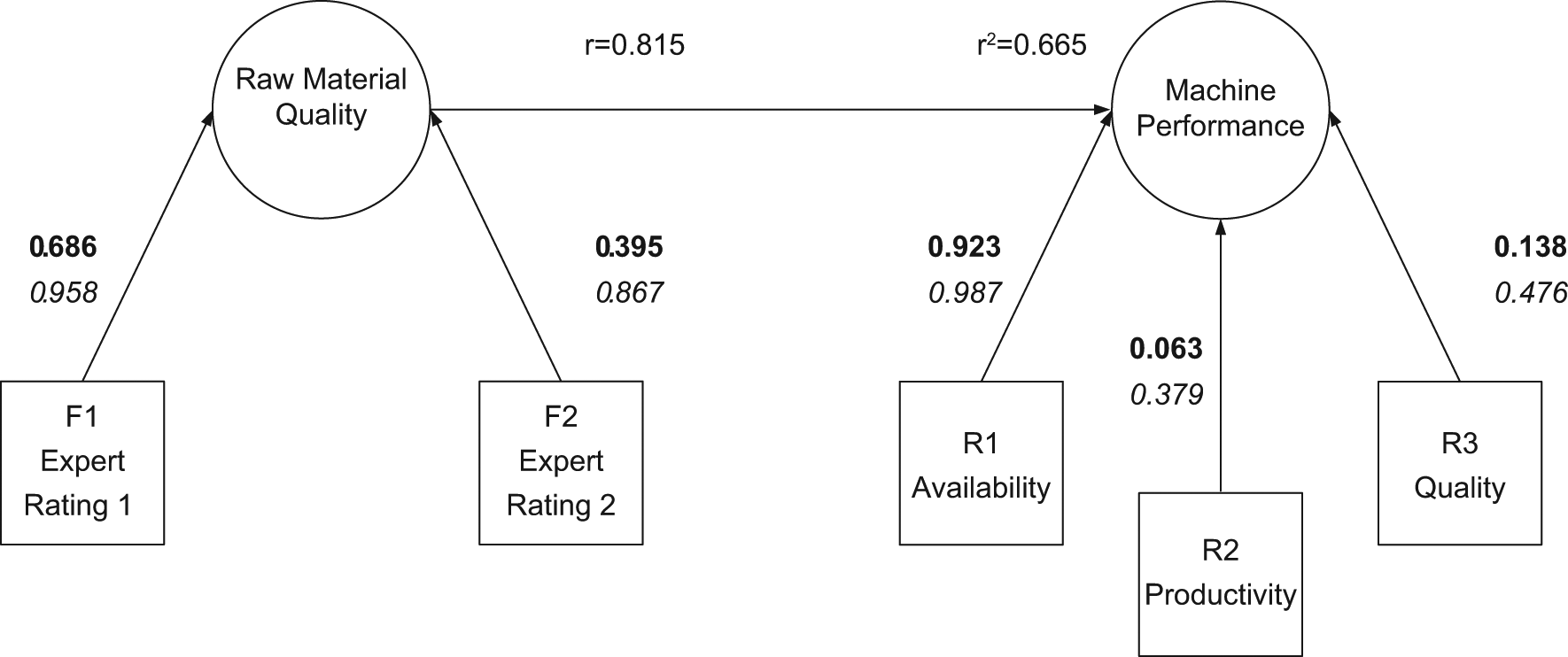
Mode B analysis of raw material quality and machine performance.

The results suggest that there was a moderate regression coefficient between the raw material quality and machine performance with R² of 0.665. The data were also resampled 500 times using Bootstrap^15,16 to establish the 95% confidence intervals for R² as (0.479, 0.834). This suggests that the raw material quality is a significant predictor for machine performance. In addition, the higher weight value of Expert 1 suggests that their judgement on this raw material would provide better prediction for machine performance. Expert 1 would be the preferred expert for assessing this raw material quality. The moderate coefficient between also suggests that further studies on this area are necessary. In order to uncover the variability of quality of this raw material, different components may be constructed using operating variables and parameters from the manufacturing phase of this raw material. Once these critical factors of raw material are found, it is then possible to construct a structural equation that predicts the relationship between critical operating variables with machine performance which will be discussed in future papers.

Statistical analysis no longer lives in a vacuum. The availability of large data sets and easily accessible software allows any armchair expert to find a statistically significant result that is completely insignificant. For many businesses proving a change to be statistically significant at the 95% level has no tangible meaning. Business is driven by the underlying motive to make a profit, any changes that assist with this are of interest, irrespective of their statistical significance. In the previous example, a particular raw material quality accounted for approximately 66.5% of the variance in the machine performance. As a single measure this could be a very important outcome, if the cost to improve the raw material is relatively low, and a small improvement in the machine performance produces a large profit. Equally, the fact that the quality of the raw materials accounts for 66.5% of the variance of OEE may be of little benefit if there is only one supplier in the market.

Engineering is uniquely placed to stand at the crossroads of business and statistical analysis. Engineers should be able to interpret the outcomes of the analysis and tie these with the needs of business. Moving away from statistical significance as the benchmark of success requires new, innovative approaches to reporting and decision making. Often this comes through hard fought experiences. In our next study, we will outline a framework for assessing the results outside of the traditional boundary of statistical significance.