Tool path design for enhancement of accuracy in single-point incremental forming

Abstract

One of the variants and simplest form of incremental sheet metal forming process is single-point incremental forming in which a spherical ended tool is used to form features on one side of the initial plane of the sheet. Dimensional deviation is observed in the region of component opening (due to sheet bending) and at the wall as well as base regions. This article presents a methodology to minimize the dimensional deviation in the wall and base regions of single-point incremental forming formed components. The authors observed that the sheet deflection due to axial force and tool deflection due to radial force are the two main factors leading to the geometric deviation in wall as well as base regions. An analytical model has been developed for estimating these two deflections. These deflection values are incorporated in the tool path generation, and the components formed using the compensated tool path resulted in acceptable dimensional accuracy in the wall region. Force predictions carried out by force equilibrium method are used to calculate the deflection compensations as its predictions are in reasonably good agreement with the force predictions of finite element analysis and experimental measurements. Significant improvement in accuracy is achieved by using the deflection compensated tool paths.

Introduction

Incremental forming (IF) is an innovative technology in the field of sheet metal forming, which satisfies the requirement of customized production with cost reduction. The basic feature of IF is the localized deformation of the sheet using simple spherical ended tool, which moves along the predefined path generated from the computer-aided design (CAD) geometry of the component. It avoids the need for component-specific tooling, and a wide variety of three-dimensional (3D) shapes can be produced using a three-axis computer numerical control (CNC) machine and the component-specific tool path. The advantages of IF are the increased formability, lower forming forces and low cost along with component-independent tooling. ¹ One of the variants of incremental sheet metal forming process is single-point incremental forming (SPIF) in which a spherical ended tool is used to form features on one side of the initial plane of the sheet.

Many authors have studied the SPIF process and tried to improve the dimensional accuracy by incorporating various strategies. Ambrogio et al. ² have studied the effect of tool diameter and incremental depth on the dimensional accuracy in SPIF by conducting series of experiments and concluded that the accuracy is better while using smaller diameter tools and lower incremental depths. Use of lower incremental depth increases the forming time. In addition, it was also stated that bending in the absence of a backing plate/die is a major cause for geometrical inaccuracies. They proposed a modified tool path to enhance the accuracy by forming a component with a smaller opening and higher wall angle than the desired up to some depth and then forming the remaining component with the desired angle. Conical components formed using the above strategy enhanced the accuracy by reducing the bending near component opening. Ambrogio et al. ³ also reported the deviation in the base region and termed it as ‘pillow effect’. They have carried out statistical analysis of truncated pyramid-shaped component to obtain errors as a function of process variables. They compensated for the same by over-bending. This in turn increases the bending at the opening region although it reduces the deviation in the wall region. Verbert et al. ⁴ reported maximum profile deviation of 1 mm in pyramidal components using modified tool path strategy based on feature detection method. Instead of modifying the tool path directly after gathering information about how different feature behaves under processing conditions, the CAD model itself is modified and tool path is generated based on modified model. They used STereoLithography (STL) format for input, and it is well known that it has inherent inaccuracies due to chordal errors. Duflou et al.^5,6 made use of laser-assisted local heating, slightly ahead of the tool to form cone-shaped components of 65Cr2 sheets. Due to the local heating, reduction in forming forces, spring back and plastic deformation outside the tool contact zone is observed. This leads to an overall reduction in profile deviation from 3.6 to 1.5 mm. Allwood et al. ⁷ demonstrated closed-loop control in SPIF process that uses spatial impulse responses to control the accuracy. They predicted impulses by fitting a cumulative Weibull distribution to experimental impulses for a cone geometry and then formed similar cones with ±0.2 mm error. Experimentally predicting the spatial impulse responses would be a costly affair as it requires very large number of experiments and finite element analysis (FEA) would be a slow and time-consuming exercise. Their methodology has to be repeated for all geometries and materials to use in practice. Bambach et al. ⁸ applied multistage forming (four-stage forming) for reducing the local spring back and reported maximum error of 0.41 mm in place of 2.5 mm in single-stage forming. This reduction is mainly due to reduction in instantaneous forces. Note that the components considered can also be produced using single-stage forming without failure, hence the forming time increases significantly. Verbert et al. ⁹ made an attempt to compare dimensions of components formed using robots and CNC machines. Because robots are less stiffer than CNC machines, components formed by robots have more dimensional inaccuracy. To enhance dimensional accuracy of components formed using robot, they applied compensations to the end-effector movement based on measured forces and joint compliance and then formed a 50°cone using robot and observed an improvement in deviation from 1.2 to 0.7 mm (close to that achieved on a CNC machine − 0.6 mm). In addition, there are many attempts to enhance the accuracy in the component opening region due to bending by using a back-up plate having size and shape close to the component opening. Significant reduction in error due to bending at component opening is reported^2,5,6,10 with the use of backing plate/pattern support.

Literature presented above indicates that the main drawback of the SPIF process is the poor accuracy. ¹ The deviations observed in the process are not only due to the inevitable bending near the opening region but also due to the deviation in the wall region as well as component height. This work is an attempt to develop a simple mathematical model based on classical mechanics to improve the dimensional accuracy in SPIF process by compensating the tool and sheet deflections in addition to tool radius compensation while generating tool path.

Compensation methodology

The first step in implementing the compensation methodology is to predict the forming forces with reasonable accuracy in axial, tangential and radial directions. In this work, a simple force equilibrium–based method along with thickness prediction method developed by Bhattacharya et al. ¹¹ is used to predict forces. This method can predict forces with reasonably good accuracy to those predicted by FEA. Tool deflection due to radial force and sheet deflection due to axial force are vectorially added, and corresponding compensation is applied to the tool path obtained from CAD model. The methodology is elaborated in the following paragraphs.

Force prediction

Non-uniform thickness distributions of the formed geometries are obtained by following the methodology developed by Bhattacharya et al. ¹¹ This methodology considers the overlap (some part of the material in SPIF gets deformed repeatedly due to overlap) in deformation zone while calculating the thickness. The amount of overlap depends on the wall angle, incremental depth and tool radius. Considering the overlap, increased length of each small region is obtained. Imposing volume constancy, thicknesses of all elements are obtained. Considering plane strain deformation and von Mises yield criterion, strain components are calculated and then the equivalent stress at that section is obtained using the stress–strain relation of material being deformed. Using the equivalent stress calculated above, stress components in thickness, meridional and circumferential directions are calculated using equations (1)–(3), respectively^11,12

$${\sigma }_t=-\frac{2{\sigma }_{\mathrm{eq}}}{\sqrt{3}}\left(\frac{t}{R_t+t}\right)$$

(1)

$${\sigma }_{\varphi }=\frac{2{\sigma }_{\mathrm{eq}}}{\sqrt{3}}\left(\frac{R_t}{R_t+t}\right)$$

(2)

$${\sigma }_{\theta }=\frac{{\sigma }_{\mathrm{eq}}}{\sqrt{3}}\left(\frac{R_t-t}{R_t+t}\right)$$

(3)

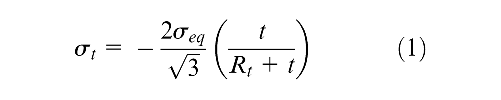
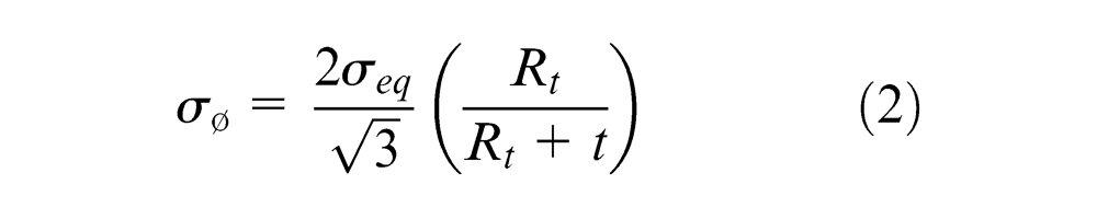
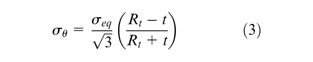
where σ_eq is the equivalent stress, R_t is the tool radius and t is the sheet thickness at any instant.

The force components (thickness F_t, meridional $F_{\varphi }$ and circumferential F_θ) are estimated by estimating contact area between tool and sheet at any instant. Contact area has been approximated as a rectangle (as shown in Figure 1(a) with length l and width w) based on contact pressure distribution ¹³ observed during FEA. Area of the contact is assumed as half the area of contact during indentation. Length of this rectangle is equal to the contact length ( $\widehat{\mathrm{ABC}}$ in Figure 1(b)) in meridional direction. $l=R_t(\alpha +\beta )$ where α is the wall angle and $\beta ={\cos }^{-1}(1-\Delta z/R_t)$ is the groove angle (see Figure 1(b)) due to indentation. Stress components ( ${\sigma }_t,{\sigma }_{\varphi },{\sigma }_{\theta }$ ) obtained above are assumed to be acting uniformly over the contact area to determine the corresponding force components $(F_t,F_{\varphi },F_{\theta })$ . Force components ( $F_t,F_{\varphi },F_{\theta }$ ) are then resolved to find the components along axial ( $F_z$ ), radial ( $F_r$ ) and tangential $(F_{\mathrm{tg}})$ directions (see Figure 1(a)).

Figure 1.

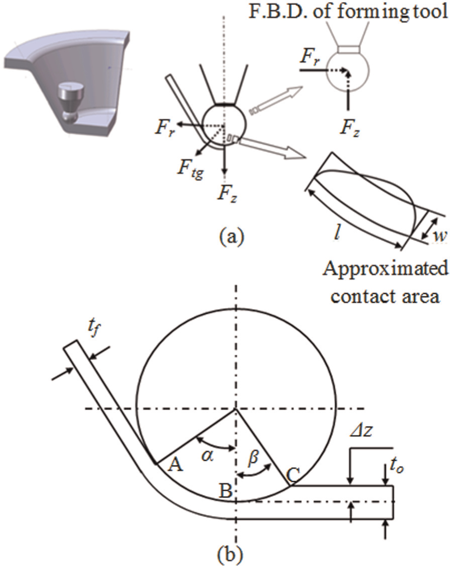
(a) Schematic representation of forces acting during single-point incremental forming and approximated contact geometry and (b) groove angle in indentation.

Tool deflection

Due to the radial and tangential forces acting on forming tool, tool gets deflected and results in forming smaller cross-sectional profile than the intended one. Considering the radial force acting on the tool, the amount of tool deflection ( ${\delta }_{\mathrm{tool}}$ ) is calculated using equation (4) and assuming the tool to be a cantilever

$${\delta }_{\mathrm{tool}}=\frac{F_r{l}^3}{3\mathrm{EI}}$$

(4)

where F_r is the radial force (shown in Figure 1), l is the length of overhang (distance from spindle collet to tool tip), E is Young’s modulus of tool material (taken as 200 GPa for EN32) and I is the moment of inertia. Although the tool geometry deviates from cylindrical geometry (near the portion where spherical ball is mounted), it is assumed as a regular cylinder to calculate moment of inertia ( $I=\pi d_s^4/64$ ) where d_s is the shank diameter of the tool. Only radial force is considered to calculate the deflection as the radial deflection (0.0001 mm) due to tangential force is very small compared to radial deflection (0.4416 mm) due to radial force (parameters used to calculate deflections are 60° cone with 12.7 mm tool and Δz = 0.5 mm).

Sheet deflection

The elastic deflection of sheet at any instant of SPIF (due to the force acting along tool axis at the tool–work contact location) is estimated by considering sheet to be peripherally clamped and deformation is imposed by the tool moving in spiral path (out-to-in). Loading condition in incremental sheet forming is analogous to a concentrically loaded circular plate with clamped edges as shown in Figure 2.

Figure 2.

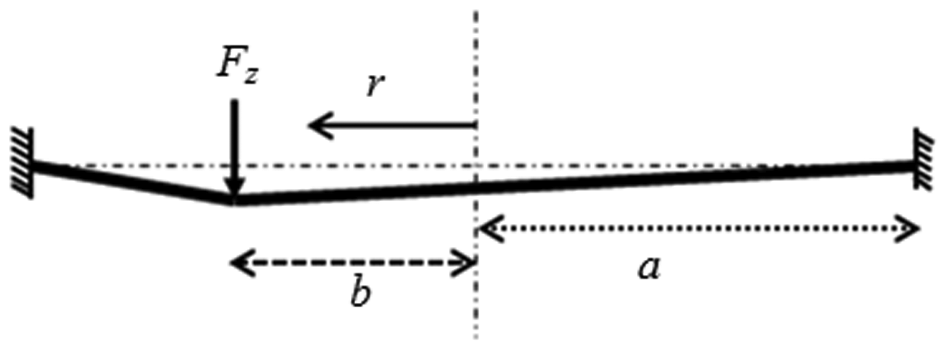
Schematic representation of loading condition and parameters used for sheet deflection calculation.

Figure 3(a) schematically represents the profile of the component at any instant under point load (Fz) at P. When the tool (moving in spiral or contour path) reaches diametrically opposite point P ¹ , point P undergoes elastic recovery (Figure 3(b)). To form the accurate geometry, one has to compensate for the recovery that occurs at each location during deformation.

Figure 3.

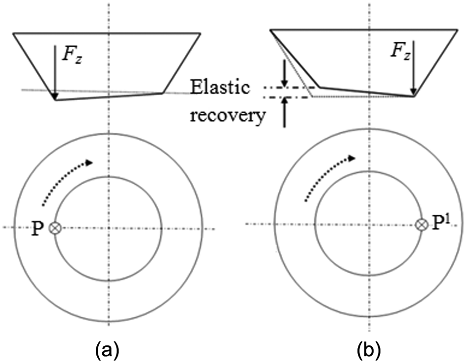
Illustration of sheet behaviour during one contour movement. (a) component profile when tool is at point P and (b) elastic recovery of sheet when tool moves to diametrically opposite point P1.

The estimation of elastic recovery can be carried out utilizing the theory of sheet deflection. Middle surface of the sheet (at half of sheet thickness) is assumed to be neutral surface, and the deflections are assumed to be small as compared to the sheet thickness. Under the above assumptions, deflection of the sheet in the inner region (r≤b) is given by equation (5) ¹⁴

$$\begin{array}{c}\multicolumn{1}{c}{{\delta }_{\mathrm{sheet}}=\frac{F_z}{8\pi D}[-(r^2+b^2)\ln \left(\frac{a}{b}\right)+(r^2-b^2)+\frac{1}{2}(1+\frac{b^2}{a^2})(a^2-r^2)]}\end{array}$$

(5)

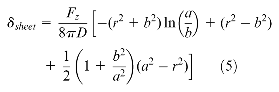
where F_z is the axial force acting along the tool axis (refer Figure 1), a is the distance from the centre of the component to the clamped edge, b is the component opening radius (at point of loading) and D is the flexural rigidity of sheet material calculated as

$$D=\frac{E_s{t}^3}{12(1-{\nu }^2)}$$

where E_s is Young’s modulus of sheet material (= 70 GPa for Al5052 alloy), t is the sheet thickness and ν is Poisson’s ratio.

Due to the symmetry of sheet and its boundary conditions, the deflection produced in the inner region (r≤b) by the force F_z depends only on the magnitude of F_z and the radial distance (r) where it acts. The deflection remains unchanged if the load moves to other location provided the radial distance remains the same. ¹⁴

Compensated tool path generation

Required tool path is generated from CAD model by adopting the methodology developed by Malhotra et al. ¹⁵ In this methodology, CAD model is sliced to get contour contact path, spiral contact path is generated from contour path and then tool radius compensation is applied to get spiral tool path. Note that their ¹⁵ methodology takes care of tool radius compensation only. The deflection (δ) is taken as the vectorial sum of tool deflection (δ_tool) and sheet deflection (δ_sheet). Appropriate compensation is applied to spiral tool path to generate compensated tool path. Figure 4 shows the comparison between the ideal profile and the compensated tool path. Applying the compensations iteratively has been tried and found the improvement to be negligible. Further details regarding the same are provided in section ‘Validation’.

Figure 4.

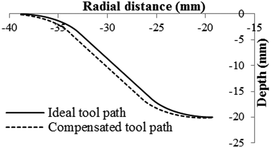
Comparison of ideal tool path and compensated tool path.

Validation and experimental procedure

The force prediction methodology and tool path compensation methodology presented in the above section are implemented using MATLAB. To validate the proposed methodology, axial force component predicted by proposed methodology is compared with FEA prediction and experimentally measured value, whereas radial and tangential components of the force and sheet spring back predictions are compared with FEA predictions.

Nomenclature

Profile of a component is divided into four regions (Figure 5) for better understanding. They are as follows: (1) top fillet, (2) wall region, (3) bottom fillet and (4) base region. Component opening region is also shown in Figure 5.

Figure 5.

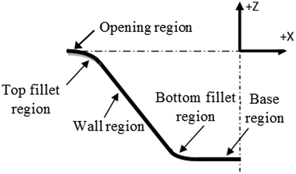
Component zones and their nomenclature.

FEA

FEA of SPIF of 60° wall angle truncated cone with 12.7 mm tool diameter and 0.5 mm incremental depth is carried out using ABAQUS. The deformation analysis is carried out using shell elements. Tool is considered as analytically rigid and sheet as deformable.

Comparison between finite element–predicted profile and ideal profile is shown in Figure 6. The deviation due to bending of sheet in the opening region that can be observed in Figure 6 is an inherent limitation of SPIF. It can be observed that the deviation due to bending is negligible after reaching certain depth, that is, wall and base regions. It can also be observed that the cross-sectional profile of formed component is smaller than the ideal cross-sectional profile in wall and base regions.

Figure 6.

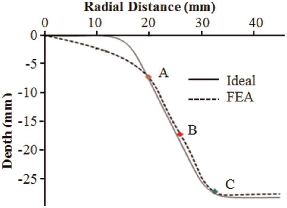
Comparison of FEA-predicted profile with ideal profile.

FEA results are further analysed to understand the deformation history of sheet during SPIF and the deviation of profile in wall region. Displacement history of three nodes at different locations A, B and C shown in Figure 6 is studied. Figure 7 shows the progressive vertical displacement of the above nodes during deformation process. Each cyclic portion of any curve in Figure 7 corresponds to a tool movement of one segment of spiral shown in Figure 7 (50 cyclic portions corresponds to 50 such spiral segments of tool path shown in Figure 7).

Figure 7.

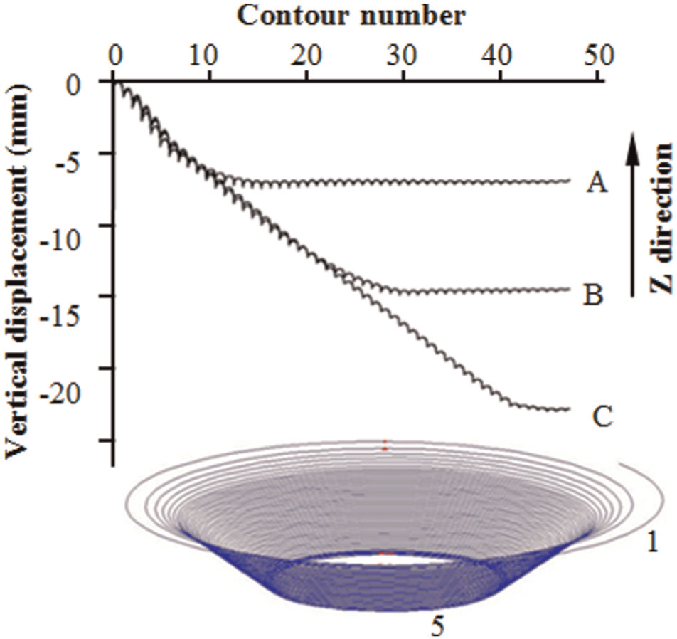
Displacement history of nodes (A, B and C of Figure 6) at different tool locations (truncated cone of 60° wall angle, opening diameter 33 + 6.35R fillet, height 25 mm and incremental depth 0.5 mm).

Figure 8(a) shows the change in profile of the component during the tool movement along one spiral segment. The tool comes in contact with node (A) (Figure 8(b)) corresponding to tool location T1 (Figure 8(c)) on the tool path. When the tool moves to the diametrically opposite location T2, node A moves up (to new location A1) due to local spring back and bending recovery (elastic) (Figure 8(b)). When the tool moves to T3, it again comes in contact with the node (A) due to overlap of contact zone and it moves to a new location A2. Distance between A and A2 along z-direction is equal to the incremental depth. The tool completes one segment along the spiral tool path while node A moves to A2. The distance between A and A1 in z-direction gives the deviation in profile due to local spring back and bending recovery. Figure 8(d) shows the complete history of recovery taking place during movement of tool over a single spiral segment, and it indicates that as soon as the tool moves away from location A, it starts moving upwards and the rate of recovery decreases till the tool reaches the diametrically opposite position T2. Then, it starts moving downwards and reaches location A2 corresponding to the next position of tool (T3). This process continues throughout the forming process, but the amount of recovery decreases after the initial forming stage and the same can be observed in Figure 7. The maximum spring back value observed due to elastic bending recovery and local spring back is equivalent to 0.46 mm (for 60° cone, tool diameter 12.7 mm and step size 0.5 mm).

Figure 8.

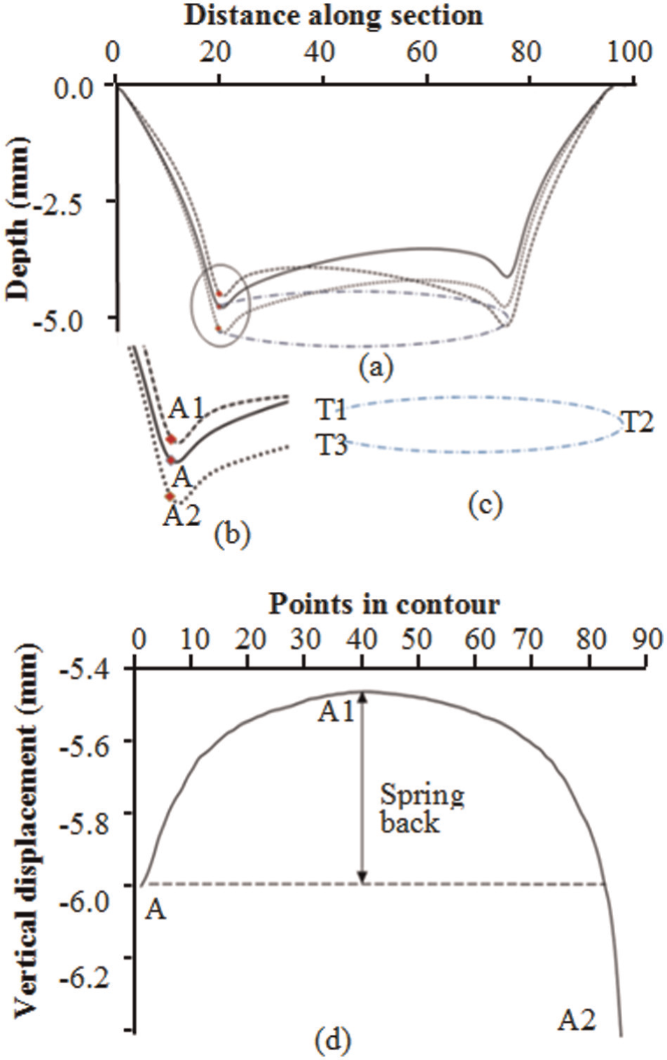
Spring back and profile deviation during tool movement of one segment of spiral (truncated cone of 60° wall angle, opening diameter 33 + 6.35R fillet, 25 mm height and incremental depth 0.5 mm). (a) component profiles with tool positions T1, T2, T3, (b) contact point locations with tool positions T1, T2, T3, (c) tool positions T1, T2, T3 on a segment of spiral and (d) path traced by contact point while tool moved one segment of spiral.

A plot of forces predicted by FEA is shown in Figure 9. Average axial force around 1100 N, average radial force around 450 N and average tangential force around 70 N are predicted by FEA.

Figure 9.

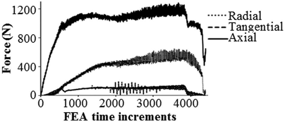
Force prediction through FEA (for 60° cone, 12.7 mm tool diameter and 0.5 mm incremental depth).

Experimental procedure

Components are formed on a custom-built double-sided incremental forming (DSIF) machine (Figure 10) capable of forming complicated 3D components using tools on both sides of the initial plane of the sheet. The machine has two tools one on either side of sheet, but only top tool is used to perform SPIF. A single-component button-type load cell is mounted on the forming tool to measure the axial component of the forming force.

Figure 10.

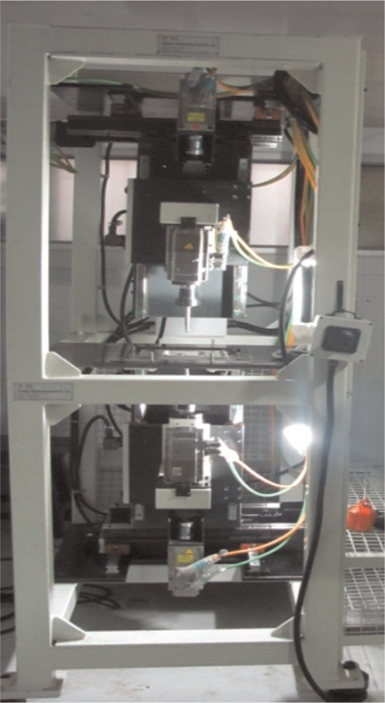
Incremental forming machine used in this work (designed and developed at Indian Institute of Technology Kanpur).

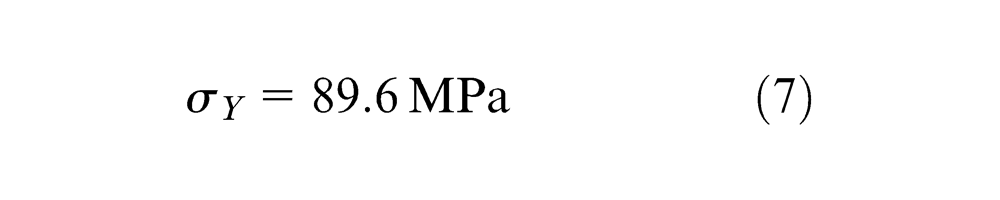
Aluminium 5052 sheet of 0.88 mm thickness is used to carry out all the experiments. Its stress–strain relation is obtained using tensile test as

$${\sigma }_{\mathrm{eq}}=332{\epsilon }_{\mathrm{eq}}^{0.12}$$

(6)

$${\sigma }_Y=89.6\text{MPa}$$

(7)

Preliminary experiments are carried out by forming truncated conical shapes of 60° wall angle with 12.7 mm tool diameter and 0.5 mm incremental depth without applying deflection compensation. The axial force (F_z) measured experimentally is 1080 N.

Validation

Axial, radial and tangential forces predicted by force equilibrium method explained in section ‘Compensation methodology’ for 60° cone, 12.7 mm tool diameter and 0.5 mm incremental depth (same as FEA and experiment) are F_z (max) = 1040 N, F_r (max) = 400 N and F_tg (max) = 82 N, and the sheet deflection obtained is 0.47 mm. Comparison of predictions with FEA predictions and experimental measurement is given in Table 1.

Table 1.

Comparison of predicted forces.

	Force equilibrium prediction	FEM prediction	Experimental measurement
Fz (N)	1040	1100	1080
Fr (N)	400	450
Ftg (N)	82	70
Spring back	0.47 mm	0.46 mm

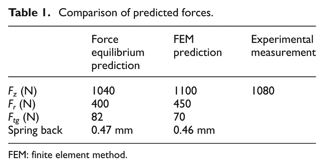
FEM: finite element method.

Comparisons presented in Table 1 indicate that the force and spring back predictions by force equilibrium methodology are in good agreement with FEA predictions. Axial force predicted by force equilibrium methodology is in good agreement with experimentally measured value. Hence, the proposed methodology is used in this work to calculate compensations to generate compensated tool paths. Prediction of compensation for deflection is an iterative process, but the following discussion indicates that it will not result in any considerable improvement. The deflections in the wall region obtained by considering the predicted forces for 60° wall angle cone with 12.7 mm tool diameter and 0.5 mm incremental depth are δ_tool = 0.4416 mm due to radial force and δ_sheet = 0.4385 mm due to axial force giving total deflection of δ = 0.6223 mm. The deflections obtained by considering the increase in wall angle due to compensation and corresponding increase in predicted forces are δ_tool = 0.4466 mm and δ_sheet = 0.4386 mm giving total deflection of δ = 0.6259 mm. It can be seen that there is a negligible increase in deflections (Δδ_tool = 0.005 mm, Δδ_sheet = 0.0001 mm and Δδ = 0.0036 mm) in second iteration itself, so the compensations are estimated without using iterative process.

Components formed

Truncated conical shapes with wall angles 30°, 40°, 50° and 60° are formed while testing the methodology in which results of only 60° and 30° cones are presented in this article. Two more components are formed to validate the methodology for different angles. First one is a funnel shape with wall angle varying and the second is a free form with elliptical opening.

The funnel shape used is an axisymmetric revolution geometry (cross section shown in Figure 11(a)) with wall angle varying from 25° (at tip) to 60° as the depth increases, opening radius of 37 mm, bottom fillet radius of 6.35 mm (equivalent to tool radius) and depth of 25 mm. The free-form shape (two views are shown in Figure 11(b)) has elliptical opening with major axis 80 mm, minor axis 70 mm and depth 26 mm. Note that the free-form shape chosen does not have flat base.

Figure 11.

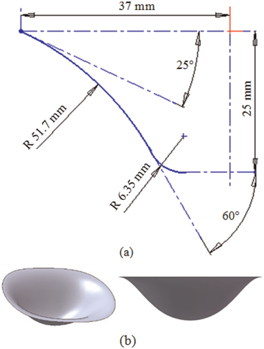
(a) Funnel-shaped cross-sectional profile and (b) CAD model of free-form shape.

Results and discussion

Validation of force and deflection predictions presented in section ‘Validation and experimental procedure’ indicates that the methodology proposed during this work can be used to calculate the deflections to generate compensated tool paths to improve the accuracy of components during SPIF. Various geometries are formed with and without applying the compensations. The description of geometries formed is given in section ‘Components formed’. Tool diameter of 12.7 mm and incremental depth of 0.5 mm are used in all the experiments. Profiles are measured by keeping the component in clamped position. Semi-automatic three-axis coordinate measuring machine (CMM) (Accurate CMM Spectra 5.6.4, accuracy 0.1 µm) is used for profile measurement.

60° conical component

First, a truncated cone of 60° wall angle is formed without considering any compensation for deflections. Note that 60° wall angle is close to the forming limit for Al5052 as reported earlier. ¹¹ Figure 12 shows the comparison between ideal and formed profiles. It can be observed that the measured profile deviates from the ideal profile in all regions. A significant amount of bending is observed near the top fillet/opening region. Maximum error of 1.2 mm is observed in the wall region.

Figure 12.

Comparison of measured and ideal profiles (with and without compensation) (truncated cone of 60° wall angle, opening diameter 33 + 6.35R fillet, 25 mm height, Al5052 0.88 mm thick, tool diameter 12.7 mm and incremental depth 0.5 mm).

The same component is formed with deflection compensated tool path. It can be clearly seen from Figure 12 that there is a significant improvement in profile accuracy by using compensated tool path. Component formed using SPIF with deflection compensated tool path is in better agreement with the ideal geometry in the wall, bottom fillet and base regions. However, bending near top fillet/opening region is still present and is unavoidable in SPIF. Maximum error is reduced by 0.9 mm (1.2–0.3 mm) using the compensated path.

30°conical component

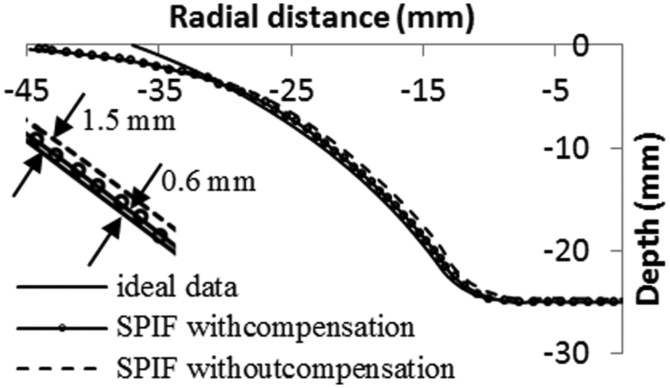
Similar to 60° component presented above, compensation methodology is applied to a cone with lower wall angle (30°) to study the accuracy. Ideal profile and measured profiles of components formed using tool paths without compensation (tool radius compensation applied) and with compensation (deflection compensation) are shown in Figure 13. Measured profile of component formed without compensation deviates in all the regions from the ideal profile, whereas component formed with compensation better matches with the ideal profile in all the regions except top fillet/opening region, where bending is still present. However, in the base region, maximum error of 0.3 mm is observed owing to pillow effect. This is due to the fact that during out-to-in movement, the tool pushes un-deformed material towards the centre whose effect is prominent when base region area is considerably small (close to the tool diameter). A remedy to this problem is to move the tools up to the centre of the component.

Figure 13.

Comparison of measured and ideal profiles (with and without compensation) (truncated cone of 30° wall angle, opening diameter 33 + 6.35R fillet, 25 mm height, Al5052 0.88 mm thick, tool diameter 12.7 mm and incremental depth 0.5 mm).

Funnel component

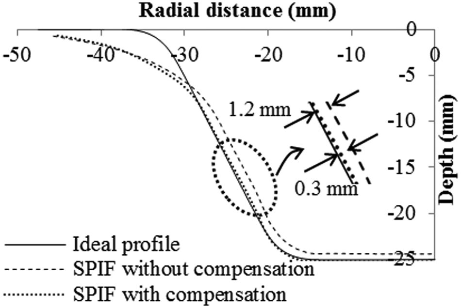
To further validate the compensation methodology, a funnel-shaped component with continuously varying wall angle is formed. Comparison between ideal and measured profiles is shown in Figure 14. For the funnel component, the deflections are calculated as per the local wall angle. This gives a varying compensation at different locations as per the component profile. It can be seen from Figure 14 that in the funnel formed using SPIF without compensation, the profile deviates from the ideal in all the regions and maximum error of approximately 1.5 mm is observed. Although profile accuracy is enhanced with compensation methodology, maximum error of about 0.6 mm is observed. Bending near top fillet region remains unavoidable.

Figure 14.

Comparison of measured and ideal profiles for funnel component with varying wall angle (wall angle varying from 25° to 60°, opening diameter 33 + 6.35R fillets, 25 mm height, Al5052 0.88 mm thick sheet, tool diameter 12.7 mm and incremental depth 0.5 mm).

Free-form component

The tool path methodology reported here is tested for a wide variety of geometries including free-form surfaces. Figure 15 shows the picture of free-form shape component whose geometry is given in section ‘Components formed’ and shown in Figure 11(b).

Figure 15.

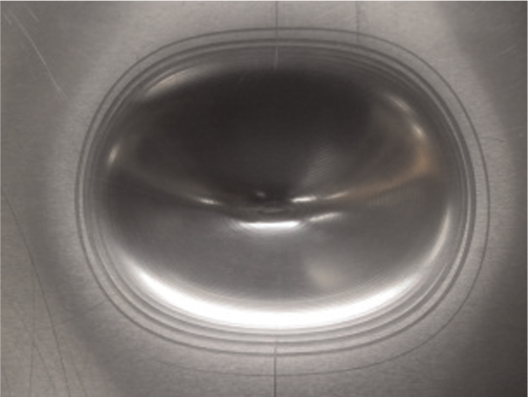
Picture of free-form component formed.

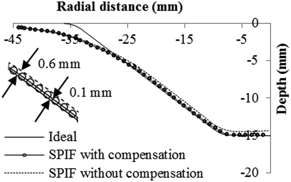
Comparison of ideal profile along the major axis of the component with that of component formed without applying tool path compensations and with applying tool path compensations is shown in Figure 16. It can be clearly seen from Figure 16 that actual profile of component formed by applying compensation is very close to the ideal profile. Maximum error of 0.37 mm has been measured at the bottom-most portion of the component. The component formed without compensation lies completely inside the ideal geometry except at component opening and has a maximum error of 1.5 mm.

Figure 16.

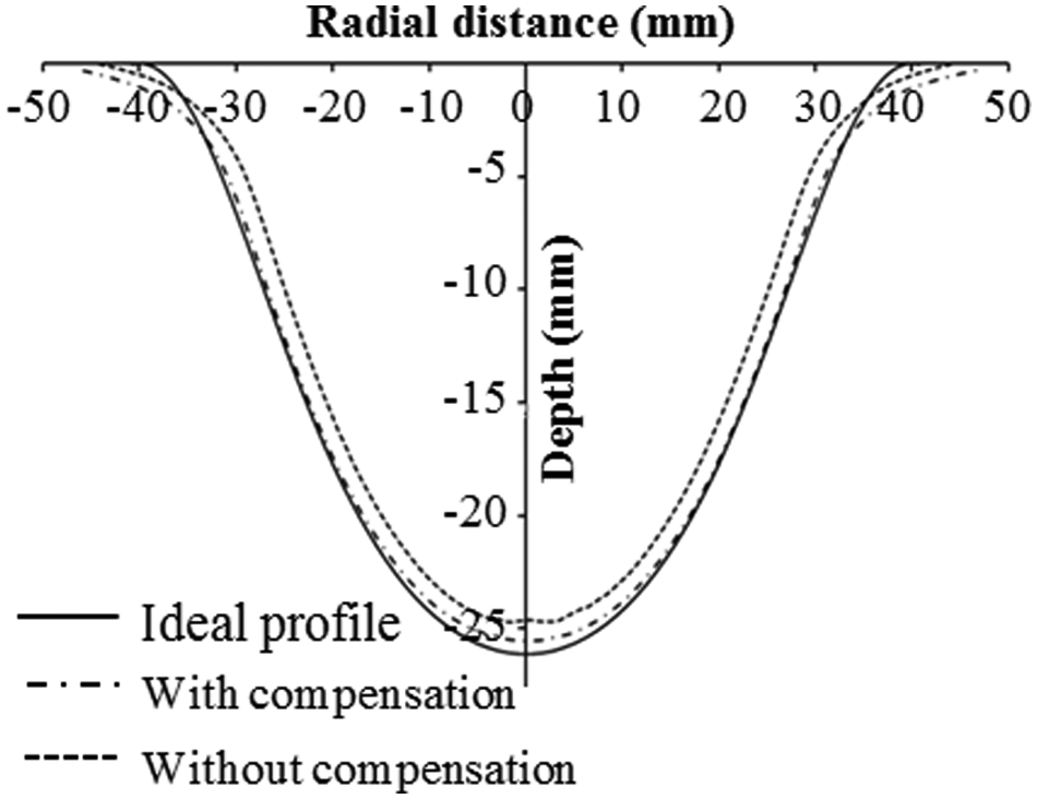
Comparison of measured and ideal profiles of free-form component (elliptical opening with major axis 80 mm, minor axis 70 mm, depth 26 mm, Al5052 0.88 mm thick, tool diameter 12.7 mm and incremental depth 0.5 mm).

Further work to reduce the bending in top fillet region is in progress by using DSIF. In this variant of incremental sheet forming, a second tool that is independently controlled is used on the other side of the sheet.

Conclusion

The results presented in this article indicate that the improvement in accuracy by applying deflection compensation is significant in component wall and base regions. Reduction in error of 0.9 mm (from 1.2 to 0.3 mm) is achieved in case of 60° wall angle component and reduction in error of 0.5 mm (from 0.6 to 0.1 mm) is achieved in case of 30° wall angle component. The methodology has improved accuracy significantly in case of components with varying wall angle and free-form geometry also.

Future work

Further work is in progress to enhance the accuracy levels using DSIF, that is, reducing bending near top fillet region.