Using modified grey forecasting models to forecast the growth trends of green materials

Abstract

The use of green materials reflects the notion that production materials should generate minimal environmental pollution through various efforts, including the design and development of low-pollution materials, innovation and improvement of low-pollution manufacturing processes, and recycling and reuse of materials. The development of green materials is an important part of corporate social responsibility. Companies need to use resources legitimately and have environmental protection responsibility. Forecasting the growth trends of green copper clad laminate material is crucial for manufacturers of printed circuit boards and green copper clad laminates. The main purpose of this study was to forecast the growth trends of green electronic materials. The industry sample investigated in this study only numbered 14. Because of the limited sample of historical data, the data distribution did not exhibit a normal distribution. Prediction methods for large data sets were not suitable for this study. Thus, three grey forecasting models (i.e. the grey model(1,1), non-linear grey Bernoulli model(1,1), and grey Verhulst model) were adopted for theoretical derivation and scientific verification. The results yielded by these methods were compared with the results of regression analysis to verify the forecasting accuracy and suitability of the three methods. The results indicated that for small data sets, the forecasting accuracy of the non-linear grey Bernoulli model(1,1) and grey Verhulst model was superior to that of the original grey model(1,1) as well as the regression analysis method.

Introduction

The use of green materials reflects the notion that production materials should produce minimal environmental pollution through various efforts, including the design and development of low-pollution materials, innovation and improvement of low-pollution manufacturing processes, and recycling and reuse of materials. To effectively reduce the impact that electrical and electronic products have on the environment and human life, the European Union (EU) enacted two directives in 2003: the Waste Electrical and Electronic Equipment (WEEE) Directive and the Restriction of Hazardous Substances in Electrical and Electronic Equipment (RoHS) Directive. The WEEE Directive requires manufacturers selling electrical and electronic products in the EU market to consider potential pollution problems caused by the disposal of waste products, to adopt environmentally friendly product designs that facilitate recycling, and to cover any expenses associated with waste recycling. The RoHS Directive restricts the use of six substances in the manufacturing of controlled electrical and electronic equipments: a maximum permitted concentration of 0.01% for lead (Pb), mercury (Hg), and cadmium (Cd), and a maximum concentration of 0.1% for hexavalent chromium (Cr^VI), polybrominated biphenyls (PBBs), and polybrominated diphenyl ethers (PBDEs). Additionally, in 2005, the EU issued the Eco-Design Directive for energy-using products. The Eco-Design Directive mandates that manufacturers incorporate eco-design requirements into product design and development according to the considerations of product life cycle to enhance product performance, reduce energy demands, and improve energy efficiency, thereby fulfilling high-level environmental requirements.

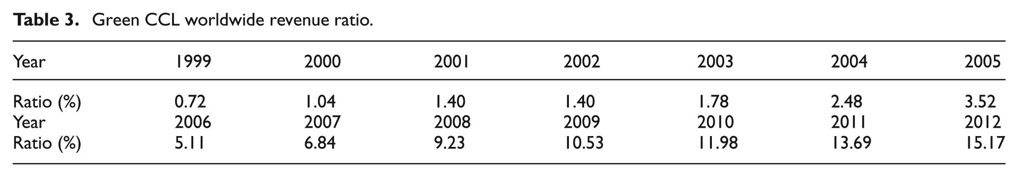
Printed circuit boards (PCBs) are crucial components of electric and electronic products that serve as a base connecting packaged components with their required electronic parts. Although PCBs have a significant role in linking the functional parts of an electronic product, they generate substantial pollution. Copper clad laminates (CCLs) are a core material of PCB production. To satisfy environmental requirements, CCL substrates are typically coated with non-halogen-based flame retardants to prevent flammability, thereby achieving environmental protection. Because of relevant environmental laws and regulations, the development of halogen-free PCB substrate material is an inevitable trend. After more than a decade of development, the revenue ratio of green halogen-free CCLs to worldwide CCL production increased continuously from 0.72% in 1999 to 3.52% in 2005, reaching 15.17% in 2012 (see Table 3). However, because the research and development (R&D) of green CCL is significantly challenging, CCL manufacturers must make substantial investments in the development of manufacturing equipment. In addition, the complex machining requirements of the PCB manufacturing process have prompted PCB manufacturers to increase investments in R&D resources and apply quality engineering approaches to identify optimum machining criteria. Therefore, forecasting growth trends in the production of green CCL materials is crucial for both PCB and CCL manufacturers. If the growth trends of green CCLs are clearly understood, relevant manufacturers can recognize trends earlier and thus gain a competitive advantage in the development of CCL technology and related markets. Forecasting the development of green products is an effective product sustainability life cycle assessment (SLCA) method. The SLCA approach enables organizations to define, assess, and communicate product sustainability.

Herbig et al. ¹ indicated that forecasting enables enterprises to predict unforeseen events or scenarios and provides managers with a basis for planning business operations; thus, forecasting is a highly crucial tool in business decision-making processes. The primary objective of this study was to forecast the growth trends of green electronic materials. Because the historical data samples of green electronic materials were limited and non-normally distributed, employing conventional regression analyses or time series methods for forecasting may be unsuitable for verifying relevant presumptions.

This study applied grey system theory as the forecasting method for several reasons. Grey system theory was employed because of its applicability to comprehensive analyses and observations of change in system development and subsequent long-term forecasting for system models with (a) incomplete information, (b) fuzzy behavioural patterns, or (c) unclear operating mechanisms. The core characteristic of grey system theory is that a forecasting model can be developed with few data records (as few as four), and numerous stringent assumptions regarding the sample population distribution are unnecessary.^2–11

Several researchers assert that the grey model(1,1) (GM(1,1)) offers high forecasting accuracy if the experimental sample data show a stable growth trend. If the sample data fluctuate significantly, the GM(1,1) requires modification to enhance the forecasting accuracy (e.g. the non-linear grey Bernoulli model (NGBM) and the Markov modification model).^12–16

Therefore, three grey forecasting models (i.e. the GM(1,1), NGBM(1,1), and grey Verhulst model) were adopted in this study for theoretical derivation and scientific verification. The results yielded by these methods were compared with the results of regression analysis to verify the forecasting accuracy and suitability of the three methods. The research conclusion and relevant suggestions were proposed based on the study results.

Literature review

Grey system theory

Grey system theory was introduced by Deng to conduct relational analysis and construction of a fuzzy system model with insufficient information, and investigate and understand the constructed system using prediction and decision-making methods. ¹⁷ In grey system theory, ‘black’, ‘white’, and ‘grey’ denote a complete lack of information, complete information, and insufficient or incomplete information, respectively. The theory was initially applied in the field of controls and has subsequently been adopted in numerous other fields, such as managerial decision-making, socio-economic research, and weather and hydraulic forecasting.

Grey system theory is especially effective for processing data that are uncertain, discrete, insufficient, or of multivariable inputs. Focusing on limited samples of uncertain data, grey system theory differs from the probability statistics used to investigate large samples with uncertainties and fuzzy theory that addresses cognitive uncertainty.^17–25

Previous research on grey system theory is summarized as follows: (a) grey generating techniques, (b) grey relational analysis, (c) grey model construction, (d) grey prediction, (e) grey decision-making, and (f) grey control.^{17–19,23–25}

In recent years, grey forecasting has been widely applied to management decision-making, socio-economic research, weather and water forecasting, and disaster prevention. For example, Yao et al. ²⁶ employed a modified grey forecasting model to predict electricity demand and obtained excellent forecasting outcomes. Hu used GM(1,1) to construct a forecasting model that enabled consumers intending to purchase a new car to make optimal choices. Consumers identified the optimal choice after inputting information of a specific brand, price, safety, function, and fuel consumption. ²⁷ Wang adopted a modified GM(1,1) to predict the number of tourists who visited Taiwan from Hong Kong, the United States, and Germany between 1989 and 2000. Research shows that the modified GM(1,1) yields high forecasting accuracy and reduces the cost and time required for data collection because the model does not require a large sample data set. ²⁸ Kayacan, Ulutas, and Kaynak employed the NGBM and grey Markov models to predict the Euro to USD exchange rates for 2005–2007. The results indicated that the models yielded high accuracy when the experimental sample data exhibited stable growth trends. ²⁹

Research methodology

GM(1,1) forecast modelling

The GM(1,1) is a first-order differential equation with one input variable and is used for prediction according to grey theory. Using GM(1,1), grey prediction is a forecasting approach that identifies the future dynamics of each term in a specific data sequence using available data. The advantage of GM(1,1) is that it necessitates limited data, and its mathematic operations are simple. Numerous types of grey predictions exist, including sequence, calamity, financial, and system predictions.^{2–4,12–14}

This study focuses specifically on sequence predictions. Sequence prediction directly constructs a grey prediction model using the data available. The procedure of grey prediction modelling based on GM(1,1) is explained in the following.

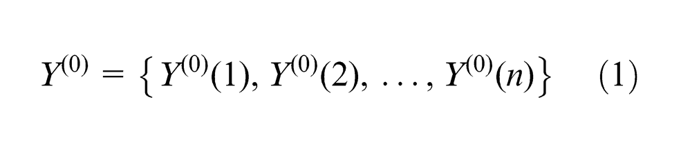
Grey prediction is based on the time series of GM(1,1) and can be derived as follows: Let Y be the dependent variable and X_i(I = 1, 2, 3, …, N− 1) be the explanatory variable and assume that the data are formed from period 1 to n, then the initial equation can be expressed as

$$Y^{(0)}=\{Y^{(0)}(1),Y^{(0)}(2),\dots ,Y^{(0)}(n)\}$$

(1)

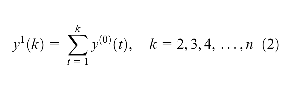
When this sequence undergoes accumulated generating operation (AGO) computations, the generated sequence y⁽¹⁾ can be obtained

$$y^1\left(k\right)=\sum _{t=1}^k{y}^{\left(0\right)}\left(t\right),k=2,3,4,\dots ,n$$

(2)

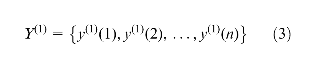
If y⁽¹⁾(1) = y⁽⁰⁾(1), then the generated sequence Y⁽¹⁾ is

$$Y^{(1)}=\{y^{(1)}(1),y^{(1)}(2),\dots ,y^{(1)}(n)\}$$

(3)

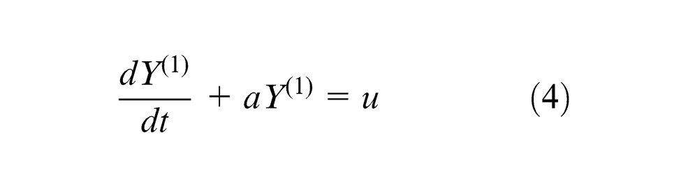
The differential equation of GM(1,1), which is a first-order and single-variable differential equation, for the sequence indicated by equation (3) is defined as follows (where u is a constant)

$$\frac{d{Y}^{(1)}}{\mathrm{dt}}+a{Y}^{(1)}=u$$

(4)

From the derivative definition

$$\frac{d{y}^{\left(1\right)}\left(t\right)}{\mathrm{dt}}=\underset{\Delta t\to 0}{lim}\frac{y^{(1)}(t+\Delta t)-y^{\left(1\right)}\left(t\right)}{\Delta t}$$

(5)

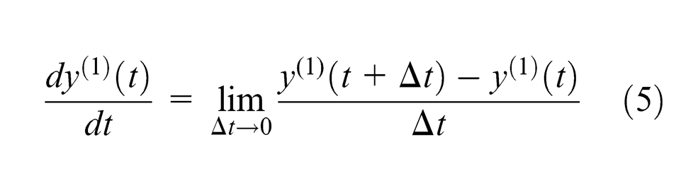
where equation (5) is a discrete dynamic system; therefore, assuming the interval period is uniform (i.e. $\Delta t=1$ ), the grey difference equation can be defined as

$$\frac{\Delta y^{\left(1\right)}(t)}{\Delta t}=y^{\left(1\right)}(k+1)-y^{\left(1\right)}(k)$$

(6)

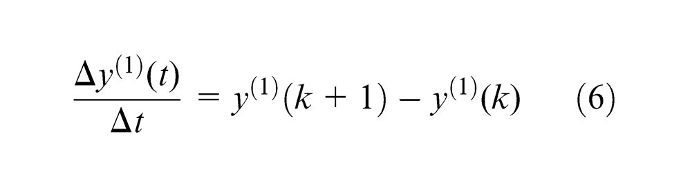
In grey theory, the background value of the rate of change $d{y}^{\left(1\right)}(t)/\mathrm{dt}$ is defined as the population related to $d{y}^{\left(1\right)}(t)/\mathrm{dt}$ , when $d{y}^{\left(1\right)}(t)/\mathrm{dt}$ ranges between y(t+Δt) and y(t−Δt). Generally, the linear centre of the range y(t+Δt) to y(t−Δt) can be adopted as the background value. Therefore, the relationship between the grey difference equation and its whitening equation can be expressed as

$$y^{(0)}(t)=y^{(1)}(t)-y^{(1)}(t-1)\approx \frac{d{y}^{(1)}(t)}{\mathrm{dt}}$$

(7)

$$Z^{(1)}(t)=\frac{1}{2}[y^{(1)}(t-1)+y^{(1)}(t)]\approx y^{(1)}(t)$$

(8)

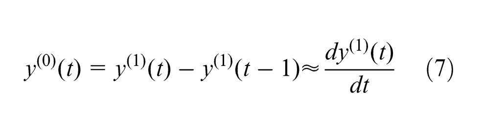
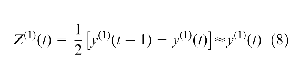
Substituting equations (7) and (8) into equation (6) provides

$$Y^{\left(0\right)}\left(t\right)+a{Z}^{\left(1\right)}\left(t\right)=u$$

(9)

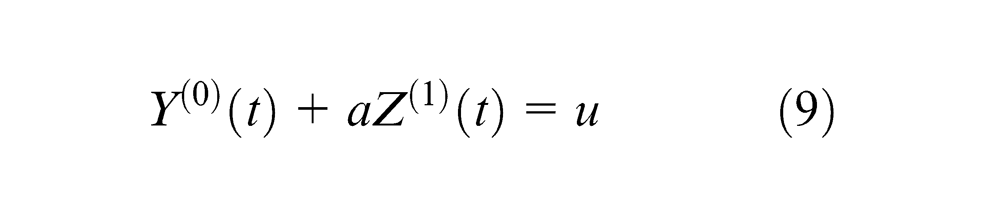
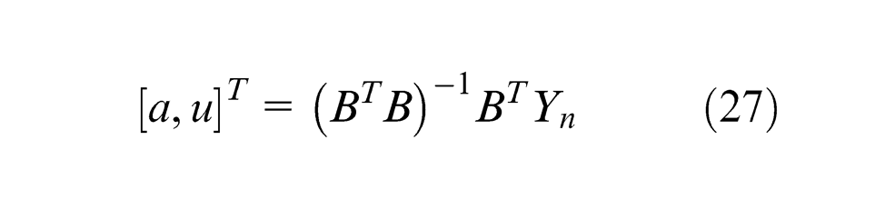
By applying the method of least squares, a and u can be calculated as follows

$${[a,u]}^T={(B^{T}B)}^{-1}{B}^{T}Y$$

(10)

$$Y={[Y^{(0)}(2),Y^{(0)}(3),\dots ,Y^{(0)}(n)]}^T$$

(11)

$$B_{(1,1)}=\left[\begin{array}{c}\hfill -\frac{1}{2}(Y^{(1)}(1)+Y^{(1)}(2)),1\hfill \\ \multicolumn{1}{c}{-\frac{1}{2}(Y^{(1)}(2)+Y^{(1)}(3)),1}\\ \multicolumn{1}{c}{⋮}\\ \multicolumn{1}{c}{-\frac{1}{2}(Y^{(1)}(n-1)+Y^{(1)}(n)),1}\end{array}\right]$$

(12)

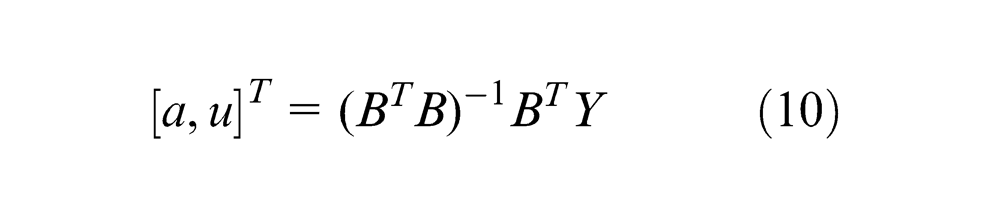
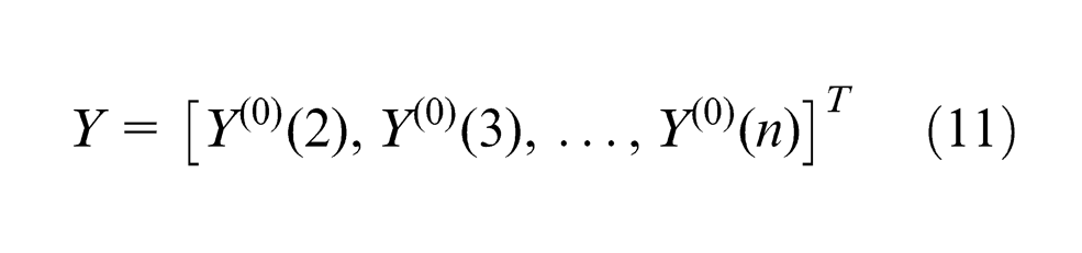
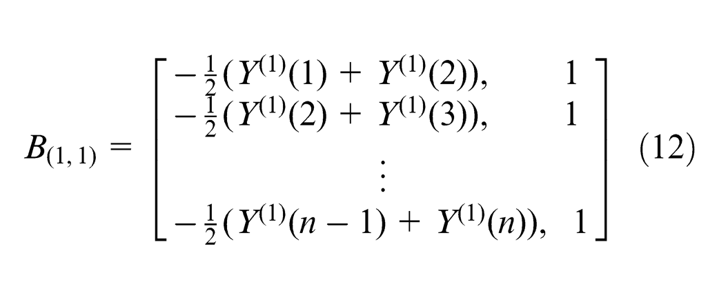
Substituting a and u from equation (10) into the discrete approximate equation obtained by solving equation (6), the grey AGO equation is obtained as follows

$${\hat{Y}}^{(1)}(k+1)=[Y^{\left(0\right)}\left(1\right)-\frac{u}{a}]e^{-\mathrm{ak}}+\frac{u}{a}$$

(13)

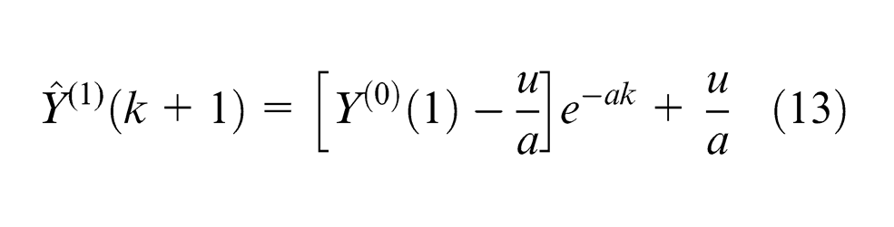
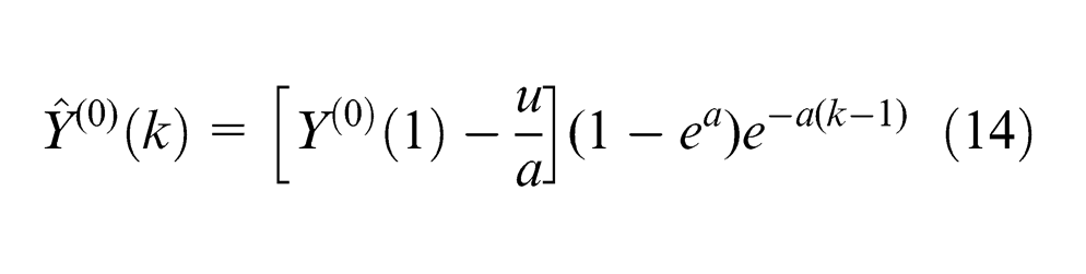
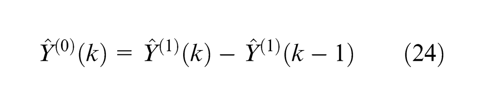
The inverse accumulated generating operation (IAGO) was then used to recover the equation and obtain the desired forecasting model as follows

$${\hat{Y}}^{(0)}\left(k\right)=[Y^{\left(0\right)}\left(1\right)-\frac{u}{a}](1-e^a)e^{-a(k-1)}$$

(14)

A posterior predictive check is required to verify the forecasting accuracy of GM(1,1), where the posterior ratio C and error frequency ratio p (defined below) are used to measure the forecasting accuracy.^12–14

The residual q⁽⁰⁾(k) is defined as

$$\begin{array}{cc}\multicolumn{1}{c}{}& q^{\left(0\right)}\left(k\right)=y^0\left(k\right)-{\hat{y}}^{\left(0\right)}\left(k\right),\text{where}k=2,3,4,\hfill \\ \multicolumn{1}{c}{}& q^{(0)}=[q^{(0)}(2),q^{(0)}(3),\dots ,q^{(0)}(n)]\hfill \end{array}$$

(15)

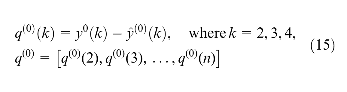
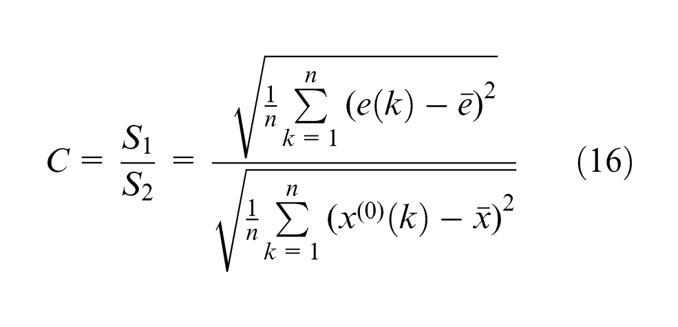
By assuming that S₁ is the standard deviation of residual q⁽⁰⁾(k) and S₂ is the standard deviation of the raw datum y⁽⁰⁾(k), the posterior ratio C is defined as

$$C=\frac{S_1}{S_2}=\frac{\sqrt{\frac{1}{n}\sum _{k=1}^n{(e\left(k\right)-\overline{e})}^2}}{\sqrt{\frac{1}{n}\sum _{k=1}^n{(x^{(0)}\left(k\right)-\overline{x})}^2}}$$

(16)

The error frequency ratio p is expressed as follows

$$p=\mathrm{prob}·\{|q^{(0)}(k)-\overline{q}|<0.6745S_2\}$$

(17)

where $\overline{q}$ is the mean of q⁽⁰⁾(k).

Assessment of the forecasting model accuracy is based on specific indicators for accuracy ranking, where a small C value indicates higher discreteness among raw data, and lower discreteness in the residual indicates a higher forecasting accuracy. A larger p value shows that the difference between the residual and the residual mean value is less than 0.6745, and that more S₂ data exist, indicating higher forecasting accuracy. Table 1 shows the forecasting accuracy rankings.

Table 1.

Grey prediction model accuracy ranking. ¹⁹

Level	P	C	Forecasting accuracy ranking
1	$⩾0.95$	$⩽0.35$	Good
2	$⩾0.80$	$⩽0.50$	Qualified
3	$⩾0.70$	$⩽0.65$	Average
4	$⩽0.70$	$⩾0.65$	Unqualified

NGBM

The NGBM is an original forecasting model that integrates the GM(1,1) with a Bernoulli differential equation. The NGBM retains the simple derivation process of the GM(1,1) and requires a sample size of 4, which reduces forecasting errors and improves the forecasting accuracy of the GM(1,1) for non-linear data.^{11–16,28,29}

The GM(1,1) is a special example of the NGBM. The derivation process for the NGBM was as follows:

1. First define the data obtained as the original series. A new series can be obtained through calculation with AGO. The first three calculation equations for the NGBM are identical to equations (1)–(3) for the GM(1,1).

2. The subsequent calculation equations for the NGBM differ from those for the GM(1,1). The Bernoulli equation was used to construct the NGBM differential/difference equations.

   The NGBM differential equation is given as follows

   $$\frac{d{Y}^{\left(1\right)}}{\mathrm{dt}}+a{Y}^{\left(1\right)}=u{\left[Y^{\left(1\right)}\right]}^r$$

   (18)

   Substituting equation (18) into equations (5)–(8) for the GM(1,1), NGBM differential equation can be expressed as follows

   $$Y^{\left(0\right)}\left(t\right)+a{Y}^{\left(1\right)}\left(t\right)=u{[Z^{\left(1\right)}(k)]}^r,t=2~n$$

   (19)

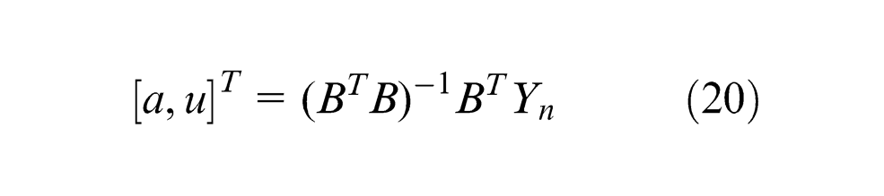
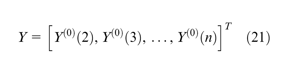
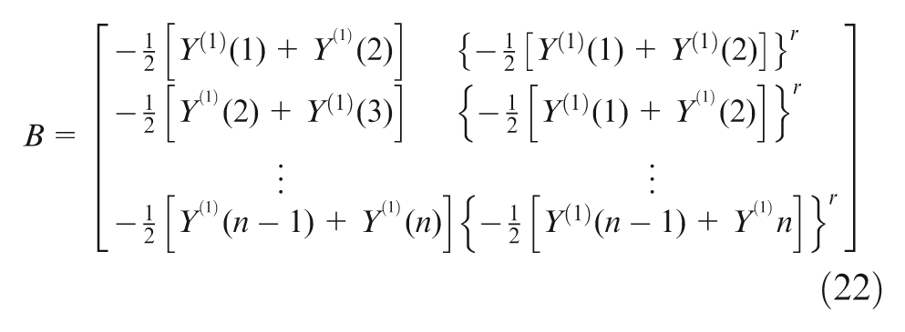
3. Use the least squares method, NGBM differential equation, and NGBM difference equation to obtain a and u

   $${[a,u]}^T={(B^{T}B)}^{-1}{B}^T{Y}_n$$

   (20)
   $$Y={[Y^{\left(0\right)}\left(2\right),Y^{\left(0\right)}\left(3\right),\dots ,Y^{\left(0\right)}\left(n\right)]}^T$$

   (21)
   $$B=\left[\begin{array}{c}\hfill -\frac{1}{2}[Y^{\left(1\right)}(1)+Y^{\left(1\right)}(2)]{\{-\frac{1}{2}[Y^{\left(1\right)}(1)+Y^{\left(1\right)}(2)]\}}^r\hfill \\ \multicolumn{1}{c}{-\frac{1}{2}[Y^{\left(1\right)}(2)+Y^{\left(1\right)}(3)]{\{-\frac{1}{2}[Y^{\left(1\right)}(1)+Y^{\left(1\right)}(2)]\}}^r}\\ \multicolumn{1}{c}{⋮⋮}\\ \multicolumn{1}{c}{-\frac{1}{2}[Y^{\left(1\right)}(n-1)+Y^{\left(1\right)}(n)]{\{-\frac{1}{2}[Y^{\left(1\right)}(n-1)+Y^{\left(1\right)}n]\}}^r}\end{array}\right]$$

   (22)

4. Use the grey differential equation to obtain the grey accumulated equation

   $$\begin{array}{cc}\multicolumn{1}{c}{{\hat{Y}}^{\left(1\right)}(k+1)}& ={[{[Y^{(0)}{(1)}^{(1-r)}-\frac{u}{a}]}^{e^{-a(1-r)k}}+\frac{u}{a}]}^{\left(\frac{1}{1-r}\right)},\hfill \\ \multicolumn{1}{c}{k=1~n}\end{array}$$

   (23)

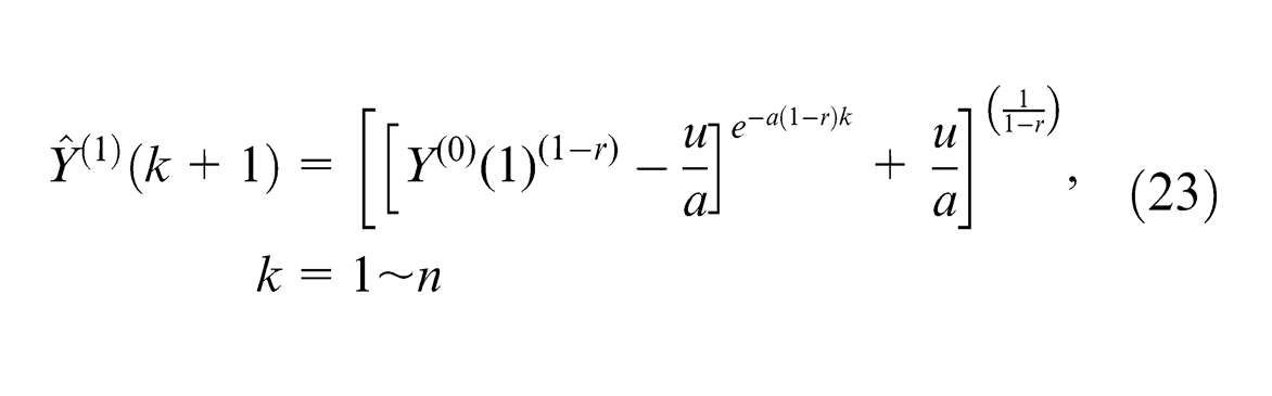
5. Use the IAGO to reduce equation (23) and obtain the demand forecasting model

   $${\hat{Y}}^{\left(0\right)}\left(k\right)={\hat{Y}}^{\left(1\right)}\left(k\right)-{\hat{Y}}^{\left(1\right)}(k-1)$$

   (24)

Grey Verhulst model

The characteristics of the grey Verhulst model and GM(1,1) are identical. An equation for limiting development is included in the GM(1,1). The grey Verhulst model is also a special example of the NGBM.^11–16 The derivation process for the grey Verhulst model was as follows:

1. First define the data obtained as the original series. A new series can be obtained through calculation using AGO. The first three calculation equations for the grey Verhulst model are identical to equations (1)–(3) for the GM(1,1).

2. Establish differential/difference equations for the grey Verhulst model.

   The grey Verhulst differential equation is given as

   $$\frac{d{Y}^{(1)}}{\mathrm{dt}}+a{Y}^{(1)}=u{\left[Y^{(1)}\right]}^2$$

   (25)

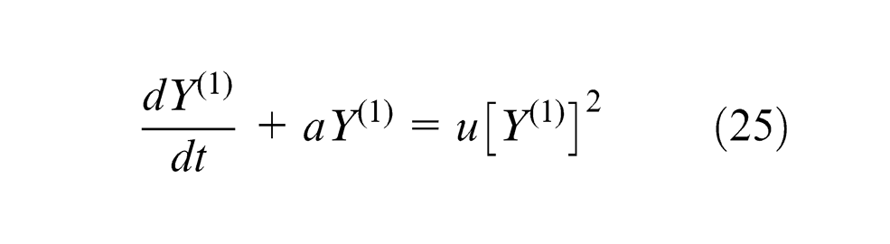
   By substituting equation (25) into equations (5)–(8) for the GM(1,1), an NGBM differential equation can be expressed as follows

   $$Y^{\left(0\right)}\left(t\right)+a{Y}^{\left(1\right)}\left(t\right)=u{[Z^{\left(1\right)}(k)]}^2,t=2~n$$

   (26)

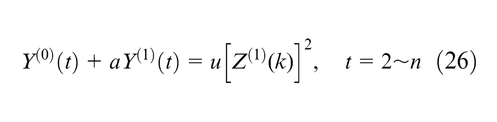
3. Use the least squares method, grey Verhulst differential equation, and grey Verhulst difference equation to determine a and u

   $${[a,u]}^T={\left(B^{T}B\right)}^{-1}{B}^T{Y}_n$$

   (27)
   $$Y={[Y^{\left(0\right)}\left(2\right),Y^{\left(0\right)}\left(3\right),\dots ,Y^{\left(0\right)}\left(n\right)]}^T$$

   (28)
   $$B=\left[\begin{array}{c}\hfill -\frac{1}{2}[Y^{\left(1\right)}(1)+Y^{\left(1\right)}(2)]{\{-\frac{1}{2}[Y^{\left(1\right)}(1)+Y^{\left(1\right)}(2)]\}}^2\hfill \\ \multicolumn{1}{c}{-\frac{1}{2}[Y^{\left(1\right)}(2)+Y^{\left(1\right)}(3)]{\{-\frac{1}{2}[Y^{\left(1\right)}(1)+Y^{\left(1\right)}(2)]\}}^2}\\ \multicolumn{1}{c}{⋮⋮}\\ \multicolumn{1}{c}{-\frac{1}{2}[Y^{\left(1\right)}(n-1)+Y^{\left(1\right)}(n)]{\{-\frac{1}{2}[Y^{\left(1\right)}(n-1)+Y^{\left(1\right)}n]\}}^2}\end{array}\right]$$

   (29)

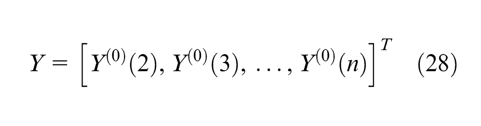
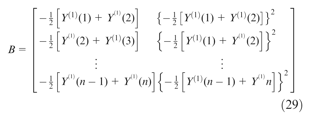
4. Use the grey differential equation to obtain the grey accumulated equation

   $$\begin{array}{cc}\multicolumn{1}{c}{{\hat{Y}}^{\left(1\right)}(k+1)}& ={[{[Y^{(0)}{(1)}^{(-1)}-\frac{u}{a}]}^{e^{\mathrm{ak}}}+\frac{u}{a}]}^{(-1)},\hfill \\ \multicolumn{1}{c}{k=1~n}& \hfill \end{array}$$

   (30)

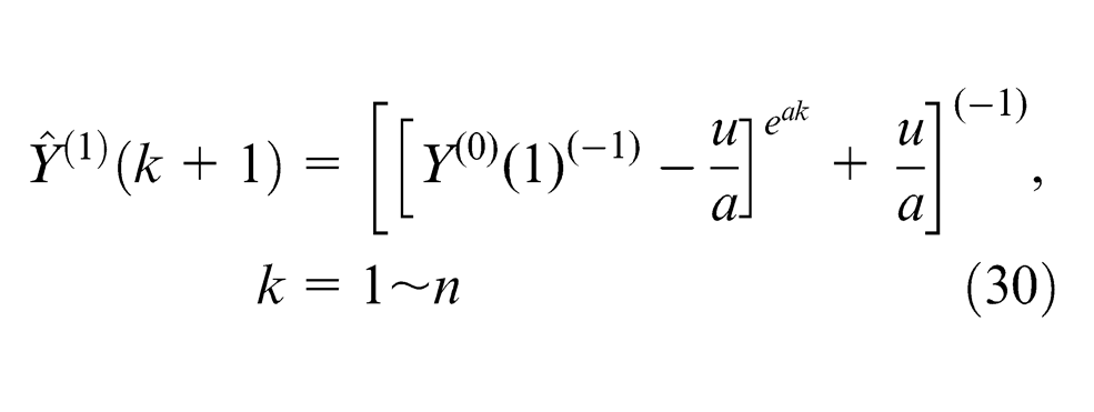
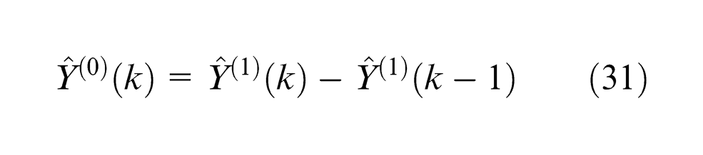
5. Reduce equation (30) using the IAGO to obtain the demand forecasting model

   $${\hat{Y}}^{\left(0\right)}\left(k\right)={\hat{Y}}^{\left(1\right)}\left(k\right)-{\hat{Y}}^{\left(1\right)}(k-1)$$

   (31)

Evaluation of forecasting accuracy

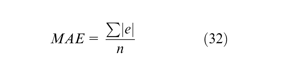
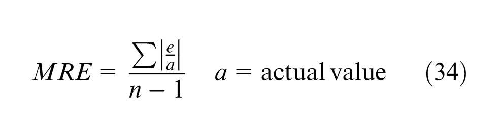
The difference between an actual value and a predicted value obtained from a forecasting model is considered the forecasting error, which determines the success or failure of a forecasting model. This study adopted four commonly used evaluation methods, namely, mean absolute error (MAE), mean squared error (MSE), mean relative error (MRE), and mean absolute percentage error (MAPE). This study used these four methods to examine the accuracy of a forecasting model.^12,30,31

Each error type was defined as follows:

1. MAE – a small MAE value indicates good forecasting accuracy

   $$\mathrm{MAE}=\frac{\sum \left|e\right|}{n}$$

   (32)

2. MSE – a small MSE value indicates good forecasting accuracy

   $$\mathrm{MSE}=\frac{\sum e^2}{n-1}$$

   (33)

3. MRE – a small MRE value indicates good forecasting accuracy

   $$\mathrm{MRE}=\frac{\sum \left|\frac{e}{a}\right|}{n-1}a=\text{actual value}$$

   (34)

4. MAPE – a small MAPE value indicates good forecasting accuracy

   $$\mathrm{MAPE}=\frac{\sum \left|\frac{e}{a}\right|}{n}\times 100\%a=\text{actual value}$$

   (35)

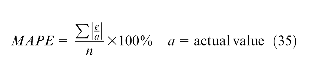
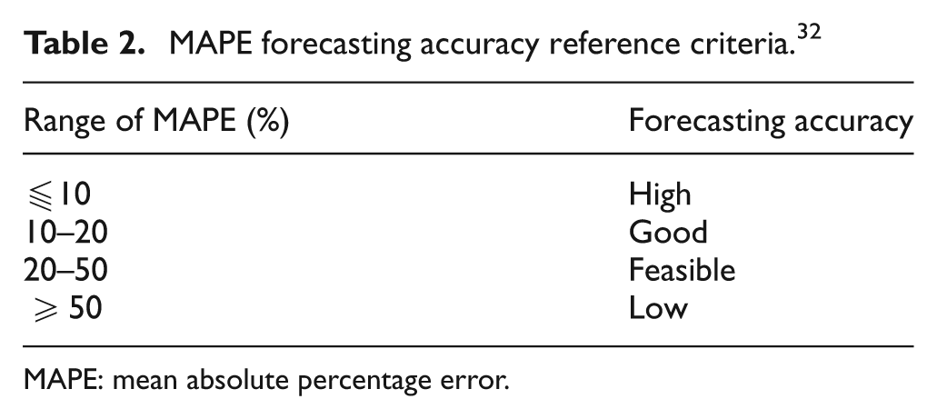
A small error value denotes high accuracy. According to Lewis, an MAPE value of less than 10% indicates high forecasting accuracy (Table 2). ³²

Table 2.

MAPE forecasting accuracy reference criteria. ³²

Range of MAPE (%)	Forecasting accuracy
$⩽10$	High
10–20	Good
20–50	Feasible
≥50	Low

MAPE: mean absolute percentage error.

Results and discussion

Research data and calculation processes

CCL production involves using a fibreglass cloth or any reinforcing material impregnated with resin and coated with single- or double-sided copper foil that undergoes hot pressing under high pressures. To achieve environmental protection, CCLs are typically coated with non-halogen-based flame retardants to prevent flammability and produce an environmentally friendly material. With development over the last decade, the revenue ratio of green halogen-free CCLs to worldwide CCL yield has increased consistently. According to CCL market statistics published by Prismark, the revenue ratio of green CCLs increased from 0.72% in 1999 to 3.52% in 2005, reaching 15.17% in 2012 (records for the 14 years are listed in Table 3).

Table 3.

Green CCL worldwide revenue ratio.

Year	1999	2000	2001	2002	2003	2004	2005
Ratio (%)	0.72	1.04	1.40	1.40	1.78	2.48	3.52
Year	2006	2007	2008	2009	2010	2011	2012
Ratio (%)	5.11	6.84	9.23	10.53	11.98	13.69	15.17

Using the original data shown in Table 3, this study adopted three grey forecasting models (i.e. the GM(1,1), NGBM(1,1), and grey Verhulst model) for theoretical derivation and scientific verification. The results yielded by these methods were compared with the results of regression analysis to verify the forecasting accuracy and suitability of the three methods. The calculation processes are shown in Figure 1.

Figure 1.

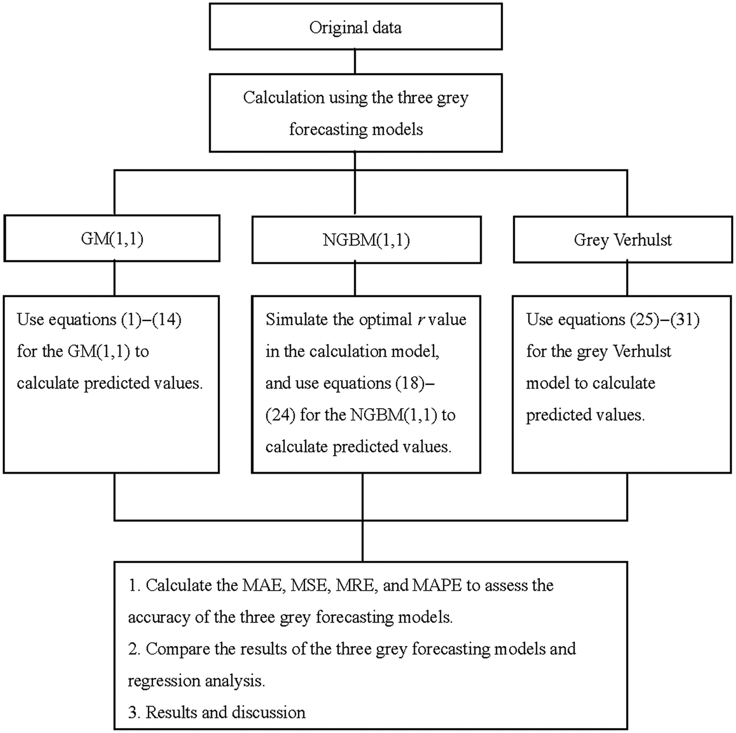
Calculation processes and framework.

GM(1,1) results

The GM(1,1) was established with a sample size of 4. A MATLAB program was used to calculate the predicted values according to equations (1)–(14). The predicted values of the green material ratio were calculated as 1.66% for 2003, 1.96% for 2004, and 3.21% for 2005. Further details are provided in Table 4. The predicted values for 2013, 2014, and 2015 were 16.77%, 18.72%, and 20.48%, respectively.

Table 4.

Predicted values obtained from the four forecasting models (%).

Year	Revenue ratio of halogen-free substrate material to substrate material (%)	GM(1,1)-predicted values	NGBM(1,1)-predicted values	Grey Verhulst–predicted value	Regression analysis–predicted value
1999	0.72
2000	1.04
2001	1.40				0.18
2002	1.40				1.36
2003	1.78	1.66	1.73	1.75	2.55
2004	2.48	1.96	2.36	2.38	3.73
2005	3.52	3.21	3.47	3.59	4.91
2006	5.11	4.78	4.85	5.02	6.09
2007	6.84	7.04	7.06	7.17	7.27
2008	9.23	9.22	9.30	9.42	8.46
2009	10.53	12.08	12.11	12.19	9.64
2010	11.98	13.00	13.05	13.14	10.82
2011	13.69	13.57	13.66	13.76	12
2012	15.17	15.03	15.12	15.28	13.18
2013		16.77	16.84	16.90	14.37
2014		18.72	18.88	18.95	15.55
2015		20.48	20.57	20.63	16.73

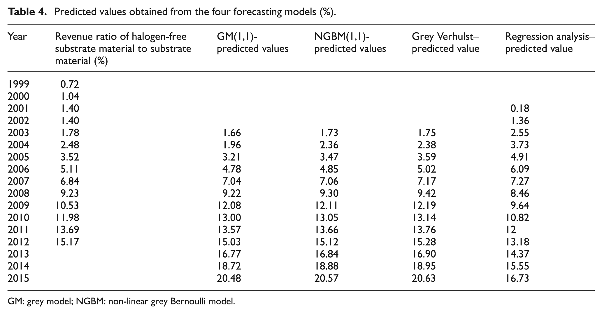
GM: grey model; NGBM: non-linear grey Bernoulli model.

Equations (16) and (17) were used to calculate the posterior ratio C and the error frequency P. As shown in Table 3, the C value obtained from the model was 0.09 ( $⩽0.35$ ), indicating that the model forecasting accuracy was rated as ‘good’, which was the top-level rating. The P value was 0.70 ( $⩾0.70$ ), indicating that the model forecasting accuracy was rated as ‘just’, which was the third-level rating.

The forecasting accuracy indicators for the GM(1,1) were obtained according to equations (32)–(35) using an Excel program; the values were 0.432 for MAE, 0.445 for MSE, 0.079 for MRE, and 7.104% for MAPE. Detailed information is provided in Table 5.

Table 5.

Forecasting accuracy indicators for the four forecasting models.

Forecasting accuracy indicator for model	GM(1,1)	NGBM(1,1)	Grey Verhulst	Regression analysis
C	0.09	0.07	0.07	–
P	0.70	0.99	0.96	–
MAE	0.432	0.350	0.381	1.132
MSE	0.445	0.421	0.476	1.642
MRE	0.079	0.047	0.048	0.234
MAPE	7.104%	4.262%	4.303%	21.055%

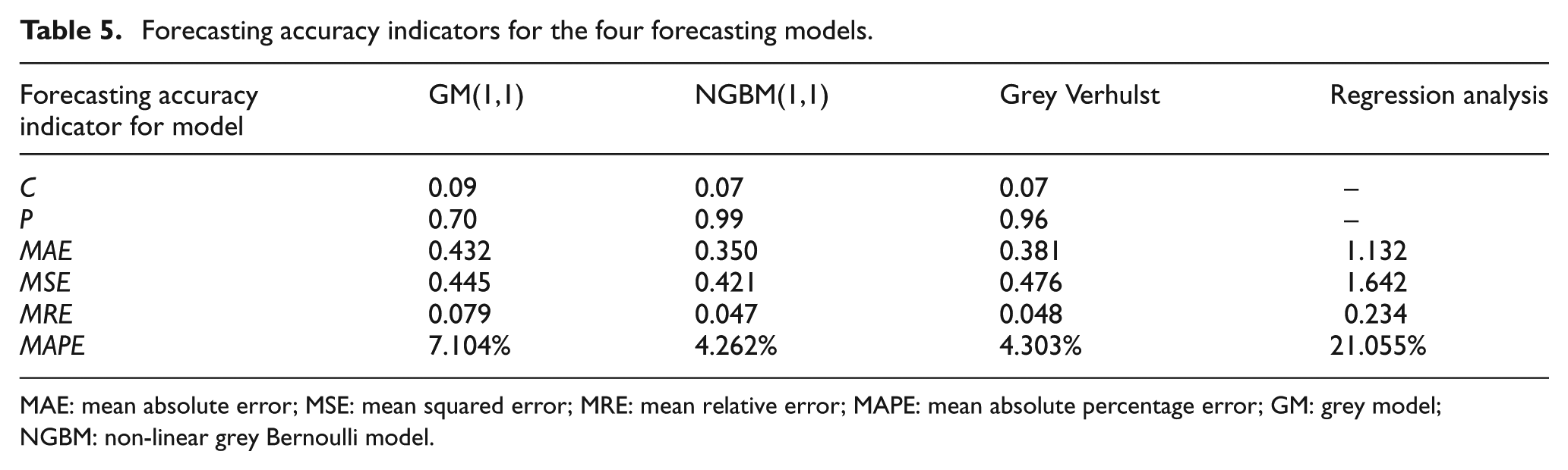
MAE: mean absolute error; MSE: mean squared error; MRE: mean relative error; MAPE: mean absolute percentage error; GM: grey model; NGBM: non-linear grey Bernoulli model.

NGBM(1,1) results

For the NGBM(1,1), a MATLAB program was used to calculate the predicted values according to equations (18)–(24). The predicted values of the green material ratio were calculated as 1.73% for 2003, 2.36% for 2004, and 3.47% for 2005. Further details are provided in Table 4. The predicted values for 2013, 2014, and 2015 were 16.84%, 18.88%, and 20.57%, respectively.

The C value obtained from this model was 0.07 ( $⩽0.35$ ), indicating that the model forecasting accuracy was rated as ‘good’, which was the top-level rating. The P value was 0.99 ( $⩾0.95$ ), indicating that the model forecasting accuracy achieved the top-level rating ‘good’.

The forecasting accuracy indicators for the NGBM(1,1) were obtained from equations (32)–(35) using an Excel program; the values were 0.350 for MAE, 0.421 for MSE, 0.047 for MRE, and 4.262% for MAPE. Detailed information is provided in Table 5.

Grey Verhulst model results

The grey Verhulst model was established, and a MATLAB program was used to calculate the predicted values according to equations (25)–(31). The predicted values of the green material ratio were calculated as 1.75% for 2003, 2.38% for 2004, and 3.59% for 2005. Further details are provided in Table 4. The predicted values for 2013, 2014, and 2015 were 16.90%, 18.95%, and 20.63%, respectively.

The C value obtained from this model was 0.07 ( $⩽0.35$ ), indicating that the model forecasting accuracy was rated as ‘good’, which was the top-level rating. The P value was 0.96 ( $⩾0.95$ ), indicating that the model forecasting accuracy achieved the top-level rating ‘good’.

The forecasting accuracy indicators for the grey Verhulst model were obtained according to equations (32)–(35) using an Excel program; the values were 0.381 for MAE, 0.476 for MSE, 0.048 for MRE, and 4.303% for MAPE. Detailed information is provided in Table 5.

Regression analysis results

This study employed three grey forecasting models (i.e. the GM(1,1), NGBM(1,1), and grey Verhulst model) to forecast green material trends. To compare the forecasting accuracy of various methods, regression analysis was performed to forecast the trends for green materials, and the results were compared with those of the three methods mentioned previously.

With the data from 1999 to 2012, as shown in Table 3, the Minitab software program was used to construct a regression analysis model and scatter diagram. Detailed information is provided in Table 4 and Figure 2. The R₂ value for the model was 0.93, and the adjusted R² value was 0.93. The predicted values for 2013, 2014, and 2015 were 14.37%, 15.55%, and 16.73%, respectively. The regression equation is expressed as

$$\text{y}=1.1182\text{x}-2365$$

(35)

Figure 2.

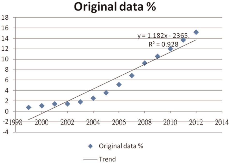
Regression analysis and scatter diagram.

The forecasting accuracy indicators were calculated according to equations (32)–(35) using an Excel program; the values were 1.132 for MAE, 1.642 for MSE, 0.234 for MRE, and 21.055% for MAPE. Detailed information is provided in Table 5.

Discussion

The forecasting accuracy of the three grey forecasting models was compared. Examining the values of the posterior ratio C and error frequency P (Table 5) in grey theory, the results showed that the forecasting accuracy of the NGBM(1,1) and grey Verhulst model was higher than that of the GM(1,1). According to the research results, the modified NGBM(1,1) and grey Verhulst model possessed superior forecasting capabilities compared to the original GM(1,1).

The forecasting accuracy of the three grey forecasting models was compared with that of the regression analysis model. According to the four accuracy indicators (i.e. MAE, MSE, MRE, and MAPE), no significant difference in forecasting accuracy existed between the NGBM(1,1) and grey Verhulst model. The NGBM(1,1) and grey Verhulst model offered the highest forecasting accuracy, followed by the GM(1,1). The regression analysis model yielded the lowest forecasting accuracy, as shown in Table 5.

In addition, according to Lewis, an MAPE value of less than 10% indicates high forecasting accuracy. ³² The MAPE value for the NGBM(1,1), grey Verhulst model, and GM(1,1) was 4.262%, 4.303%, and 7.104%, respectively; these values indicated that the three models yielded high forecast accuracy. The MAPE value for the regression analysis model was 21.055%, indicating feasible forecasting accuracy. Therefore, the regression analysis model yielded the lowest forecasting accuracy.

As shown in Figure 3, the predicted values obtained from the four forecasting models were compared with the actual values. The NGBM(1,1) provided the highest forecasting accuracy, followed by the grey Verhulst model and then the GM(1,1). The regression analysis model provided the lowest forecasting accuracy.

Figure 3.

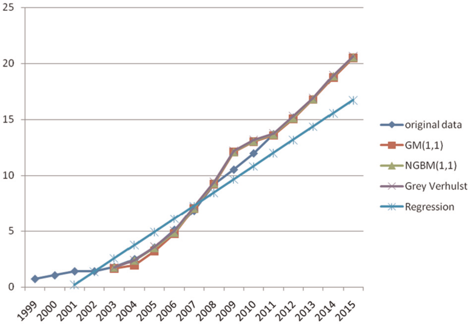
Comparison of the forecasting models.

Conclusion

The fundamental principles relevant to green materials are to design and develop low-pollution materials that generate minimal environmental pollution, to innovate and improve low-pollution manufacturing processes, and to recycle and reuse materials. The core materials of PCBs are CCLs. CCL substrates are coated with non-halogen-based flame retardants to prevent flammability and achieve environmental protection. Because laws and regulations related to environmental protection have been established, the design and development of halogen-free PCB substrate material is an inevitable trend. The R&D of green CCLs involves challenging technologies. Therefore, CCL manufacturers must make substantial investments in manufacturing equipment for developing green CCLs. In addition, the use of green CCLs in PCB fabrication and machining is complex and challenging; thus, PCB manufacturers must invest additional R&D resources and apply a quality engineering approach to identify the optimal machining methods. Consequently, forecasting the growth trends of green CCL materials is crucial for both PCB and CCL manufacturers. The revenue ratio of green CCLs to worldwide CCL production was approximately 15.17% in 2012. This study estimates that the revenue ratio of green CCLs to worldwide CCL production will be approximately 20.60% in 2015. To respond to this growth trend, CCL and PCB manufacturers must invest R&D resources in green CCL development.

The purpose of forecasting is to predict future events or situations that enterprises cannot control and provide a foundation for administrators to develop plans. Therefore, forecasting is critical for decision-making. The main purpose of this study was to forecast the growth trends of green electronic materials. However, the industry sample investigated in this study only numbered 14. Because of the limited samples of historical data, the data distribution did not exhibit a normal distribution pattern. Prediction methods for large data sets (e.g. conventional regression analysis, neural networks, and genetic algorithms) were not suitable for this study. Thus, three grey forecasting models (i.e. the GM(1,1), NGBM(1,1), and grey Verhulst model) were adopted for theoretical derivation and scientific verification. The results yielded by these methods were compared with the results of regression analysis to verify the forecasting accuracy and suitability of the three methods.

Based on the scientific evidence obtained in this study, the forecasting accuracy of the three grey forecasting models was compared with that of the regression analysis model. According to the four accuracy indicators (i.e. MAE, MSE, MRE, and MAPE), no significant difference in forecasting accuracy existed between the NGBM(1,1) and grey Verhulst model, which provided the highest forecasting accuracy, followed by that of the GM(1,1). The regression analysis model yielded the lowest forecasting accuracy. As confirmed in this study, for small data sets, the forecasting accuracy of the modified NGBM(1,1) and grey Verhulst model was higher than that of the original GM(1,1) and the regression analysis method.

The study results also show that the MAPE value for the NGBM(1,1), grey Verhulst, and GM(1,1) models was 4.262%, 4.303%, and 7.104, respectively. These three models showed high forecasting accuracy for small data sets. The MAPE value for the regression analysis model was 21.055, indicating feasible forecasting accuracy. Thus, the regression analysis model yielded the lowest forecasting accuracy.

This study adopted three grey forecasting models, and the research results demonstrate several advantages of grey forecasting: (a) grey forecasting does not require large historical data sets. The sample data size for grey forecasting can be determined according to actual situations and requirements. Generally, a minimum sample size of 4 is sufficient to construct a forecasting model. (b) Grey forecasting methods involve simple calculations. (c) Grey forecasting does not require numerous correlation factors and sample data can be obtained easily, substantially reducing the time and costs required for data collection. (d) Grey forecasting yields high forecasting accuracy. Previously, numerous industrial studies did not provide accurate predictions because of difficulties in collecting large-scale historical data. The authors suggest that subsequent researchers conduct follow-up investigations based on this study using different industries or adopt alternative research methods to perform comparative examinations. However, if the research targets require large data sets, and a large-scale sample survey must be conducted to collect sufficient amounts of information for data analysis, the authors recommend using conventional forecasting methods for such research.