
Abstract
An intelligent offline optimisation system for feed and spindle speed in three-axis machining of sculptured surfaces is presented. Optimisation is performed by a standard genetic algorithm seeking, in this instance, to minimise machining force variation along designated sections of the tool path. Machining force is modelled realistically, rather than mechanistically, by dedicated artificial neural networks trained with a low number of experimental data that are obtained from the very equipment on which machining is to be carried out. The artificial neural networks employ the material volume removed per tool revolution as calculated using a standard solid modelling engine. The artificial neural network model architecture is optimally determined in a rigorous way as opposed to often followed trial-and-error approaches, and it is made use of directly in the evaluation function of the optimiser. This framework is flexible enough to enable definition of constraints, additional evaluation criteria and desirable force patterns to guide optimisation. Effectiveness of the approach is successfully demonstrated for finish machining a hemispherical part.
Keywords
Introduction
Feed and spindle speed in current machining practice are selected conservatively often relying on experience in order to satisfy quality characteristics of the hemispherical part and at the same time to keep machining time as less as possible. 1 In sculptured surface machining, due to complex geometry and constantly varying cutting tool engagement, and thus material removal volume, feed and speed may need to be constantly varying too, to achieve dimensional and surface accuracy. 2 Such quality characteristics may be predicted indirectly through observation of the cutting force using a theoretical approach 3 or statistical/neural network approximations, expressing the relationship between the quality characteristic of interest and the machining parameters that affect it. The latter approach is well established in the case of 2-1/2-D milling where machining parameters are uniform4,5 but not in the case of free-form surfaces in the presence of scallops and regions with sharp inclination. 6
It becomes obvious that in complex machining cases where tool engagement varies constantly, optimisation of feed and spindle speed along the tool path is necessary. This should take into account the peculiarities of the equipment used and involve as few experiments as possible. Most machining optimisation work has been focusing on feed, employing the term ‘feed scheduling’, whereas spindle speed has been largely neglected or kept to the highest possible value following cutting tool manufacturers tables. 1 Note that feed per tooth directly determines instantaneous chip load, that is, machining forces, but is inversely proportional to spindle speed and proportional to feed. Therefore, both feed and spindle speed should be optimised at the same time. The current work aims to provide a solution to this problem.
Feed scheduling based on material removal rate (MRR) neglecting other factors (notably cutting forces and acceleration/deceleration constraints) has been shown to often result in excessively high feed rates.7,8 However, most commercial computer-aided manufacturing (CAM) software packages support it, due to computer numerical control (CNC) verification models that are already built into them. Feed scheduling based on machining forces has attracted a lot of research attention recently. The core of any such approach consists of accuracy in force prediction, which depends on accuracy of calculation of tool axial and radial engagement, and is trivial in 2.5-D pocket machining, 9 but perplexed in free-form surface machining. The latter case is dealt with a so-called mechanistic model involving chip dimension calculation and cutting force coefficients. To calculate chip dimensions, various techniques are used, including Boolean operations on tool–workpiece solid models in terms of either discretised slices 10 or volume swept by the cutting edges,11,12 z-maps, 13 point and curve-based discretisation methods,14,15 geometric analysis at any feed direction, 16 octrees 17 and dexels. 18 To determine cutting force coefficients, some experiments are always involved.19,20
Feed optimisation strategy may be simple, involving adjustment to keep force constant all along the tool path, 12 but other criteria can be used as an alternative or as a supplement as well as constraints. Such criteria involve chip volume per tooth 13 and MRR-based prediction of cutting force.17,21 Constraints may involve tool health and machine tool capabilities differentiated for roughing, semi-finishing and finishing stages, 22 contour error and the characteristics of the acceleration/deceleration profile of the feed drive systems. 23 Feed optimisation may be also combined with process control fed by a knowledge base of materials, machines and tools. 24
Optimisation of feed together with speed is less conspicuous in the literature. Merdol and Altintas 10 use a conventional constraint-based optimisation scheme involving both speed and feed to maximise MRR under various constraints. It seems that intelligent computation techniques can provide a solution to these more complex optimisation cases with particular focus on genetic algorithms (GAs) and other evolutionary algorithms. 25 Ip 26 was among the first to suggest MRR-based feed and speed optimisation under tool life and surface slope constraints using fuzzy logic, reaching relatively acceptable results but very fast. Artificial neural networks (ANNs) have been used to model cutting force as needed by a particle swarm optimisation (PSO) algorithm tackling both feed and speed under a comprehensive set of constraints, but results were demonstrated just for plain pocket milling. 27 Recently, ANNs, fuzzy logic and PSO were combined in modelling and adaptively controlling ball-end milling, in which case, offline optimisation formed the front-end of the system and a neural identifier captured process dynamics. 28
The view adopted in this work is that machining parameters and resulting quality in free-form machining are difficult to predict explicitly due to continuously varying tool engagement, the influence of machine tool system dynamics and current equipment status, for example, tool wear. Most of these factors are reflected in some way or another onto machining forces, which can effectively define optimisation criteria. ANNs have the potential to reflect machining force reality if trained with real data. Furthermore, optimisation flexibility is necessary in terms of configuring criteria and adding constraints. For instance, force constancy may need to be replaced by a particular force variation pattern desired, while feed variation may need to be limited, or feed variation may be preferred to speed variation and so on. GAs seem to be able to cover these optimisation requirements, with the additional advantage that the offline optimisation approach adopted does not impose any strict performance demands, certainly nothing close to those required by real-time optimisation systems.
The feed–speed optimisation system presented offers both realism in cutting force modelling and flexibility in optimisation setup, which constitute its contribution to current state of the art. The system is targeted at sculptured surface machining. Note that no specific theory relating to sculptured surfaces in particular needs to be employed because all volume removal calculations rely on Boolean operations along a short-feed movement distance corresponding to a fraction of a revolution of the cutting tool. Note also that for demonstration purposes, the finishing stage is examined, in which forces are generally low compared to the roughing stage but force variation is prominent due to scallop height variability induced by the latter. Section ‘The approach followed’ outlines the approach followed. Section ‘Volume of material removed per revolution’ presents calculation of machined volume, and section ‘Force model creation’ describes construction of the force model through an ANN. Section ‘Feed and speed optimisation’ presents feed and speed optimisation through a GA, and indicative results are given and discussed in section ‘Results and discussion’. Section ‘Conclusions and further work’ articulates the main findings and points to future research.
The approach followed
The approach adopted is depicted in Figure 1. It consists of two parts: (1) calculation of the cutting force at a sufficient number of points along the tool path and (2) manipulation of the cutting force at these points through offline optimisation of tool feed and speed.
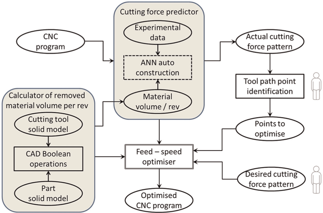
Overall approach.
Cutting force calculation
The cutting force is computed by an ANN. This was decided, as opposed to deploying analytical or numerical models because the latter would be, in the general case, inaccurate as they need to be based on basic assumptions. Such assumptions usually neglect specific properties of the machine tool, such as its dynamics, geometric accuracy and so on; of the cutting tool, such as interface properties, geometric accuracy and so on; and even of the actual workpiece material. An ANN, by contrast, can be trained with data stemming from the very equipment and material at hand and can be retrained if any changes occur.
The main issue is to select as input parameters those that really affect the cutting process. Feed and cutting speed should obviously be two of the inputs since they are directly involved in cutting mechanics and in addition, they constitute the only free parameters. Furthermore, cutting force varies due to shape complexity of sculptured surface parts. For given speed and feed, the material volume removed per revolution determines the resistance that the tool encounters along its path, that is, the cutting force. Material removal volume variation is due to cutting tool engagement variation with the part, which is due to complex geometry of the latter. Thus, material volume removed per cutting tool revolution is a suitable input to the ANN capturing this behaviour described above. The ANN has just one output, that is, the cutting force.
Two steps are executed for establishing the ANN model of the cutting force:
Designing of experiments (DoEs) and executing the planned experiments for ANN-related data acquisition. The cutting force values in each example fed into the ANN in the training process need to be measured experimentally on the same equipment intended for the actual machining of the part. To this end, a DoE exercise is conducted so as to minimise the number of required training examples. Cutting force is measured using a piezoelectric dynamometer. Details on DoE are given in Montgomery. 29
Determining optimum ANN architecture and – at the same time – using it for training. The main disadvantage of the ANN approach for cutting force modelling is the lack of a theoretical basis for automated architecture development which has very often been handled by trial and error. In this work, a methodology for determining the optimum architecture of the ANN was adopted using novel criteria for assessing quality of the ANN favouring, besides performance, structural simplicity.
Once the ANN is trained, the following steps are executed for calculating the cutting force:
Determining the coordinates of the particular point(s) from the CNC tool path. Interpolation is necessary that computes equidistant point coordinates along the tool path based on the pertinent G-code commands, that is, standardised linear and circular and possibly non-standard spline commands.
Calculating material removal volume per revolution for the particular point(s). This is achieved by using three-dimensional (3D) solid models of both the part and the tool and Boolean operations.
Executing the ANN for given feed, speed and volume removed per tool revolution.
Cutting force manipulation
Once cutting force is known along the tool path, it is relatively easy to recognise the regions in which its magnitude and/or variation need manipulation. In general, manipulation of the cutting force may mean not just reducing its magnitude but also smoothing out its variations or generally forcing it to follow a predetermined pattern. This is based on changing the feed and/or speed. Note, however, that there are practically a large number of combinations of speed and feed values that yield the same cutting force.
Thus, a GA is advocated that will seek an optimum combination of feed and speed at every point along the tool path region of interest so as to achieve the desired effect on the cutting force. Thus, the GA makes use of the ANN developed to calculate cutting force in order to evaluate possible feed–speed solutions given the material volume removed per revolution of the cutter, which is fixed for each point since the tool path is also fixed. Evaluation of the solution is dependent upon the particular criteria adopted concerning the cutting force, as expressed in the pertinent cost function, for instance, keeping cutting force constant or smoothening force variations or following a desired pattern, within applicable constraints usually referring to the minimum/maximum force or its derivative (variation step).
Volume of material removed per revolution
The volume of part material that is removed in each revolution of the cutting tool is calculated using Boolean operators. Within the time interval within which the tool completes one rotation, it is also fed through a distance corresponding to the applicable feed. This is done in sufficiently small steps along the tool path. At each position, a Boolean intersection between the tool and the part is executed. The total volume removed is the sum of the individual intersection volumes corresponding to the time that a full rotation takes with good accuracy. A Boolean subtraction updates the part thereby performing volume removal. All commercially available computer-aided design (CAD) solid modellers are capable of performing this calculation since Boolean operations and mass property calculation functions are universally implemented. In order to implement volume removal calculation, the part’s solid model is necessary; this may be the initial form of the workpiece in the case of rough machining or a roughed shape in the case of finish machining, often obtained by simulating the roughing stage on a CAM system and expressed in STL format. The cutting tool’s solid model is also needed. Parametric modelling serves the purpose better. For instance, a ball-end mill with two cutting edges was parametrically modelled (see Figure 2(a)), the main parameters being diameter, helix angle and axial and radial rake angle.
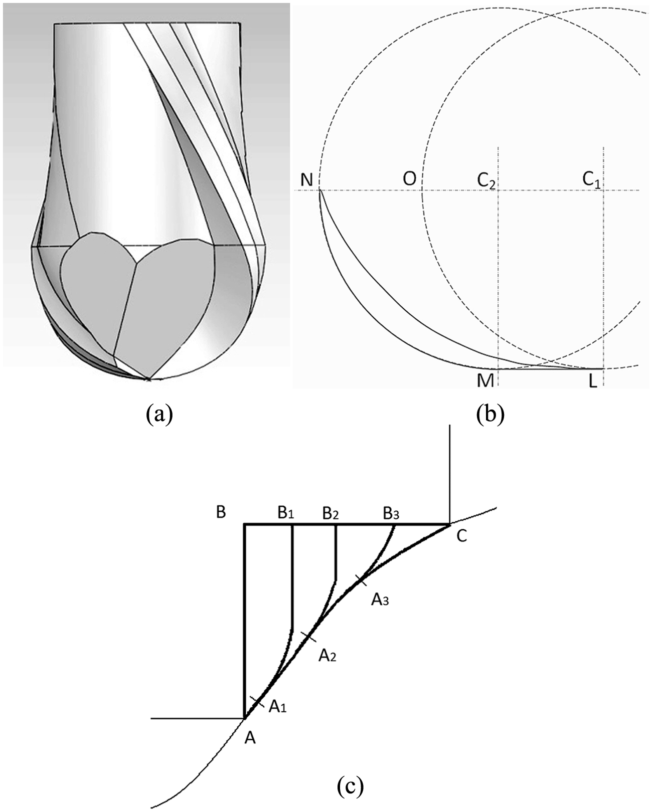
Volume removal calculation through Boolean operations: (a) parametric solid model of a two-fluted ball-end mill, (b) chip cross-section overestimate (area LMNOL instead of LNOL) on a horizontal section of the cutting tool at π/2 angular engagement for feed distance C1–C2 leftwise and (c) example of axial tool engagement variation (section view): A1B1, A2B2 and A3B3 along a roughed scallop ABC.
Note that the removed volume per revolution is certainly related to chip load, although the chip cross section is overestimated in this method (see Figure 2(b)). However, if a large number of interpolated points along the feed path were used, an accurate estimate of the chip cross section would have been possible, yet at an impractical computational load. However, variation of volume does reflect the variation in chip cross section, and importantly, the other two dimensions of the chip, corresponding to the cutting tool’s angular and axial engagement, are accurately calculated by the removed volume method. In a sculptured surface part, these two dimensions are expected to largely account for force variation along the tool path (see Figure 2(c)). The actual mapping between volume removed and chip load/force is performed by the ANN metamodel as outlined in section ‘Force model creation’.
It is worth noting that after implementing interpolation routines, it is possible to calculate removed material volume per revolution at any point along the tool path. To render the approach practical, it is suggested to perform this calculation at a relatively small number of points in order to obtain an initial picture of the cutting force variation, thereby recognising areas of interest. In each of these areas, the calculation is performed with much higher resolution, that is, using more points at which Boolean intersection between the cutting tool and the part is executed with smaller distances between them.
In practice, it is suggested to have between 4 and 10 points within the translation distance of the tool corresponding to one complete revolution. The number of interpolated points is larger than the typically encountered number for simultaneously cutting teeth in the general case, and certainly larger than 2, which is the marginally highest number for simultaneously cutting teeth for the particular tool used in this work. For instance, at a feed of 150 mm/min and spindle speed of 5000 r/min, the tool is translated by 30 µm per revolution, which, if discretised into 4 points, yields a distance of 7.5 µm between successive tool path points. Selecting a tool path region of length 10 mm, the volume of removed material per revolution will be calculated only for the pertinent points. In the rest, a Boolean subtraction of a simplified solid model of the tool, for example, cylinder–sphere union for the ball-end mill, from that of the part, is performed in order to create the updated part model fast, thereby simulating the machining process.
This approach was implemented on MATLAB™ for selecting calculation points. Volume calculation and part shape updating at intermediate positions were implemented as Visual Basic routines exploiting SolidWorks™ Application Programming Interface (API). Communication between the two programs was implemented through files, while the two routines were compiled as executable code. Speed and precision of this calculation are dependent to a large extent on the size and fidelity of representation of the initial part model.
For instance, in the case of the rough-machined part being represented in an STL file, computation time of the material removed using 4 points per revolution is shown in Table 1 for the parts shown in Figure 3 and a Core i5 machine at 3.2 GHz clock speed and 8 GB random access memory (RAM). Of course, STL format may well be replaced by other formats, for example, for B-rep type representation, if the CAM system permits it.
Computation time for removed material volume per revolution of a ∅6 ball-end mill.
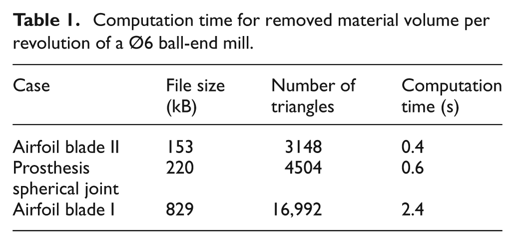
Test parts: (a) airfoil blade I, (b) airfoil blade II and (c) femur prosthesis hemispherical head.
Force model creation
Experimental measurements
The data necessary to train the ANN are obtained from experiments. Orthogonal arrays were preferred to full-factorial experiment for reasons of cost. 29 The purpose of the experiments was to determine the relationship between feed, speed and removed volume per revolution and cutting force along the three main axes for a particular workpiece material.
In this case, the material was aluminium alloy series 2000. The experimental setup consisted of a vertical machining centre (HAAS minimill), a two-fluted ball-end mill of 6 mm diameter made of standard HSS Co8 (type H2535060). Cutting force was measured using a custom-designed and built precision dynamometer consisting of two rigid platens with five spacers between them, the central one being a Kistler piezoelectric three-component sensor type 9602A3201. The sensor has an integral amplifier and was powered by a stabilised regulated power at 20 V and 20 mA. The dynamometer was connected through an intermediate board (NI CB-68LP) to a data acquisition card (NI PCI-6229) supporting up to 250 ksample/s. Magnetically shielded cables were employed. The card was interfaced to the LabVIEW™ program running on a standard personal computer (PC). Sampling rate was set to 1 ksample/s. The dynamometer was duly calibrated using standard precision weights. Figure 4 presents the main parts of the experimental setup.
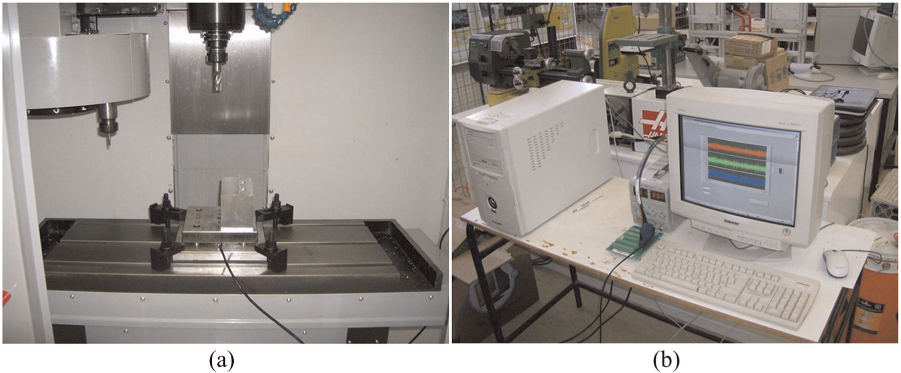
Experimental setup: (a) machine part and (b) computer part.
The material block was bolted onto the upper platen of the dynamometer, and its leftmost planar wall coincided with the vertical plane of symmetry of the dynamometer, passing in fact through the centre of the sensor. A number of straight line passes was planned and executed along the edge of the block each pass materialising one experiment. The area and subsequently the volume of removed material per revolution is calculated according to two variables representing the vertical (da) and horizontal (dr) offset of the edge of the tool from the edge of the workpiece (see Figure 5). There are two cases regarding the relative position of the tool axis and the material edge and two corresponding equations for area calculation
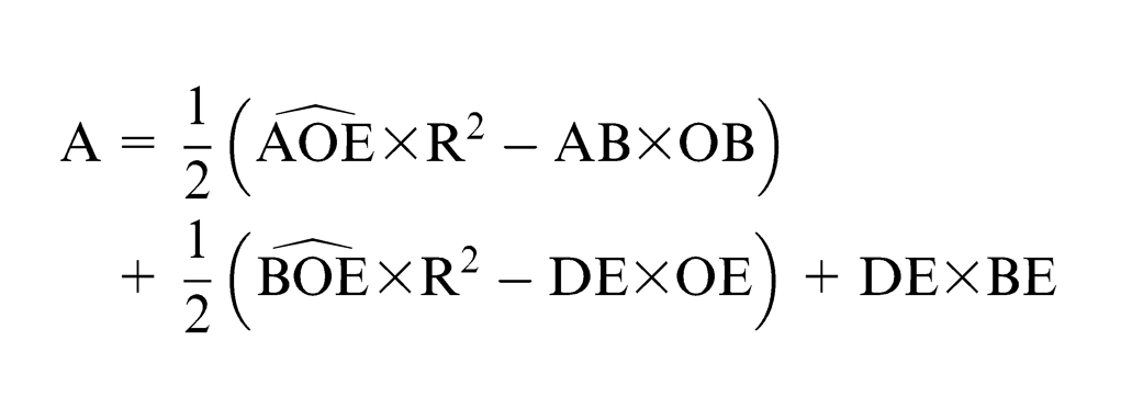
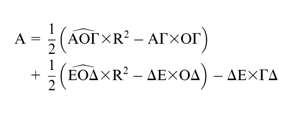
where angles are expressed in radians. The volume of removed material per revolution VR is calculated as

where f denotes feed (mm/min) and n tool angular velocity (r/min).
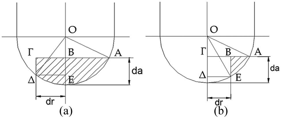
Offset variables between tool and workpiece edge: (a) case I and (b) case II.
In reality, instantaneous material volume removed may be a continuous function of time and so is chip load. However, as an average over a revolution, the material volume removed is constant over the full tool path, due to the constant geometry of the stock and the linear form of the tool path; note also that the number of simultaneously cutting teeth in this particular case is equal to 1. For these reasons, an analytical method is employed to calculate material volume removed. Otherwise, the Boolean calculation which is used in the general methodology would have been employed in this case, too.
Four following levels were selected for each variable:
Feed: 200, 250, 300 and 350 mm/min.
Speed: 2500, 3000, 3500 and 4000 r/min. Speed and feed values were selected according to tool manufacturer instructions and machine tool capabilities.
Vertical offset: 0.25, 0.50, 0.75 and 1 mm.
Horizontal offset: −1, −0.35, 0.35 and 1 mm, negative values corresponding to tool offset towards the inside of the workpiece and positive values towards the outside.
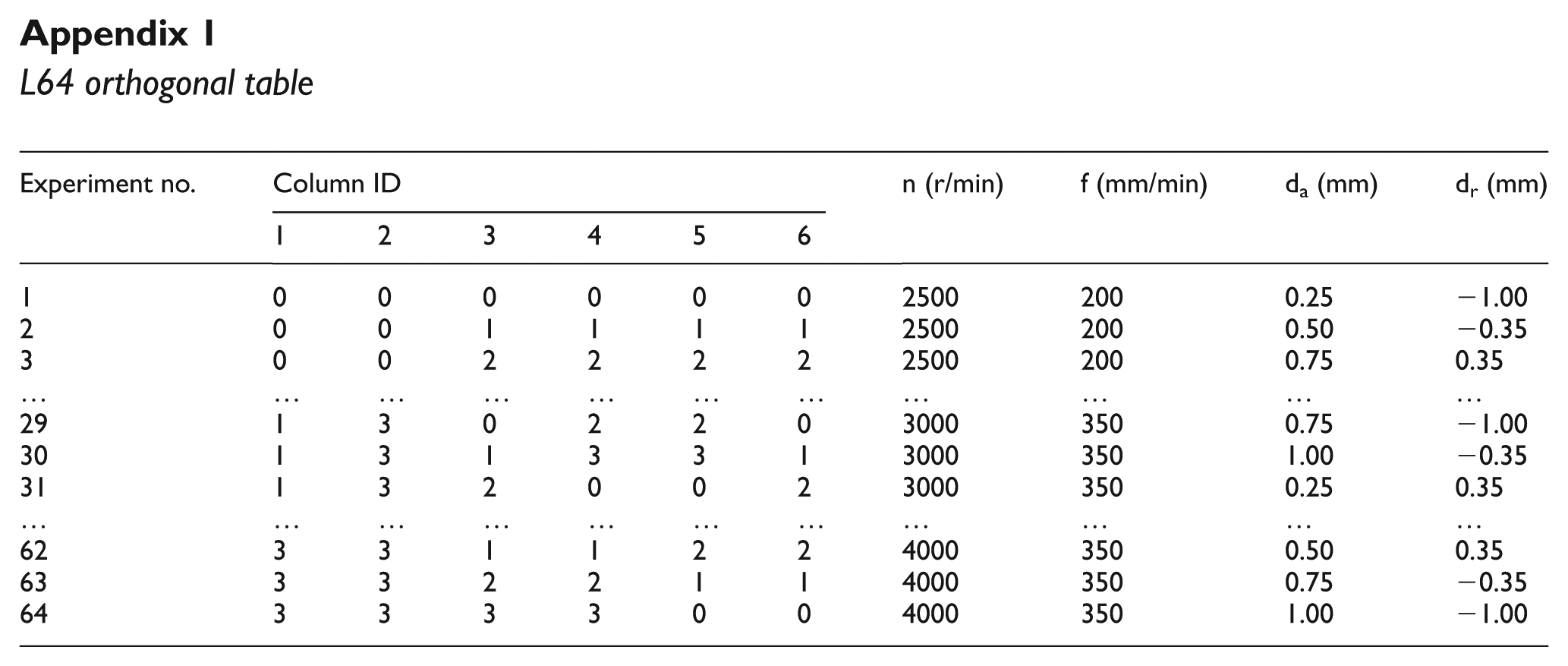
The most suitable orthogonal table was modified L64 because it can accommodate six main parameters with four levels each. 29 A full-factorial experiment would need 44 = 256 cutting passes, whereas L64 needs just 64, that is, 4 times less.
The most probable interaction is between rotational speed and feed and is accommodated in column 3 of the table. Rotational speed was accommodated in column 1, feed in column 2, vertical offset in column 4 and horizontal offset in column 6. Substituting the parameter levels and deleting the columns that did not contain any parameters yields the final DoE table (see Appendix 1).
Cutting force signal was recorded for the full duration of cut. Measurement of the maximum force was based on a 10-revolution sample (see Figure 6). Average maximum force over the 10 samples of each experiment was retained, and the corresponding results are shown in Table 2, where horizontal/vertical offsets are replaced by the respective material removal volume per revolution.
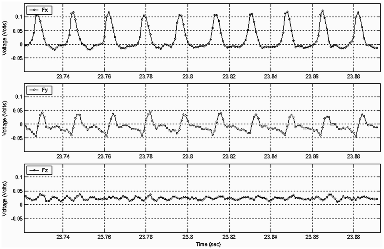
Cutting force signal sample.
Experimental results.
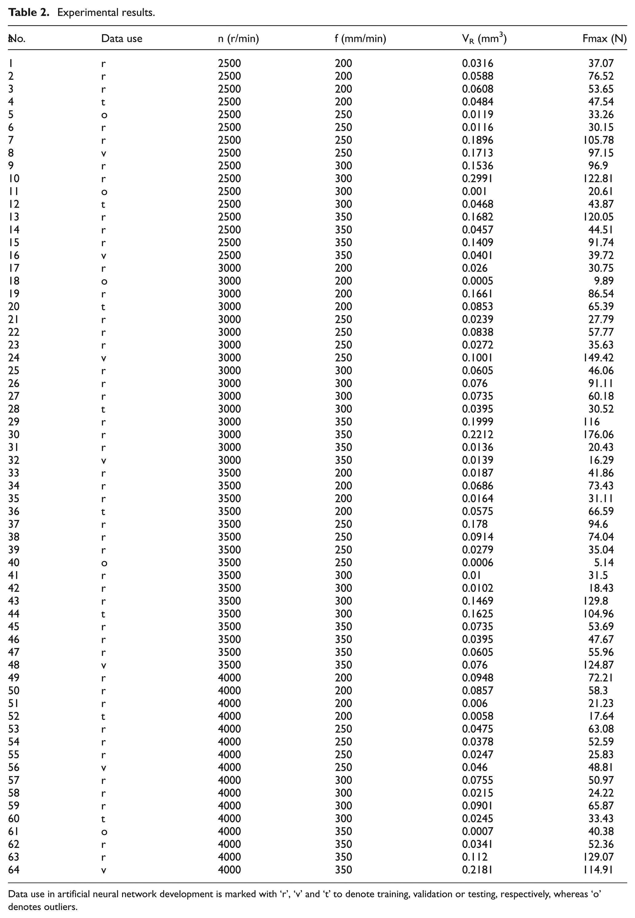
Data use in artificial neural network development is marked with ‘r’, ‘v’ and ‘t’ to denote training, validation or testing, respectively, whereas ‘o’ denotes outliers.
ANN development
An ANN is a simple computational model of human brain functioning consisting of a large number of neurons interconnected using weighting. A neuron can have many inputs but only one output which in turn is the input of other neurons. The output of any neuron is computed as the weighted sum of its inputs becoming an argument of the so-called activation function. The process of finding the values of weights is called training and needs an adequate number of examples constituting the training set. Feedforward–feedback propagation ANNs use popular training algorithms based on the so-called delta rule, which calculates a corrective increment of the weight values in iterative steps (epochs). An ANN response to unknown input is characterised as generalisation performance and employs the testing set of examples. The validation subset is used to ensure that when the error remains constant for a predefined number of epochs or starts to increase rapidly, training should stop to avoid overfitting. 30
The most important problem in developing a feedforward ANN model is that there is no prior guarantee that the model will perform well for the problem at hand because the ANN architecture is usually determined by trial and error based on intuition and experience. The ANN for force prediction that was necessary in this work was developed according to a proprietary automated methodology and associated software tool analytically presented elsewhere, 31 and its main features being summarised next.
Software tool used
The software tool used determines the number of hidden layers and the number of neurons in each of them. The solution space consists of all the different combinations of hidden layers and hidden neurons, that is, of all ANN architectures, and a GA searches it for the optimum combination according to predefined criteria.
GAs breed coded solution populations using biological operators essentially imitating species improvement though reproductive generations. The essential parts of a GA 32 are (1) a genetic representation of possible solutions to the problem (problem coding), (2) an objective function used in evaluating possible solutions in terms of their fitness to survive in the ‘environment’ specific to the problem at hand, (3) genetic operators that diversify the genetic material of descendants compared to that of the ancestors and (4) a way to create an initial population of solutions.
In this work, an indirect encoding scheme was selected, that is, only information about the number of hidden layers and number of hidden neurons in each layer contained in the chromosomes. The problem’s parameters are coded in a 10-bit binary chromosome. The first and second group of 5 bits correspond to the number of neurons in the first and second hidden layers, respectively, that is, 31 maximum in each. Four criteria are combined in the evaluation function employed.
Training error Et, as the first criterion, is the average of the absolute values of relative error. The second criterion is the ANN generalisation error Eg, assessed as the average of the absolute values of relative error, too.
The third criterion is the feedforward architecture criterion (FFAC), which favours smaller architectures, by applying a penalty term to the objective function, in order to avoid overfitting the training data, by decreasing complexity of the ANN. In general FFAC = αef(x), where α is a constant and f(x) is a function of the total number of weights and biases of the ANN. The fourth criterion concerns solution space consistency (SSCC). This computes the generalisation error for each case of the testing subset separately and applies a penalty when outlier cases, showing a very high generalisation error, are identified. Characterisation of generalisation error is, of course, mostly case dependent or even user biased. Thus, the objective function is formulated as FFAC × SSCC × (Et+ Eg).
The corresponding software was developed as a tool in MATLAB to be efficiently used with little to no experience in the fields of ANNs and GAs, while maintaining the generality of the methodology. When the application terminates, the best ANN architecture is directly accessed from the MATLAB workspace.
Result
Data in Table 1 were split into training, validation and testing subsets consisting of 44, 7 and 8 vectors (68.75%, 11% and 12.5%, respectively). Five vectors were treated as outliers, that is, it was considered that they could influence ANN training in a negative way and were thus removed.
In the GA, the population size was 25, maximum number of generations was set to 50, and 23 new offspring were generated per generation. Genetic operators were not changed from default. Selection is performed through uniform stochastic sampling, new offspring are produced through single-point crossover and mutation probability is set at 5%.
The input layer had three neurons and the output layer just one. Furthermore, activation function at all but the input layer was hyperbolic tangent, whereas at the input layer, it was the identity function. The FFAC criterion is expressed as
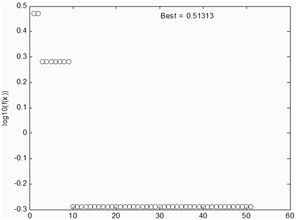
Evolution of the GA evaluation function with the number of generations.
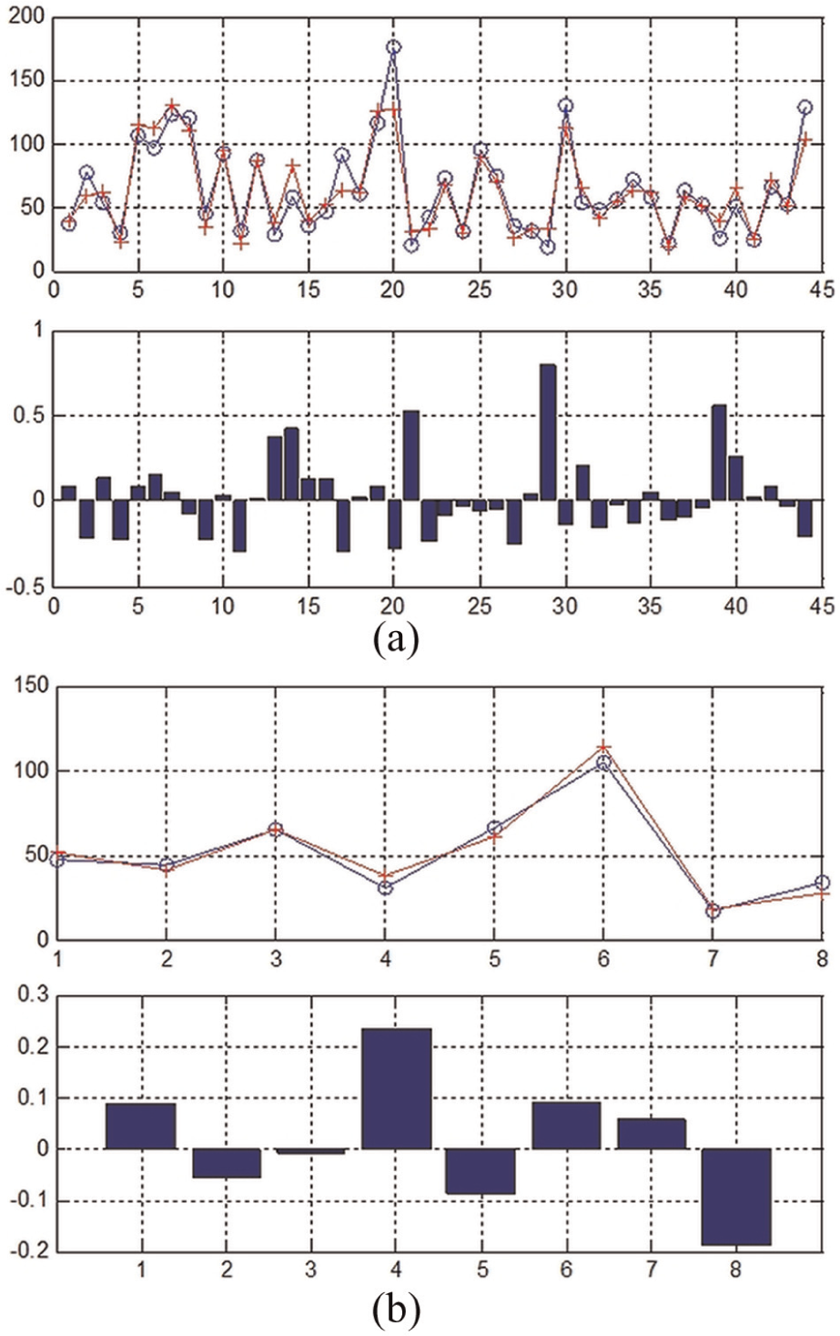
(a) Target values (circles) and ANN response (crosses) for training (left) and testing (right) subsets and (b) relative error for training (left) and testing (right) subsets.
Input parameter values are readily available for any point along the tool path, that is, feed and speed through the G-code, removed volume per revolution through the method developed. Cutting force is output by the ANN.
Feed and speed optimisation
Optimisation is implemented through a GA which makes use of the ANN model as a cutting force prediction method in its evaluation function. This approach was selected for two reasons: first because there are multiple combinations of feed and speed that may result in the same force, and second, although increasing spindle speed with or without simultaneously reducing feed is qualitatively known to lead to lower forces and vice versa, this cannot be computed quantitatively in the general case.
It should be noted from the start that optimisation procedure refers to discrete points on the tool path. Each point is input to the GA by an identification number representing its order in the series of discrete points of the tool path. The same procedure needs to be repeated for as many points as required along the tool path.
In order to identify the parts of each tool path where optimisation is necessary, it is necessary to construct a diagram of force variation across all points of interest on the tool path. The parts where force patterns are different to what is desired can be identified by inspection or even by custom software. Visual inspection suffices for the purposes of this work. Force calculation is straightforward by computing the material volume removed per tool revolution and then feeding the ANN with this information together with the designated feed and speed for the particular point under consideration. The solid model of the part, be it in its initial condition or in its as-roughed condition (depending on whether the tool path refers to roughing or finishing, respectively), must be available so as to enable computation of the material volume removed.
The GA is in fact quite simple, and for this reason, the reader is referred to standard textbooks outlining the basics of GAs. 32 It was implemented in MATLAB making use of the dedicated GA function library. Chromosome encoding consists of two binary strings, namely, one for feed and one for speed. GA setup process starts by setting the upper and lower limits of speed and feed values. This takes into account the respective ranges specified by the cutting tool manufacturer as well as the capabilities of the machine tool, for example, regarding maximum spindle speed, maximum power available and so on. Next, population size (= 10), maximum number of generations (= 100) and percentage of population of offspring to be created in each generation are specified (= 80%).
Genetic operators used are the classic ones, that is, selection, crossover and mutation. Selection operator is of the stochastic uniform type. Crossover is of the single-point type with constant probability of recombination (= 70%). Standard probabilistic mutation is applied with low probability (= 5%). If any of the chromosomes contain values that are outside these limits, a large number (penalty) is imposed as the result of the evaluation function thereby avoiding evaluation of the respective chromosome.
The evaluation function can have different forms. In the simplest case, it is the difference between the computed and the desired force values. Minimisation of this difference is sought since it also leads to decrease in force variations. The desired force value may be determined according to different strategies. One strategy involves calculating the mean force separately for each section of the tool path, where intense variation of force exists. This mean force value can be applied as the desired force value across all points in the tool path under consideration. Another strategy involves setting as desired force value for the nth point on the tool path the actual force of the previous point, after optimisation of the latter, that is, in an iterative way. Most importantly, any force pattern may be set as desirable by suitably defining the evaluation function.
Results and discussion
The method presented above has been tried in a variety of sculptured surface finishing cases, concerning different geometry and machining strategies, some of them being depicted in Table 1. Tool path derivation and simulation of material removal was carried out on SolidCAM™. A sample case is presented next.
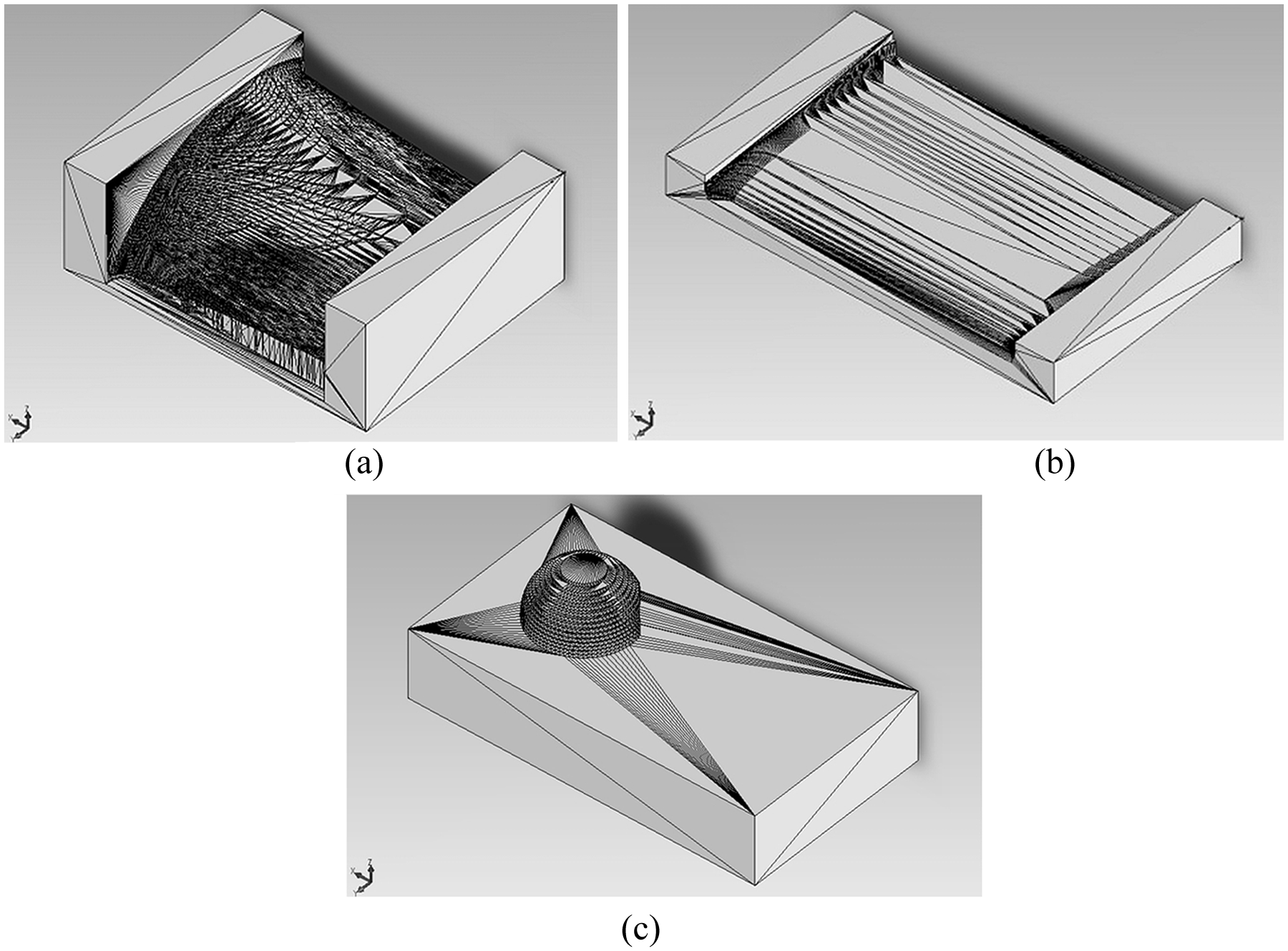
The part was first roughed using a hatching strategy on successive parallel XY planes at a distance of 1 mm from each other, using a 20-mm end mill. Pass overlap on each plane was selected at 50% of tool diameter. The characteristic staircase effect on the roughed surface constituted the baseline for finish machining with a 6-mm ball-end tool and circular offset pattern at successive XY planes at a variable distance from each other so as to achieve a maximum scallop height of 10 µm (see Figure 9). Feed was selected at 200 mm/min and spindle speed at 3000 r/min, according to tool manufacturer recommendation. Interpolation distance along the tool path was 16 µm, while material removal volume was calculated for 10-mm path sections.
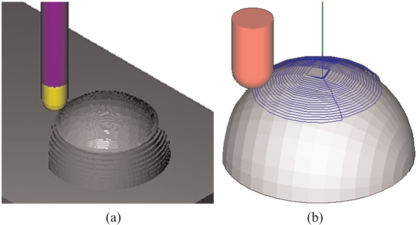
Hemisphere finish machining: (a) simulation half-way through and (b) tool path pattern.
A total of 10 sections have been identified by observing force variation before optimisation (see Figure 10(a)). For each of these sections, the average force is calculated, and for all points exhibiting a difference larger than 10% from this value, the optimisation procedure is executed in order to minimise this difference. The optimised commanded feed and speed patterns as well as the resulting force pattern for the full tool path are given in Figure 10. A statistical overview per tool path section is given in Table 3.
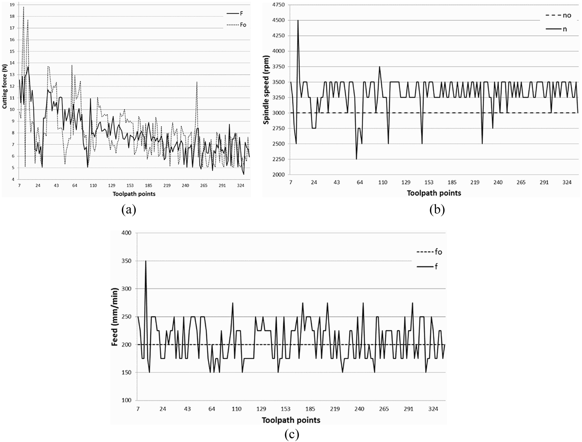
Optimisation results: (a) cutting force (F0 before optimisation/F after optimisation), (b) spindle speed (n0 = constant before optimisation/n after optimisation) and (c) feed (f0 = constant before optimisation/f after optimisation).
Statistical presentation of optimisation results.
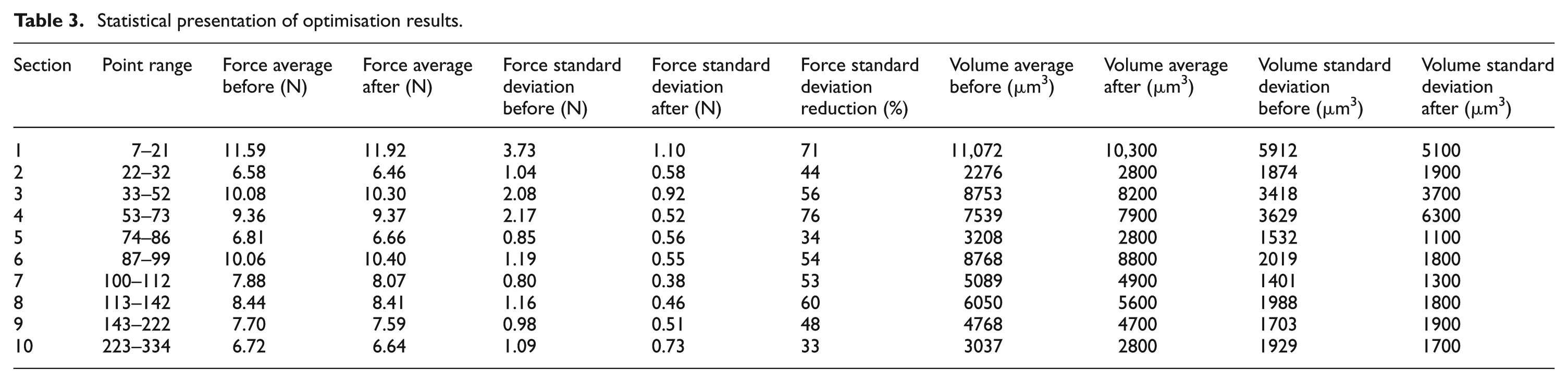
It becomes fairly obvious that reduction of force standard deviation after optimisation is significant, in the range of 33%–71%, while mean force does not vary much compared to its initial value, exactly as intended. By contrast, volume mean differs more significantly before and after optimisation and its standard deviation may well increase significantly after optimisation in an effort to drive forces at the individual points of each section as close to the average value as possible.
According to the results presented, cutting force can be increased or reduced as necessary, in an expected way, that is, force reduction is achieved by lowering feed and/or increasing spindle speed and vice versa.
Optimised cutting force is increased in most cases, thus indirectly verifying the estimate that cutting tool manufacturers suggest conservative cutting conditions. This is achieved through considerable increase of feed (per minute) hence decrease of machining time. Material volume removed per revolution is approximately constant for each circular pass, and the optimisation process tends to yield similar cutting condition pairs, showing consistency. The major advantage, though, is decrease of dimensional accuracy and surface quality problems due to low variation in cutting force.
The reader is reminded that even if the influence of further factors on cutting force (e.g. machine tool and cutting tool wear) cannot be explicitly modelled, construction of the ANN through experimental data takes these factors into account implicitly. Before optimisation, where both feed and spindle speed remain constant, force value variation predicted by the ANN should follow the relevant variation of material volume removed, which depends on part geometry and tool path applied.
It is important to note the paramount importance of the ANN cutting force model in the overall methodology. This is employed first for calculating the force variation along the tool path in order to locate the sections where variation is intense. It is also employed in the optimisation procedure, in the evaluation function of the GA, repeatedly. An inaccurate ANN would have negative effect on both steps of the method, namely, in the first one, false force variation patterns could easily disorientate optimisation effort, leading it to focus on irrelevant parts of the tool path at the same time neglecting important ones; in the second step, it would simply lead to wrong feed and speed values.
Success in ANN modelling is ensured by the systematic methodology and software of Benardos and Vosniakos 31 and not just as a result of experience, intuition or even luck. No experience is required by the user neither in the field of ANNs nor in GAs. The necessary time for executing the software implemented methodology (in the order of several minutes in the case study presented) is much less compared to the trial-and-error common practice (in the order of several days).
Note that the approach’s success is due among other things to the fact that (1) this deals with the noise stemming from a phenotype’s fitness representing the genotype’s fitness, (2) early stopping is used resulting in less computation time and better performing ANNs and (3) the generalisation error is not simply evaluated, but it is directly calculated during the evolutionary process by using the testing subset after each architecture is trained.
The necessary time to perform optimisation at one point on the tool path mainly depends on the size of the file describing the initial form of the part. Larger computational time is due to the routine for calculating volume of material removed, see section ‘Volume of material removed per revolution’, within the cutting force evaluation process, and is of the order of seconds on a Core i5 processor at 3.2 GHz with 8 GB RAM. The total time required is also connected to the population size of the GA and the maximum number of generations, that is, the total number of evaluations to be performed. This was in the order of 1 h.
Regarding implementation, the multitude of software platforms used (MATLAB, Visual Basic and SolidWorks) was adopted so as to avoid programming from scratch what is already available in each of these platforms, which is usual practice in prototyping applications.
Conclusion and further work
Feed and speed in sculptured surface machining were optimised by a GA that makes use of a ANN model of the cutting force, so as to ensure reduction in variation of cutting force at selected regions along the tool path. The main contributions of this work are that
Both feed and speed are optimised at the same time;
The cutting force pattern can be defined at will and combined with other criteria and constraints;
The cutting force model is based on simple measurements that capture the characteristics of the particular equipment employed.
The method is readily applicable in high-speed milling where, due to high inertial forces and small tool diameters, if employed, cutting force variations are much more interesting and potentially crucial since they can lead to premature wear, vibration or even breakage of the tool, hence minimisation or control of these variations within desirable patterns become even more important.
Central to the methodology is calculation of the volume removed per spindle revolution by making use of solid modelling operators of existing CAD/CAM software, as well as the solid model representation of the initial workpiece shape. However, this calculation may be time-consuming depending on the CAD system architecture and routines being evoked. Therefore, although it is possible to determine volume removed at any point of the tool path, in order to reduce computation time, the tool path may be discretised with varying density as the user desires.
In reality, instantaneous material volume removed may be a continuous function of time and so may the chip load be; however, such a calculation is not realistically possible for long tool paths and some sort of averaging out is necessary. The simplification involved refers to the relatively low number of angular and corresponding very small feed displacements during one full tool revolution. The number of teeth is taken into account as part of the tool solid model, whereas the angle of engagement for each tooth comes directly into play in the relevant Boolean intersection with the part’s solid model.
In this work, the ANN model of the cutting force has an optimum architecture that is determined in a rigorous way as opposed to trial-and-error approaches often followed. It takes into account both control parameters of the machining process, that is, feed and spindle speed, as well as part geometry through material volume removed per spindle revolution. Moreover, the properties of the equipment are also taken into account since the model is based on experimental data obtained from the very equipment used. This is an important advantage of this approach.
The use of an ANN to model the cutting force and the possibility to handle each point of the tool path separately in the GA allows for different strategies of optimisation as desired. Practically, this is equivalent to the possibility of defining desired cutting force variation patterns for selected areas of the part.
Optimisation of rough machining is perfectly possible, too, although this has not been demonstrated. This should follow exactly the same method, provided that cutting force constitutes the main criterion. For example, instead of reduction of variation in cutting force, its maximisation could be pursued up to a certain upper limit connected with machine dynamics, power availability, cutting tool strength and so on. A direct extension of this work may also involve constraints, such as maximum feed variation allowed and additional evaluation criteria, for example, machining time. In addition, desirable force patterns may be defined for specific machined features so as to achieve a kind of standardisation in optimisation criteria. In addition, the use a solid modelling engine rather than a complete CAD system would most probably make calculation of machined volume per revolution much faster. Finally, note that extension towards four- or five-axis machining is only a matter of adding the appropriate interpolation routines to calculate tool pose at the points of interest along the tool path.
Footnotes
Appendix
L64 orthogonal table
| Experiment no. | Column ID |
n (r/min) | f (mm/min) | da (mm) | dr (mm) | |||||
|---|---|---|---|---|---|---|---|---|---|---|
| 1 | 2 | 3 | 4 | 5 | 6 | |||||
| 1 | 0 | 0 | 0 | 0 | 0 | 0 | 2500 | 200 | 0.25 | −1.00 |
| 2 | 0 | 0 | 1 | 1 | 1 | 1 | 2500 | 200 | 0.50 | −0.35 |
| 3 | 0 | 0 | 2 | 2 | 2 | 2 | 2500 | 200 | 0.75 | 0.35 |
| … | … | … | … | … | … | … | … | … | … | … |
| 29 | 1 | 3 | 0 | 2 | 2 | 0 | 3000 | 350 | 0.75 | −1.00 |
| 30 | 1 | 3 | 1 | 3 | 3 | 1 | 3000 | 350 | 1.00 | −0.35 |
| 31 | 1 | 3 | 2 | 0 | 0 | 2 | 3000 | 350 | 0.25 | 0.35 |
| … | … | … | … | … | … | … | … | … | … | … |
| 62 | 3 | 3 | 1 | 1 | 2 | 2 | 4000 | 350 | 0.50 | 0.35 |
| 63 | 3 | 3 | 2 | 2 | 1 | 1 | 4000 | 350 | 0.75 | −0.35 |
| 64 | 3 | 3 | 3 | 3 | 0 | 0 | 4000 | 350 | 1.00 | −1.00 |
Declaration of conflicting interests
The authors declare that there is no conflict of interest.
Funding
This work was funded as project number 01EΔ131 of the PENED2001 action at 75% by the European Union – European Social Fund and 25% the Greek State – Ministry of Development, General Secretariat for Research and Technology and the Private Sector (companies Axon Engineering S.A. and VIORAL S.A.) under Measure 8.3 of the Operational Programme ‘Competitiveness’ 2000–2006 of the Third Community Support Programme.