Sage Journals: Discover world-class research

Abstract

In the field of large-scale dimensional metrology, new distributed systems based on different technologies have blossomed over the last decade. They generally include (1) some targets to be localized and (2) a network of portable devices, distributed around the object to be measured, which is often bulky and difficult to handle. The objective of this article is to present some diagnostic tests for those distributed large-scale dimensional metrology systems that perform the target localization by triangulation. Three tests are presented: two global tests to detect the presence of potential anomalies in the system during measurements and one local test aimed at isolating any faulty network device(s). This kind of diagnostics is based on the cooperation of different network devices that merge their local observations, not only for target localization but also for detecting potential measurement anomalies. Tests can be implemented in real time, without interrupting or slowing down the measurement process. After a detailed description of the tests, some practical applications on Mobile Spatial coordinate Measuring System-II (MScMS-II) – a distributed large-scale dimensional metrology system based on infrared photogrammetric technology, recently developed at DIGEP-Politecnico di Torino – are presented.

Keywords

Large-scale dimensional metrology distributed measuring system triangulation model-based redundancy cooperative diagnostics online diagnostics statistical test

Introduction and literature review

In the last decade, there has been an increasing development of distributed dimensional metrology systems, that is, instruments consisting of multiple devices that are positioned around the object to be measured and cooperate during the measurement activity.^1–3 The majority of these systems have been developed in the field of large-scale dimensional metrology (LSDM), concerning the measurement of medium- to large-sized objects (i.e. according to the definition by Puttock,⁴ ‘objects with linear dimensions ranging from tens to hundreds of meters’), in industrial environments. Typical industrial applications are (1) reconstruction of curves/surfaces for dimensional verification and (2) assembly of large-sized mechanical components, in which levels of accuracy of several tenths of millimetres are generally tolerated.

The reason behind the development of distributed LSDM systems is simple: arranging a portable measuring instrument around the object to be measured is often more practical than the vice versa.⁵

Existing measuring systems differ in technology (e.g. laser optical, photogrammetric, interferometric and ultrasound); some of these are consolidated and available on the market, while others are only prototypes. Table 1 classifies some systems, reporting key features and bibliographic references for the reader.

Table 1.

Classification of some of the existing distributed LSDM systems.

Name	Technology	Current level of development	Localization technique	Bibliographic reference
Nikon iGPS	Laser optical	Commercial	Triangulation	Maisano et al.⁶
3rd Tech HiBall	Infrared, LED	Semi-commercial	Triangulation	Welch et al.⁷
Multiple Laser Trackers	Interferometric, ADM	Commercial	Multilateration	NPL⁸
MScMS-I	Ultrasound	Prototype	Multilateration	Franceschini et al.¹
MScMS-II	Infrared photogrammetric	Prototype	Triangulation	Galetto et al.⁹

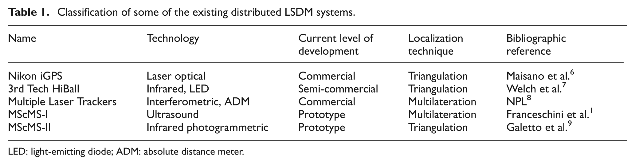
LED: light-emitting diode; ADM: absolute distance meter

The common features of these systems are as follows (see Figure 1):

A network of devices distributed around the object to be measured;

A hand-held probe for measuring the spatial Cartesian coordinates (XYZ) of the points of interest;

A centralized data processing unit (DPU), which receives local measurement data from network devices.

Figure 1.

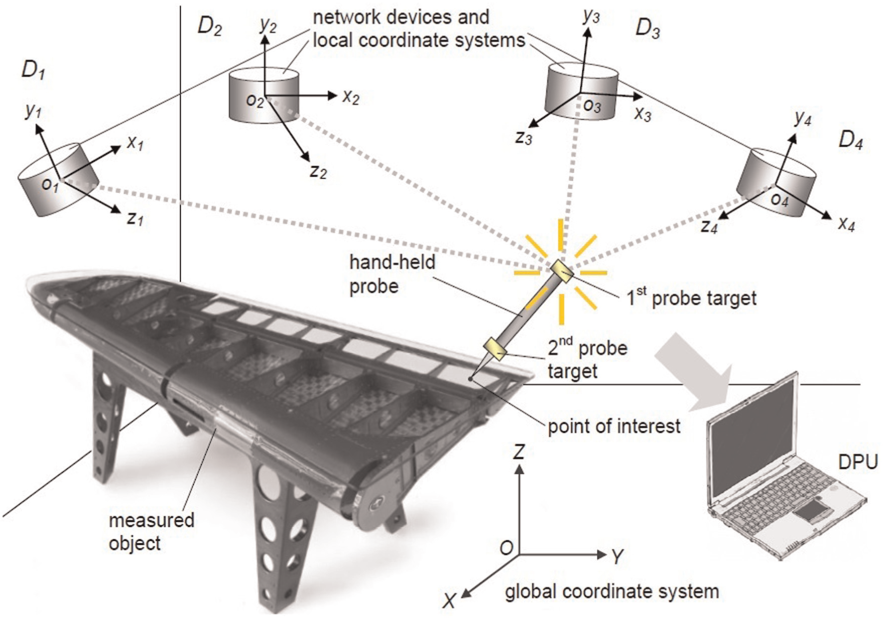
Schematic representation of a generic distributed LSDM system.

The probe is equipped with some targets and a stylus, which is in contact with the point of interest. A probe calibration process allows to know the relative positions between probe targets and stylus. The localization of probe targets allows to determine the probe position/orientation and – consequently – the stylus position. Since it acts as a filter, the stylus radius is chosen depending on the measurement task. This is a typical problem of classical contact coordinate measuring machines (CMMs); for more information, see Butler.¹⁰

In certain cases (e.g. for Mobile Spatial coordinate Measuring System-II (MScMS-II)), probe targets are passive sensors, while in others (e.g. for iGPS), they are active and can have a processing capability which makes them able to perform local measurements (typically angles or distances) with respect to network devices.

As shown in Table 1, there are two typical techniques for localizing probe targets:¹⁰

Triangulation, using the angles subtended by the targets, from the local perspective of at least two network devices;

Multilateration, using the distances between the targets and at least three network devices.

The number of devices involved in the localization of a target depends on their mutual positioning/orientation and communication range. For distributed LSDM systems, as well as for metrological systems in general, reliability of measurements is essential and can be increased by the use of real-time diagnostic tools able to detect measurement accidents and discard/correct (part of) the measurement results.

The purpose of this article is to present some novel statistical tests for the online diagnostics of distributed LSDM systems based on triangulation, in the case of quasi-static measurements – that is, targets are stationary or are moved at very low speeds during their localization. These tests make it possible to identify possible measurement accidents and, subsequently, to isolate the (potentially) faulty network devices. This kind of diagnostics can be classified as cooperative since it is based on the cooperation of different network devices that merge their local angular measurements.

The three statistical tests that will be discussed are divided in two categories:

Two global tests aimed at evaluating the reliability of measurements, based on their variability.

A local test that – when a measurement is not considered reliable by (at least one of) the global tests – identifies the potentially faulty device(s) and (temporarily) excludes them from the measurement process, without interrupting it.

After a detailed description of each test, some real application examples using MScMS-II – that is, a prototypical distributed LSDM system based on infrared photogrammetric technology, recently developed at the Industrial Metrology and Quality Engineering Laboratory of DIGEP-Politecnico di Torino – are shown.

The remaining of this article is structured in four sections. Section ‘Background information’ provides some background information, which is helpful to grasp the subsequent description of statistical tests: (1) basic concepts concerning distributed LSDM systems’ diagnostics, (2) a general description of the localization problem for systems based on triangulation and (3) a brief description of MScMS-II, on which the diagnostic tests will be implemented. Section ‘Online diagnostic tests’ provides a detailed description of the statistical tests (global and local, respectively) with some experimental examples. Finally, Section ‘Implications, limitations and future research’ summarizes the original contributions of this research, focusing on its implications, limitations and possible future developments.

Background information

Basic concepts concerning diagnostics

In general, the concept of reliability of a measurement is defined as follows: For each measurable quantity x, it can be defined an acceptance interval [LAL, UAL] (where LAL stands for lower acceptance limit and UAL for upper acceptance limit).¹ The measure x_M of the quantity x, produced by a measurement system, is considered reliable if $x_{M} \in [L A L, U A L]$ .

Type I and Type II probability errors (misclassification rates), respectively, correspond to

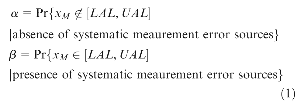
\begin{array}{l} α = Pr {x_{M} \notin [L A L, U A L] | absence of systematic meaurement error sources} \\ β = Pr {x_{M} \in [L A L, U A L] | presence of systematic meaurement error sources} \end{array}

(1)

Usually, LAL and UAL are defined considering the natural variability of the measurement system (which is linked to its metrological characteristics of accuracy, reproducibility, repeatability, etc.), in the absence of systematic error sources.¹¹ The authors are aware that systematic errors can never be eradicated completely, especially when they are relatively small and interrelated with each other. The assumption of only random errors is not valid in general, even though could be adequate for many applicative situations.

For distributed systems, local anomalies of one or more network devices can distort or even compromise the whole measurement. On the contrary, when these anomalies are recognized, the measurement results can be corrected, (temporarily) excluding malfunctioning device(s). This is the reason why distributed systems are – to some extent – rather ‘vulnerable’ but can be successfully protected by appropriate diagnostic tools.

For distributed systems, a typical diagnostic approach is based on the so-called model-based redundancy, where the replication of a physical instrumentation – which is typical of the physical redundancy approach – is substituted by the use of appropriate mathematical models.¹² These models may derive from physical laws applied to experimental data or from self-learning method (e.g. neural networks) and allow the detection of system failures by comparing measured and model-elaborated process variables. This diagnostic approach is made possible by the fact that for distributed systems, the number of network devices generally involved in a measurement is greater than the number strictly necessary for performing the localization of target(s).

This type of diagnostics is based on the cooperation of network devices, whose local observations are used in conjunction, not only for target localization but also for detecting possible measurement anomalies or accidents.

Diagnostic tools based on this philosophy are implemented for GPS-assisted aircraft navigation, where the global positioning system (GPS) can be seen as a very large-scale-dimensional metrology distributed system, in which localization is performed by multilateration.¹³ Furthermore, Franceschini et al.¹⁴ give a detailed description of some online diagnostic tools for MScMS-I, an indoor distributed LSDM system based on multilateration.

As mentioned in Section ‘Introduction and literature review’, this diagnostic generally includes two types of tests (global and local), aimed, respectively, at (1) evaluating unreliable measurements and (2) identifying and (temporarily) excluding purportedly faulty network devices. The flowchart in Figure 2 illustrates a typical sequence of implementation of these tests.

Figure 2.

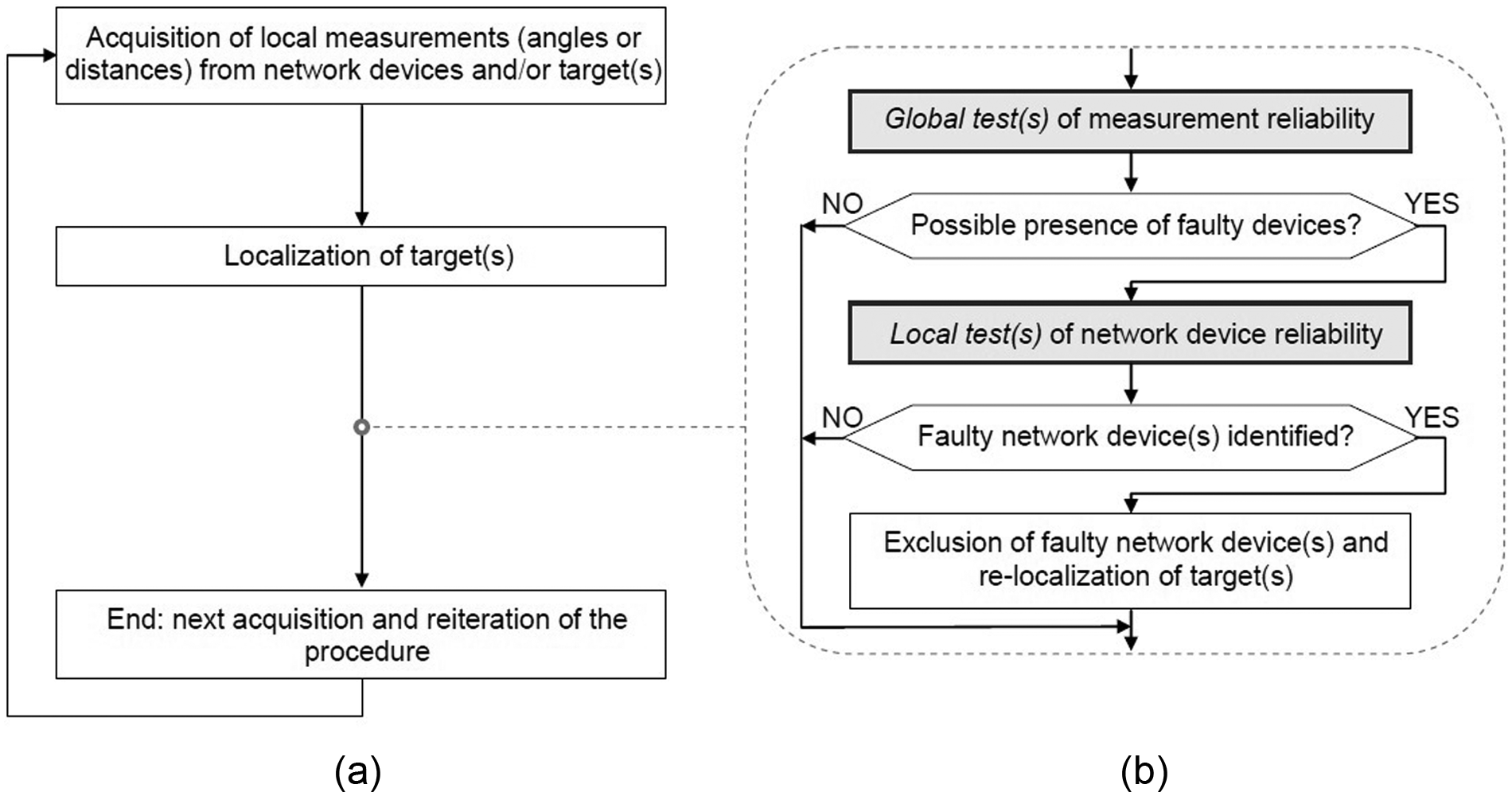
Flowchart showing the logical implementation sequence relating to the online diagnostic tests: (a) localization procedure and (b) online system diagnostics.

The triangulation problem

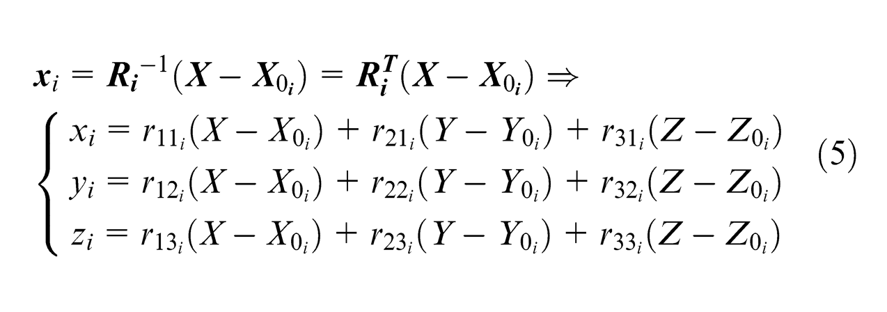
Figure 1 depicts a distributed LSDM system consisting of a number of network devices (D₁, …, D_N) positioned around the object to be measured. OXYZ is a global Cartesian coordinate system. Each of the devices has its own spatial position and orientation; for each ith device, it is defined a local coordinate system o_ix_iy_iz_i, roto-translated with respect to OXYZ.

A general transformation between a local and the global coordinate system is given by

\begin{array}{l} X = R_{i} x_{i} + X_{o i} \Rightarrow [\begin{matrix} X \\ Y \\ Z \end{matrix}] \\ = [\begin{matrix} r_{11_{i}} & r_{12_{i}} & r_{13_{i}} \\ r_{21_{i}} & r_{22_{i}} & r_{23_{i}} \\ r 31_{i} & r_{32_{i}} & r_{33_{i}} \end{matrix}] [\begin{matrix} x_{i} \\ y_{i} \\ z_{i} \end{matrix}] + [\begin{matrix} X_{o_{i}} \\ Y_{o_{i}} \\ Z_{o_{i}} \end{matrix}] \end{array}

(2)

R_i is a rotation matrix, in which elements are functions of three rotation parameters (see Figure 3)

R_{i} = [\begin{matrix} cos ϕ_{i} cos κ_{i} & - cos ϕ_{i} \sin κ_{i} & \sin ϕ_{i} \\ cos ω_{i} \sin κ_{i} + \sin ω_{i} \sin ϕ_{i} cos κ_{i} & cos ω_{i} cos κ_{i} - \sin ω_{i} \sin ϕ_{i} \sin κ_{i} & - \sin ω_{i} cos ϕ_{i} \\ \sin ω_{i} \sin κ_{i} - cos ω_{i} \sin ϕ_{i} cos κ_{i} & \sin ω_{i} cos κ_{i} + cos ω_{i} \sin ϕ_{i} \sin κ_{i} & cos ω_{i} cos ϕ_{i} \end{matrix}]

(3)

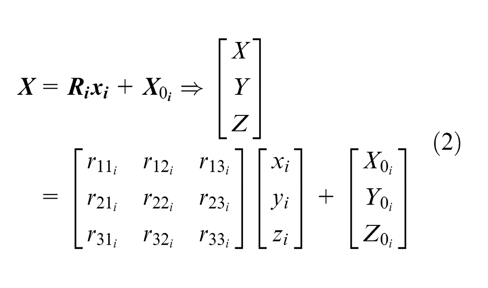
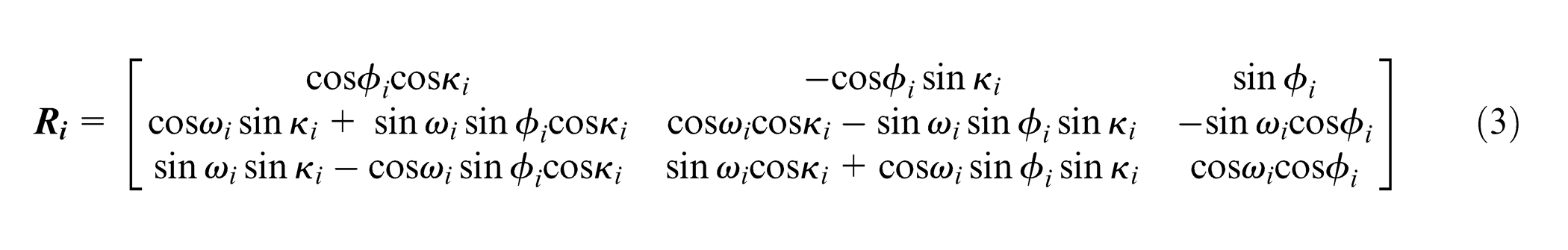
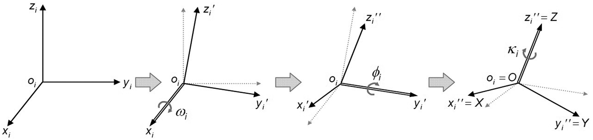
where ω_i represents a counterclockwise rotation around the x_i axis; ϕ_i represents a counterclockwise rotation around the new y_i axis (i.e. ${y'}_{i}$ ), which was rotated by ω_i; κ_i represents a counterclockwise rotation around the new z_i axis (i.e. ${z ″}_{i}$ ), which was rotated by ω_i and then ϕ_i.

Figure 3.

Rotation parameters regarding the transformation between a local coordinate system (o_ix_iy_iz_i) and the global one (OXYZ).

$X_{0 i} = {[X_{0_{i}}, Y_{0_{i}}, Z_{0_{i}}]}^{T}$ are the coordinates of the origin of o_ix_iy_iz_i, in the global coordinate system OXYZ. The angle convention introduced before is quite common for this kind of geometrical problem.

The (six) location/orientation parameters related to each network device (i.e. $X_{0_{i}}, Y_{0_{i}}, Z_{0_{i}}$ , ω_i, ϕ_i, κ_i) are treated as known parameters, since they are measured in an initial calibration process. This process may vary depending on the specific technology of the measuring system; however, it generally includes multiple measurements of some calibrated artefacts within the measurement volume and is characterized by a high level of automation that makes the whole operation relatively fast and efficient.¹⁵

The point to be located is P ≡ (X, Y, Z). From the local perspective of each ith device, two angles – that is, $θ_{c_{i}}$ (azimuth) and $ϕ_{c_{i}}$ (elevation) – are subtended by the line passing through P and a local observation point, which is assumed as coincident with the origin o_i≡ (0, 0, 0) of the local coordinate system (see Figure 4). Precisely, $ϕ_{c_{i}}$ describes the inclination of segment o_iP with respect to the plane x_iy_i (with a positive sign when z_i>0), while $θ_{c_{i}}$ describes the counterclockwise rotation of the projection (o_iP′) of o_iP on the x_iy_i plane, with respect to the x_i axis. For each ith local coordinate system, the two angles are given, respectively, by

\begin{matrix} θ_{c_{i}} = {tan}^{- 1} \frac{y_{i}}{x_{i}} & {\begin{cases} if x_{i} \geq 0 then - \frac{π}{2} \leq θ_{c_{i}} \leq \frac{π}{2} \\ if x_{i} < 0 then \frac{π}{2} < θ_{c_{i}} < \frac{3 π}{2} \end{cases} \\ ϕ_{c_{i}} = {tan}^{- 1} \frac{z_{i}}{\sqrt{{x_{i}}^{2} + {y_{i}}^{2}}} & {- \frac{π}{2} \leq ϕ_{c_{i}} \leq \frac{π}{2} \end{matrix}

(4)

Figure 4.

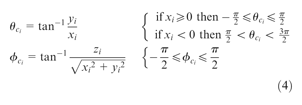
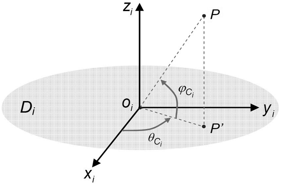
For a generic network device (D_i), two angles – that is, $θ_{c_{i}}$ (azimuth) and $ϕ_{c_{i}}$ (elevation) – are subtended by a line joining the point P (to be localized) and the origin o_i of the local coordinate system o_ix_iy_iz_i.

Regarding the two angles in equation (4), the subscript ‘c_i’ means that – for the ith network device – they are calculated as functions of the local coordinates of P ≡ (x_i, y_i, z_i).

$θ_{c_{i}}$ and $ϕ_{c_{i}}$ can be expressed as functions of the global coordinates of point P. Equation (5) is the reverse formula for switching from a local coordinate system to the global; since R is orthonormal, then $R_{i}^{- 1} = R_{i}^{T}$ .¹⁵

\begin{array}{l} x_{i} = {R_{i}}^{- 1} (X - X_{0_{i}}) = R_{i}^{T} (X - X_{0_{i}}) \Rightarrow \\ {\begin{cases} x_{i} = r_{11_{i}} (X - X_{0_{i}}) + r_{21_{i}} (Y - Y_{0_{i}}) + r_{31_{i}} (Z - Z_{0_{i}}) \\ y_{i} = r_{12_{i}} (X - X_{0_{i}}) + r_{22_{i}} (Y - Y_{0_{i}}) + r_{32_{i}} (Z - Z_{0_{i}}) \\ z_{i} = r_{13_{i}} (X - X_{0_{i}}) + r_{23_{i}} (Y - Y_{0_{i}}) + r_{33_{i}} (Z - Z_{0_{i}}) \end{cases} \end{array}

(5)

The resulting formulae of $θ_{c_{i}}$ and $ϕ_{c_{i}}$ are obtained combining equations (4) and (5)

\begin{array}{l} θ_{C_{i}} (X, Y, Z) = \\ {tan}^{- 1} \frac{r_{12_{i}} (X - X_{0_{i}}) + r_{22_{i}} (Y - Y_{0_{i}}) + r_{32_{i}} (Z - Z_{0_{i}})}{r_{11_{i}} (X - X_{0_{i}}) + r_{21_{i}} (Y - Y_{0_{i}}) + r_{31_{i}} (Z - Z_{0_{i}})} \\ ϕ_{C_{i}} (X, Y, Z) = \\ {tan}^{- 1} \frac{r_{13_{i}} (X - X_{0_{i}}) + r_{23_{i}} (Y - Y_{0_{i}}) + r_{33_{i}} (Z - Z_{0_{i}})}{o_{i} P'} \end{array}

(6)

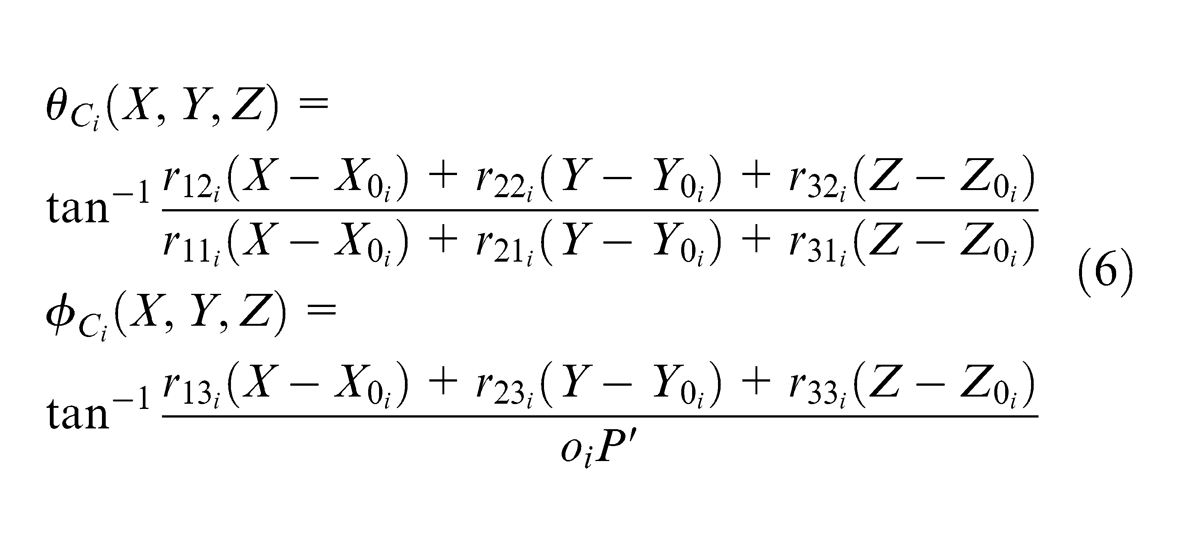
being

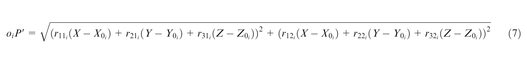
o_{i} P' = \sqrt{{(r_{11_{i}} (X - X_{0_{i}}) + r_{21_{i}} (Y - Y_{0_{i}}) + r_{31_{i}} (Z - Z_{0_{i}}))}^{2} + {(r_{12_{i}} (X - X_{0_{i}}) + r_{22_{i}} (Y - Y_{0_{i}}) + r_{32_{i}} (Z - Z_{0_{i}}))}^{2}}

(7)

Using the two angular local measurements ( $θ_{M_{i}}$ and $ϕ_{M_{i}}$ ) performed by each ith network device, one can set up a system of equations for calculating the three unknown coordinates of P, as

{\begin{cases} {\begin{cases} θ_{M_{1}} = θ_{C_{1}} (X, Y, Z) \\ ϕ_{M_{1}} = ϕ_{C_{1}} (X, Y, Z) \end{cases} \\ {\begin{cases} θ_{M_{2}} = θ_{C_{2}} (X, Y, Z) \\ ϕ_{M_{2}} = ϕ_{C_{2}} (X, Y, Z) \end{cases} \\ \dots \\ {\begin{cases} θ_{M_{N}} = θ_{C_{N}} (X, Y, Z) \\ ϕ_{M_{N}} = ϕ_{C_{N}} (X, Y, Z) \end{cases} \end{cases}

(8)

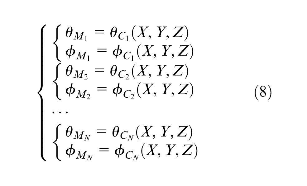
where N is the number of network devices (with a priori known location and orientation) involved in the measurement.

The system in equation (8) can be solved when P is ‘seen’ by at least two devices (2 angles × 2 devices = 4 total equations). Since the triangulation problem is overdefined (more equations than unknown parameters), it can be solved using a minimization approach.¹⁶ The position of P can be estimated by the iterative minimization of a suitable error function (EF). There are many possible choices of the EF to minimize for solving the localization problem. That one in equation (9) was defined trying to keep it as simple and general as possible

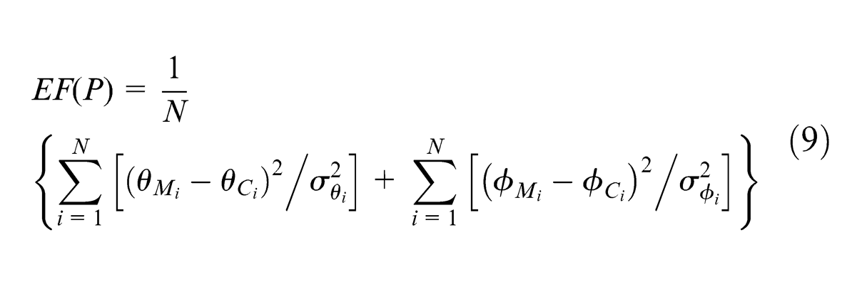
\begin{array}{l} E F (P) = \frac{1}{N} \\ {\sum_{i = 1}^{N} [{(θ_{M_{i}} - θ_{C_{i}})}^{2} / σ_{θ_{i}}^{2}] + \sum_{i = 1}^{N} [{(ϕ_{M_{i}} - ϕ_{C_{i}})}^{2} / σ_{ϕ_{i}}^{2}]} \end{array}

(9)

where P is the point to be localized, whose unknown coordinates (X, Y, Z) are the solution of the problem; $θ_{M_{i}}$ and $ϕ_{M_{i}}$ are the angles locally measured by each ith device (input data of the problem); $θ_{C_{i}}$ and $ϕ_{C_{i}}$ are the angles calculated for each ith device (equation (6)), using the coordinates (X, Y, Z) resulting from the solution of the system. This solution is iterative: each iteration leads to determining an attempt solution, gradually converging to the point of global minimum of the EF. $σ_{θ_{i}}^{2}$ and $σ_{ϕ_{i}}^{2}$ are the (supposed known) variances related to the difference between measured and calculated angles, that is, defined as residuals $(θ_{M_{i}} - θ_{C_{i}})$ and $(ϕ_{M_{i}} - ϕ_{C_{i}})$ . The subscript ‘i’ denotes that these variances are related to each ith device. Since residuals may have different dispersions, they are weighted by the reciprocal of their variance.¹⁷N is the number of network devices involved in the measurement.

It is worth remarking that the determination of the $θ_{M_{i}}$ and $ϕ_{M_{i}}$ values depends on the specific technology of the measuring instrument. For example, in the case of the iGPS, they are determined by the target, measuring the period between the detection of two laser blades emitted by each ith network device.⁶ Besides, for systems based on photogrammetry, such as MScMS-II, they are obtained on the basis of the position of the target in a local image related to the ith network device.⁹

Finally, since the proposed EF is non-linear, its minimization can be computationally expensive. The burden of computation can be eased by employing a suitable linearization technique, for example, techniques based on first-order Taylor expansion, Newton–Raphson method and so on.

The MScMS-II

The MScMS-II is a prototypical measuring instrument, based on infrared (IR) photogrammetric technology. Network devices are low-cost IR cameras associated with IR illuminators, while the hand-held probe has two reflective spheres, whose centres are A and B, and a stylus (V), in contact with the point(s) of interest (see Figure 5). Reflective spheres act as passive targets illuminated by the illuminators. Alternatively, they can be replaced with active spherical targets that emit IR light, not making it necessary to use illuminators.

Figure 5.

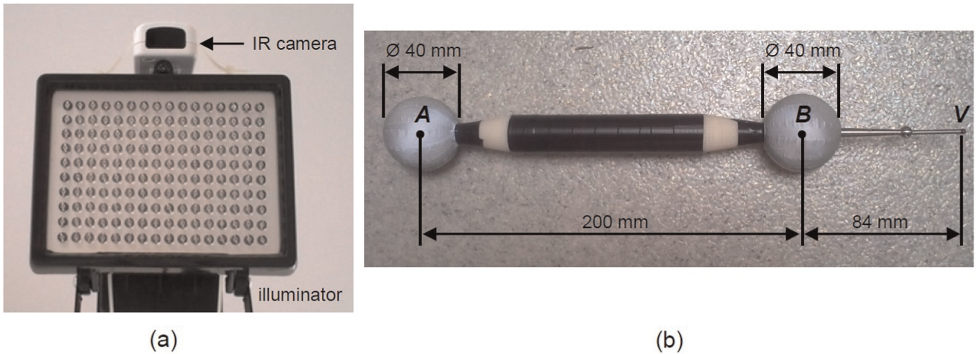
Elementary components of the MScMS-II: (a) IR cameras (acting as network devices) and IR illuminators and (b) hand-held probe with two spherical targets (A and B) and a stylus (V).⁹

The localization of the probe targets allows to uniquely determine the coordinates of the probe stylus, being A, B and V positioned on the same line, at known distances. The measurement uncertainty of MScMS-II for three-dimensional (3D) point coordinates is included within several tenths of a millimetre; for additional details, see Galetto et al.⁹ The hand-held probe was manufactured by a rapid prototyping process, with dimensional error of the order of a few hundredths of a millimetre, that is, at least 1–2 orders of magnitude lower than the measurement uncertainty of MScMS-II. Therefore, the assumption that the spheres and the stylus are exactly on the same line is not unrealistic.

Since A and B have the same diameter, the orientation of V can be ambiguous. However, this problem is overcome by the fact that in the measurement process, the probe is always pointing down (see Figure 1), with sphere A to a higher level with respect to sphere B.

The attention now focuses on each ith network device (camera). Given the position P″≡ (u_i, v_i) of the projection of target P on the camera’s image plane u_iv_i, which is parallel to the plane x_iy_i of the local coordinate system, and knowing some intrinsic parameters of the camera – that is, the focal length (f_i) – it is possible to determine the angles $θ_{M_{i}}$ and $ϕ_{M_{i}}$ (see Figure 6). For more information about (intrinsic and extrinsic) camera parameters, see Galetto et al.⁹

\begin{array}{l} θ_{M_{i}} = {tan}^{- 1} \frac{v_{i} - v_{0_{i}}}{u_{i} - u_{0_{i}}} {\begin{cases} if u_{i} - u_{0_{i}} > 0 then \frac{π}{2} < θ_{M_{i}} < \frac{3 π}{2} \\ if u_{i} - u_{0_{i}} \leq 0 then - \frac{π}{2} \leq θ_{M_{i}} \leq \frac{π}{2} \end{cases} \\ ϕ_{M_{i}} = {tan}^{- 1} \frac{f_{i}}{\sqrt{{(u_{i} - u_{0_{i}})}^{2} + {(v_{i} - v_{0_{i}})}^{2}}} {- \frac{π}{2} \leq ϕ_{M_{i}} \leq \frac{π}{2} \end{array}

(10)

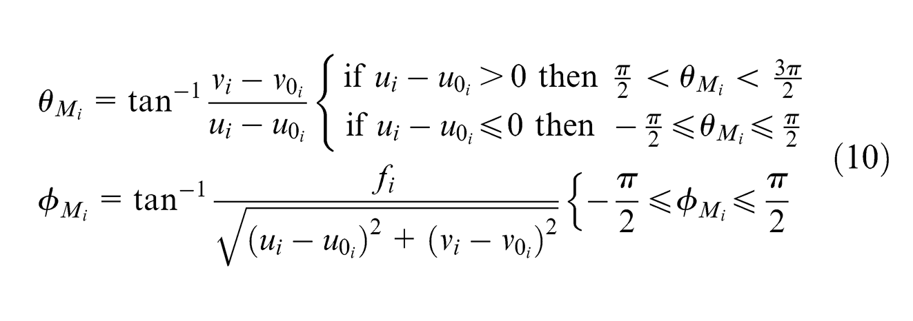
where u_i and v_i are the coordinates of the projection (P″) of P on the image plane; $u_{0_{i}}$ and $v_{0_{i}}$ are the coordinates of the projection of o_i on the plane u_iv_i; f_i is the distance between the plane u_iv_i and the camera projection centre (or focus), which is coincident with the origin o_i of the local coordinate system o_ix_iy_iz_i.

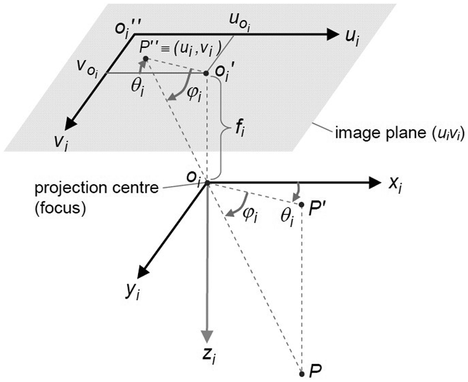
Note that $θ_{M_{i}}$ and $ϕ_{M_{i}}$ are not measured directly: the ‘primary’ quantities, that is, those measured directly by each ith network device, are the coordinates of P″≡ (u_i, v_i). The angles of interest can be then obtained through the formulae in equation (10). Of course, for systems based on other technologies, primary measured quantities may be different.

Figure 6.

For a generic ith network device, representation of the local coordinate system, with origin (o_i) in the projection centre (or focus), and the image plane u_iv_i – parallel to the plane x_iy_i, at a distance f_i (i.e. the focal length).

Angles $θ_{M_{i}}$ and $ϕ_{M_{i}}$ can be compared with $θ_{C_{i}}$ and $ϕ_{C_{i}}$ , that is, those calculated as functions of the (unknowns) coordinates of P (equation (6)), so as to solve the localization problem by the EF minimization (in equation (9)).

Being based upon IR optical technology, MScMS-II is sensible to many influencing factors. The most common measurement accidents are

Vibration or accidental movement of the cameras;

Partial occlusion (e.g. by obstacles interposed between network device(s) and target(s)) or target overlapping;

False targets due to IR light reflection on polished surfaces or the presence of other external uncontrolled IR light sources.

These and other potential causes of accidental measurement errors must be taken under control to assure an acceptable level of accuracy. These aspects are examined in detail in Galetto and Mastrogiacomo.¹⁸

Online diagnostic tests

With the aim of protecting the system, MScMS-II implements some statistical tests for online diagnostics. Three tests are analysed in the following sub-sections:

Test 1: global test on the EF;

Test 2: global test on the distance between probe targets;

Test 3: local test for identifying purportedly faulty device(s).

Test 1: global test on the EF

By definition (see equation (9)), EF(P) ≥ 0 for all the points in the measurement volume $ξ \subseteq ℜ^{3}$ . In particular, EF(P) = 0 when $θ_{M_{i}} = θ_{C_{i}}$ and $ϕ_{M_{i}} = ϕ_{C_{i}}$ , for i = 1 … N. Because of the measurement natural variability, two situations may occur:

EF(P) is strictly positive even in the point of correct localization;

EF(P) converges to a point that is not the correct one. As a result, a local minimum may be confused with the global minimum.

The first diagnostic criterion is aimed at identifying all the non-acceptable minima solutions for EF(P), in order to prevent system fails. Such criterion enables MScMS-II to distinguish between reliable and unreliable measurements.

Let us consider a solution $P \equiv (X, Y, Z)$ to the problem $\min_{P \in ξ} E F (P)$ . In general, being the problem overdetermined (as shown in equation (8)) and since single measurements are affected by noise, a solution that exactly satisfies all angular constrains is not realistically possible. In real conditions, there are two types of residuals: $ε_{θ_{i}} = (θ_{M_{i}} - θ_{C_{i}})$ and $ε_{ϕ_{i}} = (ϕ_{M_{i}} - ϕ_{C_{i}})$ . In the absence of systematic error causes, it is reasonable to hypothesize that they follow two zero-mean normal distributions, that is, $ε_{θ_{i}} ~ N (μ_{θ} \approx 0, σ_{θ_{i}}^{2})$ and $ε_{ϕ_{i}} ~ N (μ_{ϕ} \approx 0, σ_{ϕ_{i}}^{2})$ . These assumptions will be tested empirically.

If $σ_{θ_{i}} = σ_{θ}$ and $σ_{ϕ_{i}} = σ_{ϕ}, \forall i$ (this is true in the absence of spatial/directional effects), equation (9) becomes

E F (P) = \frac{1}{N} \cdot (\sum_{i = 1}^{N} \frac{ε_{θ_{i}}^{2}}{σ_{θ}^{2}} + \sum_{i = 1}^{N} \frac{ε_{ϕ_{i}}^{2}}{σ_{ϕ}^{2}}) = \frac{1}{N} \cdot (\sum_{i = 1}^{N} z_{θ_{i}}^{2} + \sum_{i = 1}^{N} z_{ϕ_{i}}^{2})

(11)

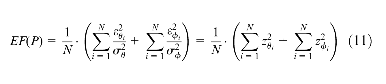
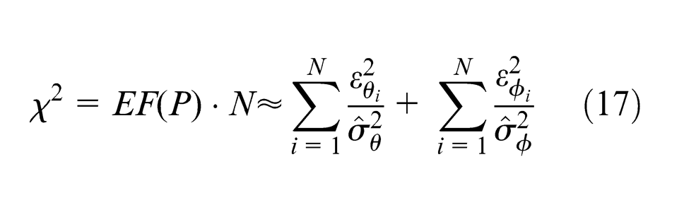
EF(P) can be seen as the sum of the squares of N+N realizations of two series of normally distributed random variables ( $z_{θ_{i}}$ and $z_{ϕ_{i}}$ ) with mean 0 and variance 1, multiplied by the constant term 1/N.

Equation (11) therefore can assume the following form

E F (P) = \frac{1}{N} \cdot (χ_{θ}^{2} + χ_{ϕ}^{2})

(12)

where $χ_{θ}^{2}$ and $χ_{ϕ}^{2}$ are two chi-square distributed random variables, with N degrees of freedom (DOFs) each since they are obtained by the sum of N independent terms; N is the number of network devices involved in the measurement.

The residual standard deviations, that is, σ_θ and σ_ϕ, can be a priori estimated for the whole measurement volume, for example, during the phase of installation and calibration of the system.

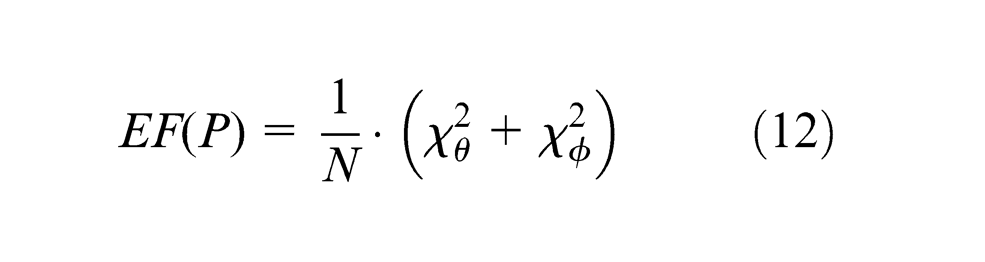
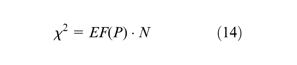
Equation (12) can be expressed as

E F (P) = \frac{1}{N} \cdot χ^{2}

(13)

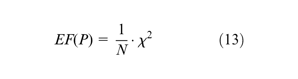
Since χ² is obtained by adding two chi-square distributed variables with N DOF each, it will follow a chi-square distribution with 2·N DOF.¹⁷

Every time the localization of a probe target is performed, MScMS-II diagnostics calculates the following quantity

χ^{2} = E F (P) \cdot N

(14)

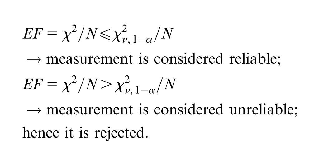
Assuming a risk α as a type I error, a one-sided confidence interval for the variable χ² can be calculated. $χ_{ν, 1 - α}^{2}$ is a chi-square distribution with ν = 2·N DOF and a (1 −α) confidence coefficient. The confidence interval is assumed as the acceptance interval for the reliability test of the measurement.

The test drives to the following two alternative conclusions

\begin{array}{l} E F = χ^{2} / N \leq χ_{ν, 1 - α}^{2} / N \\ \to measurement is considered reliable; \\ E F = χ^{2} / N > χ_{ν, 1 - α}^{2} / N \\ \to measurement is considered unreliable; hence it is rejected . \end{array}

Set-up of test parameters

The risk level α is established by the user. A high α prevents from non-acceptable solutions of the minimization problem, although it might drive to reject good solutions. On the contrary, a low α speeds up the measurement procedure, although it might drive to collect wrong data due to the consequent increase of the type II error β.

The residual standard deviations σ_θ and σ_ϕ can be determined empirically, on the basis of experimental angle measurements. In this case, σ_θ and σ_ϕ are estimated from the residuals obtained by measuring a sample of points randomly distributed in the whole measurement volume $ξ \subseteq ℜ^{3}$ , in the absence of systematic error sources. This operation can be implemented during the initial phase of system set-up and calibration.

Given a set of M points randomly distributed in the measurement volume and measured by a single target (with a random sequence of measurements), two sets of N_j residuals (i.e. $ε_{θ_{i j}}$ and $ε_{ϕ_{i j}}$ ) can be calculated for each jth point (j = 1, …, M, i = 1, …, N_j). The number N_j may change due to the number of network devices involved in each measurement.

In the absence of systematic error causes and time or spatial/directional effects, it is reasonable to hypothesize that $ε_{θ_{i j}}$ and $ε_{ϕ_{i j}}$ are zero-mean normally distributed random variables, that is

\begin{array}{l} ε_{θ_{i j}} = {(θ_{M_{i}} - θ_{C_{i}})}_{j} ~ N (μ_{θ} \approx 0, σ_{θ}^{2}) and \\ ε_{ϕ_{i j}} = {(ϕ_{M_{i}} - ϕ_{C_{i}})}_{j} ~ N (μ_{ϕ} \approx 0, σ_{ϕ}^{2}) \end{array}

(15)

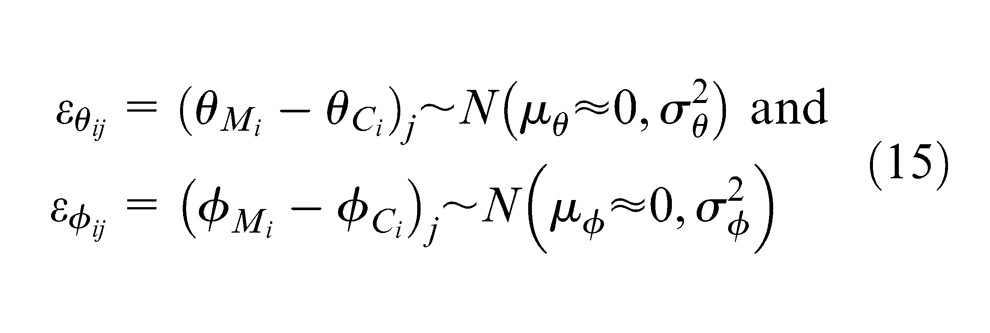
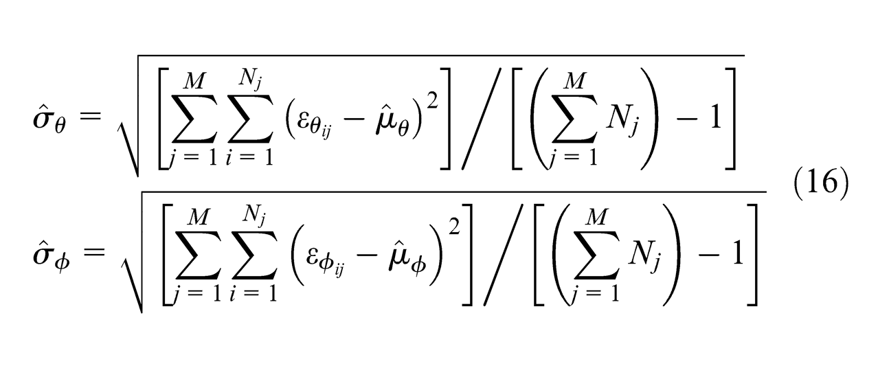
being ${\hat{μ}}_{θ} = (\sum_{j = 1}^{M} \sum_{i = 1}^{N_{j}} ε_{θ_{i j}}) / (\sum_{j = 1}^{M} N_{j}) \approx 0$ and ${\hat{μ}}_{ϕ} = (\sum_{j = 1}^{M} \sum_{i = 1}^{N_{j}} ε_{ϕ_{i j}}) / \sum_{j = 1}^{M} N_{j} \approx 0$ (to be tested).

The standard deviations σ_θ and σ_ϕ may be estimated as follows

\begin{array}{l} {\hat{σ}}_{θ} = \sqrt{[\sum_{j = 1}^{M} \sum_{i = 1}^{N_{j}} {(ε_{θ_{i j}} - {\hat{μ}}_{θ})}^{2}] / [(\sum_{j = 1}^{M} N_{j}) - 1]} \\ {\hat{σ}}_{ϕ} = \sqrt{[\sum_{j = 1}^{M} \sum_{i = 1}^{N_{j}} {(ε_{ϕ_{i j}} - {\hat{μ}}_{ϕ})}^{2}] / [(\sum_{j = 1}^{M} N_{j}) - 1]} \end{array}

(16)

The resulting values of ${\hat{σ}}_{θ}$ and ${\hat{σ}}_{ϕ}$ are used as reference values for the test. With this notation, equation (13) becomes

χ^{2} = E F (P) \cdot N \approx \sum_{i = 1}^{N} \frac{ε_{θ_{i}}^{2}}{{\hat{σ}}_{θ}^{2}} + \sum_{i = 1}^{N} \frac{ε_{ϕ_{i}}^{2}}{{\hat{σ}}_{ϕ}^{2}}

(17)

Experimental example

It was used a network consisting of six cameras (D₁, …, D₆) with known position and orientation, distributed in the measurement volume as schematized in Figure 7. Each camera’s position/orientation is determined through a semi-automated network calibration procedure, illustrated in detail in Svoboda et al.¹⁹ Figure 8 shows an image of the experimental set-up.

Figure 7.

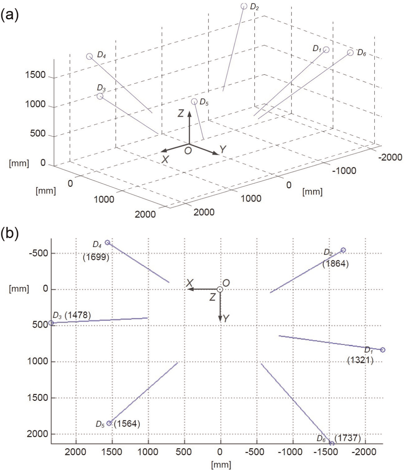
Representation of the positioning and orientation of the MScMS-II network devices used in the application example: (a) 3D view and (b) XY plane view, with Z values relating to the position of each device in parentheses. OXYZ is the global coordinate system (coordinates in millimetres). The measuring volume contains six network cameras (D₁, …, D₆), whose outgoing vectors (in blue) represent their orientation (colours in online).

Figure 8.

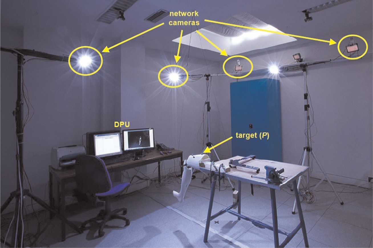
Area of the Industrial Metrology and Quality Engineering Laboratory of DIGEP-Politecnico di Torino, where the experiments were performed.

The standard deviations σ_θ and σ_ϕ were empirically estimated according to the following steps:

M = 290 points distributed in the measurement volume were measured using a single target. The rough position of each point is randomly decided using a random number generator.

The coordinates of each point (P_j, j = 1, …, M) were evaluated by minimizing the EF in equation (9). With respect to $ε_{θ_{i j}}$ and $ε_{ϕ_{i j}}$ , two sets of 1740 and 1740 residuals, respectively, were obtained.

Measurements were performed in a controlled environment (e.g. temperature, light and vibrations were kept under control) and the distributions of residuals were thoroughly analysed, in order to exclude measurement accidents, for example, time or spatial/directional effects, IR light reflection, presence of external IR sources or other non-random causes of variation in general.

The zero-mean normal distribution of each of the two sets of residuals was verified by the Anderson–Darling normality test at p < 0.05.¹⁷

The standard deviations of the two sets of residuals were estimated by equation (16). Table 2 reports the resulting ${\hat{σ}}_{θ}$ and ${\hat{σ}}_{ϕ}$ values and other data concerning them.

Table 2.

Detailed data concerning the estimation of $σ_{θ}$ and $σ_{ϕ}$ (angles in degrees).

Sample size: $N_{T O T} = \sum_{j = 1}^{M} N_{j}$	N_TOT = 1740
Mean value estimates: ${\hat{μ}}_{θ} = (\sum_{j = 1}^{M} \sum_{i = 1}^{N_{j}} ε_{θ_{i j}}) / (\sum_{j = 1}^{M} N_{j})$ and ${\hat{μ}}_{ϕ} = (\sum_{j = 1}^{M} \sum_{i = 1}^{N_{j}} ε_{ϕ_{i j}}) / (\sum_{j = 1}^{M} N_{j})$	${\hat{μ}}_{θ} = 0.301 °$ ; ${\hat{μ}}_{ϕ} = 0.004 °$
Standard deviation estimates: ${\hat{σ}}_{θ} = \sqrt{(\sum_{j = 1}^{M} \sum_{i = 1}^{N_{j}} ε_{θ_{i j}}^{2}) / (\sum_{j = 1}^{M} N_{j} - 1)}$ and ${\hat{σ}}_{ϕ} = \sqrt{(\sum_{j = 1}^{M} \sum_{i = 1}^{N_{j}} ε_{ϕ_{i j}}^{2}) / (\sum_{j = 1}^{M} N_{j} - 1)}$	${\hat{σ}}_{θ} = 0.87 °$ ; ${\hat{σ}}_{ϕ} = 0.06 °$
Maximum: $ε_{θ_{M A X}} = M a x {{ε_{θ}}_{i j} \| i = 1, \dots, N_{j}, j = 1, \dots, M}$ and $ε_{ϕ_{M A X}} = M a x {{ε_{ϕ}}_{i j} \| i = 1, \dots, N_{j}, j = 1, \dots, M}$	$ε_{θ_{M A X}} = 8.30 °$ $ε_{ϕ_{M A X}} = 0.28 °$
Minimum: $ε_{θ_{M I N}} = M i n {{ε_{θ}}_{i j} \| i = 1, \dots, N_{j}, j = 1, \dots, M}$ and $ε_{ϕ_{M I N}} = M i n {{ε_{ϕ}}_{i j} \| i = 1, \dots, N_{j}, j = 1, \dots, M}$	$ε_{θ_{M I N}} = - 11.60 °$ ; $ε_{ϕ_{M I N}} = 0.29 °$ ;

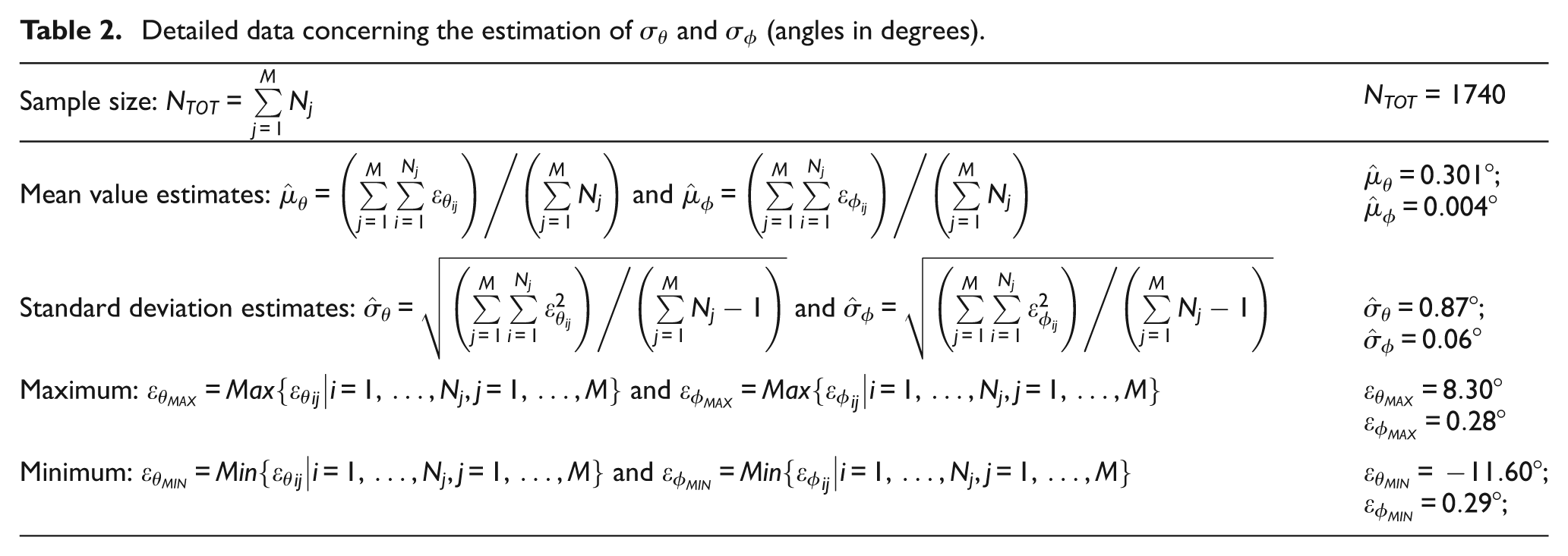
Note that (1) the mean value of both the sets of residuals is roughly zero and (2) the ${\hat{σ}}_{θ}$ value is one order of magnitude higher than the ${\hat{σ}}_{ϕ}$ . The latter behaviour is due to geometric reasons concerning the determination of $θ_{M_{i}}$ and $ϕ_{M_{i}}$ , using the coordinates (u_i, v_i) of the target on one camera’s local image plane (see equation (10)).

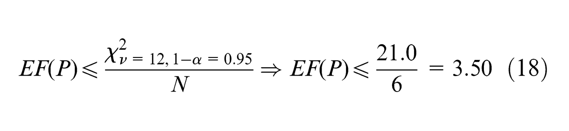
The hypothesis that $ε_{θ_{i j}}$ and $ε_{ϕ_{i j}}$ values have the same standard deviations ( $σ_{θ}$ and $σ_{ϕ}$ ) $\forall_{j} = 1, \dots, M, i = 1, \dots, N_{j}$ as well as the $σ_{θ}$ and $σ_{ϕ}$ estimates may be undermined by particularities regarding the layout of network devices. However, it was observed that when devices are uniformly distributed around the measurement volume, results are not significantly dissimilar, even for different network layouts.

In conditions of maximum visibility (i.e. N = 6 network devices), the acceptance limit for EF, assuming a type I risk level α = 0.05 and ν = 2·N = 2·6 = 12 DOFs, becomes

E F (P) \leq \frac{χ_{ν = 12, 1 - α = 0.95}^{2}}{N} \Rightarrow E F (P) \leq \frac{21.0}{6} = 3.50

(18)

Let us now consider a possible accident that can occur using a MScMS-II or a generic system based on IR photogrammetric technology for locating targets: false targets. Referring to the configuration in Figure 7, suppose that a generic point P inside the measurement volume has to be localized. All the network devices, with the exception of one, that is, D₄, are able to correctly measure the angles ( $θ_{M_{i}}$ and $ϕ_{M_{i}}$ ) subtended by P. An obstacle, for example, an operator who performs the measurement, is interposed between P and D₄, blocking it. At the same time, the IR light reflection on a polished surface within the measurement volume produces a false target (F). This false target is ignored by almost all devices, thanks to a selective technique according to which – in the presence of multiple targets – only those with greater light intensity (P in this case) are regarded as authentic, while others are excluded.

On the contrary, being unable to see P since it is blocked, device D₄ wrongly considers F as a target (see the representation in Figure 9). The consequence is that the angular measurements by D₄ are wrong. See the example in Table 3(a).

Figure 9.

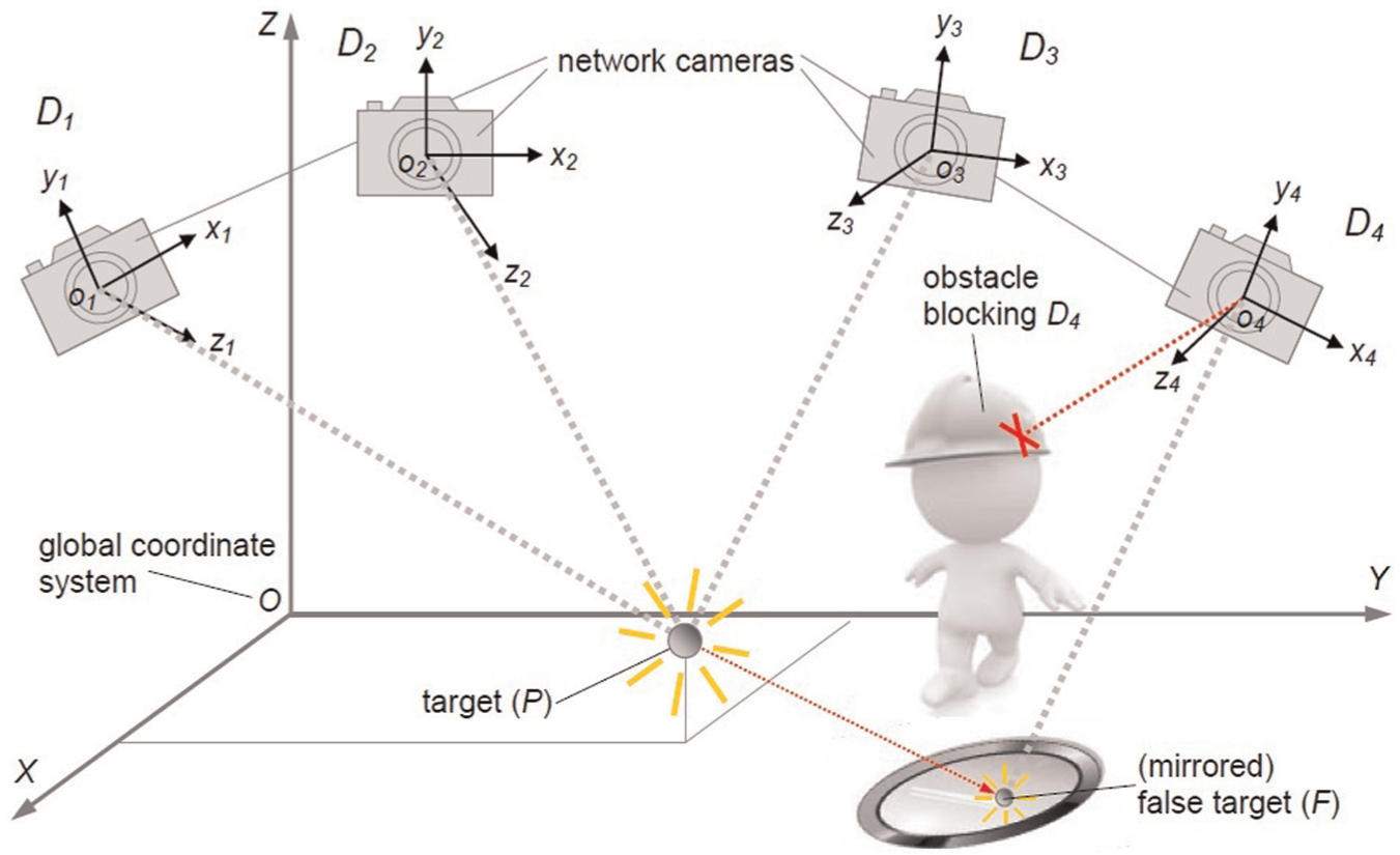
Representation of a possible measurement accident for the MScMS-II: the authentic target P (with high light intensity) is not detected by D₄ because of the interposed obstacle. On the contrary, the false target F– which is ignored by the other cameras because of the low light intensity – is erroneously detected by D₄.

Table 3.

Example of angles measured by the MScMS-II network devices: (a) before and (b) after removing the cause of the measurement accident. Angles are expressed in degrees.

Network device	Measured angles
	(a)		(b)
	$θ_{M_{i}}$	$ϕ_{M_{i}}$	$θ_{M_{i}}^{'}$	$ϕ_{M_{i}}^{'}$
D ₁	28.16°	77.16°	28.25°	77.14°
D ₂	214.39°	76.95°	214.39°	76.9°
D ₃	142.70°	73.34°	142.72°	73.36°
D ₄	(wrong) 311.78°	(wrong) 72.65°	(correct) 304.44°	(correct) 72.96°
D ₅	352.49°	79.86°	352.49°	79.86°
D ₆	185.16°	80.08°	185.16°	80.08°

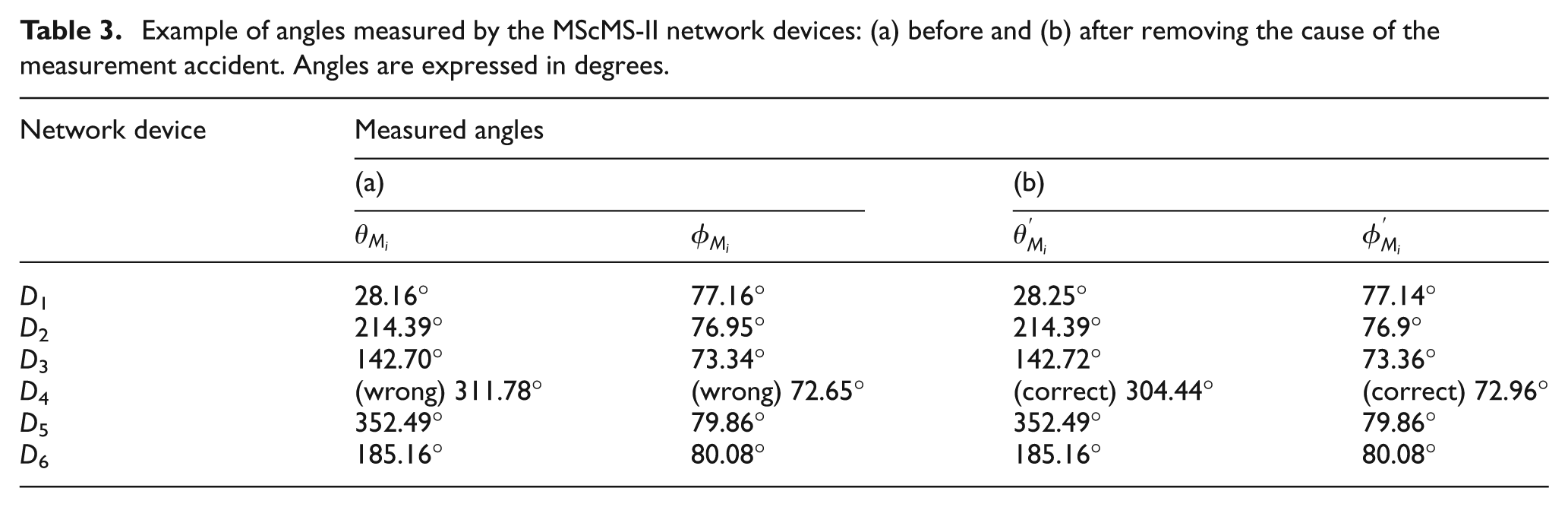
In this case, the algorithm will produce the following wrong localization solution: $P \equiv (104.0, 1062.2, 271.8), (mm)$ , characterized by a high level of error: $E F (P) ≅ 28.02 > 3.50$ . Owing to this result, this diagnostics suggests rejecting the measurement.

After removing the obstacle, the new angles observed by D₄ are $θ_{M_{1}}^{'} = 304.44 °$ and $ϕ_{M_{1}}^{'} = 72.96 °$ , while those relating to the remaining devices are almost identical to the previous ones (see Table 3(b)). The new localization is $P \equiv (85.5, 1035.8, 299.6) (mm)$ . The corresponding EF value is $E F (P) ≅ 2.13 \leq 3.50$ . Hence, the new localization can be considered reliable and the measurement is accepted.

Test 2: global test on the distance between probe targets

As described in Section ‘The MScMS-II’, the hand-held probe is equipped with two targets – that is, A ≡ (X_A, Y_A, Z_A) and B ≡ (X_B, Y_B, Z_B). The distance between the two probe devices (d_AB) is a priori known (see Figure 5(b)). On the contrary, having localized the two targets, their Euclidean distance can be estimated as

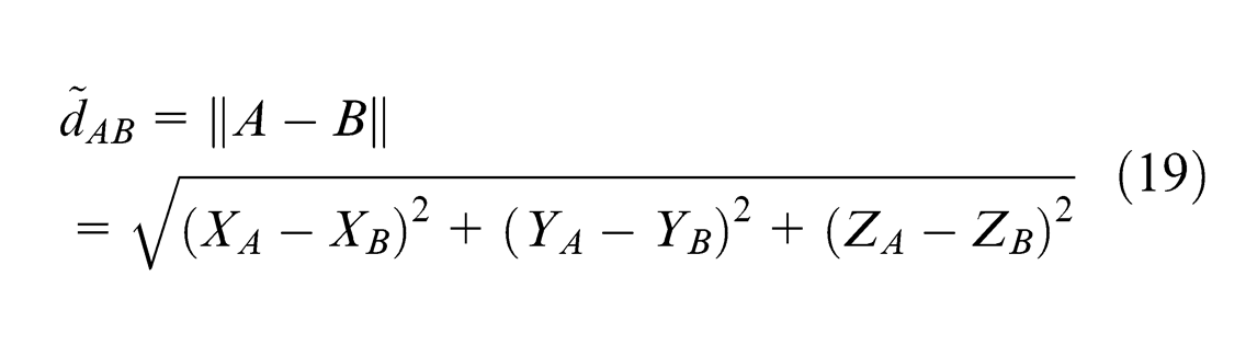
\begin{array}{l} {\tilde{d}}_{A B} = ‖ A - B ‖ \\ = \sqrt{{(X_{A} - X_{B})}^{2} + {(Y_{A} - Y_{B})}^{2} + {(Z_{A} - Z_{B})}^{2}} \end{array}

(19)

The residual ε_AB is defined as

ε_{A B} = {\tilde{d}}_{A B} - d_{A B}

(20)

In the absence of spatial/directional effects, it is reasonable to associate the ε_AB values to a zero-mean normal distribution (this hypothesis will also be tested empirically)

ε_{A B} ~ N (μ_{AB} \approx 0, σ_{A B})

(21)

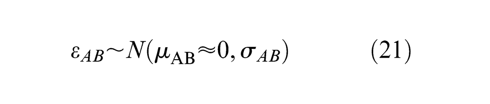
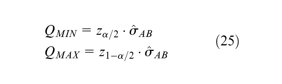
Assuming α as a type I error, a further statistical test can be performed in order to evaluate measurement reliability. Let Q_MIN and Q_MAX be, respectively, the (α/2)-quantile and (1 −α/2)-quantile of a normal distribution with mean µ_AB = 0 and standard deviation σ_AB.

For a given value of α, Q_MIN and Q_MAX can be expressed as multiples of the standard deviation σ_AB

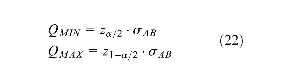
\begin{array}{l} Q_{M I N} = z_{α / 2} \cdot σ_{A B} \\ Q_{M A X} = z_{1 - α / 2} \cdot σ_{A B} \end{array}

(22)

where z_α/₂ and z_(1-α/2) are the α/2- and (1 −α/2)-quantiles of the standard normal distribution. They can be determined by ϕ⁻¹(α/2) and ϕ⁻¹(1 −α/2), respectively, being ϕ⁻¹(Pr) the inverse cumulative distribution function relating to the standard normal distribution.

Again, the σ_AB value can be a priori estimated, during the preliminary stage of the system installation and calibration. Every time a measurement is performed, MScMS-II diagnostics calculates the quantity in equation (20). [Q_MIN, Q_MAX] is assumed as the symmetrical acceptance interval for the measurement reliability test; that is, if the calculated residual ε_AB satisfies the condition

ε_{A B} \in [Q_{M I N}, Q_{M A X}]

(23)

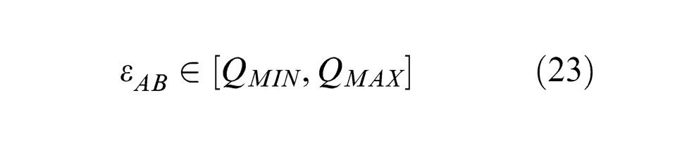
the measurement can be considered reliable, hence it is accepted.

Set-up of test parameters

As usual, the risk level α is established by the user. Similar to the previous diagnostic test (in Section ‘Test 1: global test on the EF’), the standard deviation σ_AB can be evaluated empirically, on the basis of a reasonable number of angular measurements.

A set of M points randomly distributed in the measurement space $ξ \subseteq ℜ^{3}$ are measured according to a random sequence. For each jth measurement (where j = 1, …, M), a residual $ε_{A B, j}$ is calculated.

In the absence of systematic error causes and time or spatial/directional effects, it was hypothesized the same normal distribution for all the random variables $ε_{A B, j}$ , that is, $ε_{A B, j} (μ_{A B}, σ_{A B})$ , being ${\hat{μ}}_{A B} = (\sum_{j = 1}^{M} ε_{A B, j}) / M \approx 0$ (to be tested).

The standard deviation may be estimated as

{\hat{σ}}_{A B} = \sqrt{[\sum_{j = 1}^{M} {(ε_{A B, j} - {\hat{μ}}_{A B})}^{2}] / (M - 1)}

(24)

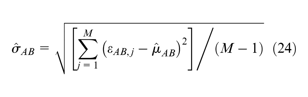
The resulting value of ${\hat{σ}}_{A B}$ is considered as the reference value for the test. Test limits defined in equation (22) become

\begin{array}{l} Q_{M I N} = z_{α / 2} \cdot {\hat{σ}}_{A B} \\ Q_{M A X} = z_{1 - α / 2} \cdot {\hat{σ}}_{A B} \end{array}

(25)

Experimental example

In order to estimate σ_AB, the following steps were followed:

A sample of M = 601 points, randomly measured by the hand-held probe, was considered.

The coordinates of each probe target were evaluated by solving the triangulation problem seen in Section ‘The triangulation problem’, and d_AB is estimated according to equation (19). A sample of 601 residuals ( $ε_{A B, j}$ , j = 1, …, M) was obtained.

The zero-mean normal distribution of residuals was verified by the Anderson–Darling normality test at p < 0.05.

The standard deviation σ_AB was estimated using equation (24). The result is ${\hat{σ}}_{A B} = 0.82 mm$ (see Table 4 for details).

Table 4.

Detailed data concerning the estimation of σ_AB.

Sample size: M	601
Mean estimate: ${\hat{μ}}_{A B} = (\sum_{j = 1}^{M} ε_{A B, j}) / M$	0.97 mm
Standard deviation estimate: ${\hat{σ}}_{A B} = \sqrt{(\sum_{j = 1}^{M} {ε_{A B, j}}^{2}) / (M - 1)}$	0.82 mm
Maximum: $ε_{A B_{M A X}} = M a x {ε_{A B, j} \| j = 1, \dots, M}$	2.60 mm
Minimum: $ε_{A B_{M I N}} = M i n {ε_{A B, j} \| j = 1, \dots, M}$	-2.42 mm

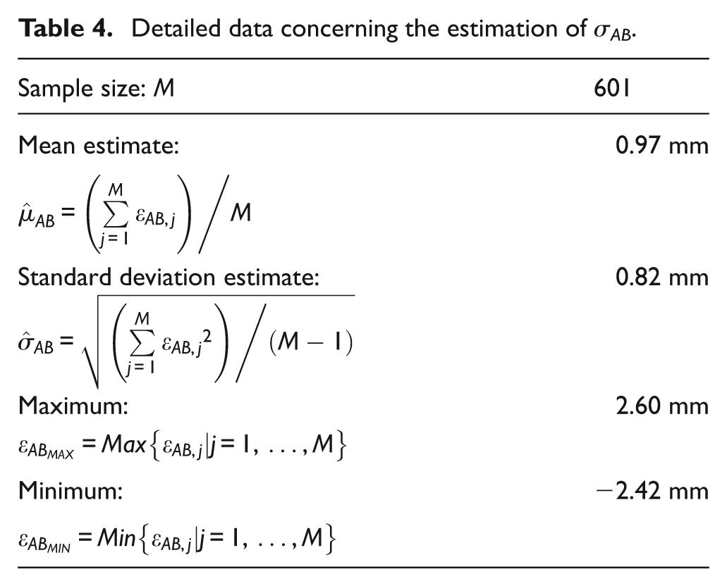
Having assumed α = 5%, the resulting (1 −α) = 95% confidence interval for $ε_{A B}$ is [z_α_/2·σ_AB, z_1-α/2σ_AB] = [−1.96·0.82, 1.96·0.82] = [−1.61, 1.61] mm. A generic measured point cannot be considered unreliable if $‖ ε_{A B} ‖ \leq z_{1 - α / 2} \cdot σ_{A B} = 1.61 mm$ .

Now, considering a measurement similar to that exemplified in Section ‘Experimental example’, let suppose that probe target A is placed on point P. Due to the false-target effect, the localization algorithm produces an incorrect localization of target $A \equiv (90.1, 1026.5, 308.8)$ . Target B’s localization, which is not affected by the false-target error, results in $B \equiv (283.3, 1037.3, 300.1)$ .

The residual concerning the a priori known distance AB is $ε_{A B} = - 6.29 mm$ . This value is not included in the acceptance interval [−1.61; 1.61] mm, hence the system diagnostics automatically suggests to reject the measurement.

After the obstacle is removed, the new coordinates of A become $A \equiv (83.3, 1036.3, 299.6)$ . The new residual is $ε_{A B} = 2.9 \cdot 10^{- 2} mm$ , therefore the new localization is accepted.

Test 3: local test for identifying purportedly faulty device(s)

If at least one of the global tests fails, a local test needs to be performed for failure isolation. The philosophy is to correct the results of a dubious measurement, by excluding the network device(s) that purportedly caused the fault, without losing the observations from the remaining network devices. In this way, the target localization process is never interrupted, even in the presence of local anomalies.

Referring to the measurements carried out by each network device, the two types of residuals defined in Section ‘Test 1: global test on the EF’ can be standardized as

\frac{ε_{θ i}}{σ_{θ}} and \frac{ε_{ϕ i}}{σ_{ϕ}} i = 1, \dots, N

(26)

where $σ_{θ}$ and $σ_{ϕ}$ denote the standard deviations of the residuals related to the θ_i and ϕ_i angles, respectively; N denotes the number of network devices involved in the ith measurement.

The standardized residuals can be used for outlier detection with uncorrelated and normally distributed observations in a sense that if the ith observation is not an outlier, then $ε_{θ_{i}} / σ_{θ}$ and $ε_{ϕ i} / σ_{ϕ}$ are normally distributed $~ N (0, 1)$ . Each standardized residual is compared to a α/2-quantile and a (1 −α/2)-quantile of the standard normal distribution (i.e. z_α_/2 and z_1-α/2), with the significance level α. The null-hypothesis, which denotes that the ith observation is not an outlier, is rejected if at least one of the two standardized residuals in equation (26) is not included in the [z_α_/2, z_1-α/2] symmetrical confidence interval or its absolute value ≤z_1-α/2.

Local testing is easy under the assumption that there is only one purportedly faulty device (or outlier) in the current measurement: the local angular observation with the largest (absolute value of the) standardized residuals, provided that it is beyond the confidence interval, is regarded as an outlier and the corresponding network device (D_i) is excluded from the triangulation problem.

The assumption that there is only one outlier is a severe restriction in the case measurements from more than one network devices are degraded. However, the procedure can be extended to multiple outliers iteratively: after exclusion of a potentially faulty device, the statistical test and the rejection of one other device can be repeated for that epoch until no more outliers are identified.¹³ Of course, assessment for such multiple outliers may give rise to extensive computations. However, they represent a very rare event.

Set-up of test parameters

The parameters $σ_{θ}$ and $σ_{ϕ}$ in equation (26) are the same as used in the (global) Test 1; therefore see Section ‘Set-up of test parameters’.

Application example

Returning to the example presented in Section ‘Experimental example’ (in which device D₄ detects a false target), the relevant normalized residuals are reported in Table 5(a).

Table 5.

Standardized residuals for the measurement exemplified in Section ‘Experimental example’: (a) before and (b) after the exclusion of the observations from D₄.

Network device	Standardized residuals
	(a)	(b)
D ₁	$ε_{θ_{1}} / {\hat{σ}}_{θ} = - 0.59 and ε_{ϕ_{1}} / {\hat{σ}}_{ϕ} = 3.11$	$ε_{θ_{1}} / {\hat{σ}}_{θ} = - 0.51 and ε_{ϕ_{1}} / {\hat{σ}}_{ϕ} = 1.94$
D ₂	$ε_{θ_{2}} / {\hat{σ}}_{θ} = - 0.69 and ε_{ϕ_{2}} / {\hat{σ}}_{ϕ} = 0.56$	$ε_{θ_{2}} / {\hat{σ}}_{θ} = - 0.35 and ε_{ϕ_{2}} / {\hat{σ}}_{ϕ} = - 0.01$
D ₃	$ε_{θ_{3}} / {\hat{σ}}_{θ} = - 0.10 and ε_{ϕ_{3}} / {\hat{σ}}_{ϕ} = 1.55$	$ε_{θ_{3}} / {\hat{σ}}_{θ} = 0.22 and ε_{ϕ_{3}} / {\hat{σ}}_{ϕ} = 0.82$
D ₄	$ε_{θ_{4}} / {\hat{σ}}_{θ} = 7.26 and ε_{ϕ_{4}} / {\hat{σ}}_{ϕ} = - 6.16$	(excluded)
D ₅	$ε_{θ_{5}} / {\hat{σ}}_{θ} = - 0.79 and ε_{ϕ_{5}} / {\hat{σ}}_{ϕ} = - 0.53$	$ε_{θ_{5}} / {\hat{σ}}_{θ} = - 0.27 and ε_{ϕ_{5}} / {\hat{σ}}_{ϕ} = 0.04$
D ₆	$ε_{θ_{6}} / {\hat{σ}}_{θ} = 0.96 and ε_{ϕ_{6}} / {\hat{σ}}_{ϕ} = - 1.53$	$ε_{θ_{6}} / {\hat{σ}}_{θ} = - 0.88 and ε_{ϕ_{6}} / {\hat{σ}}_{ϕ} = - 0.45$

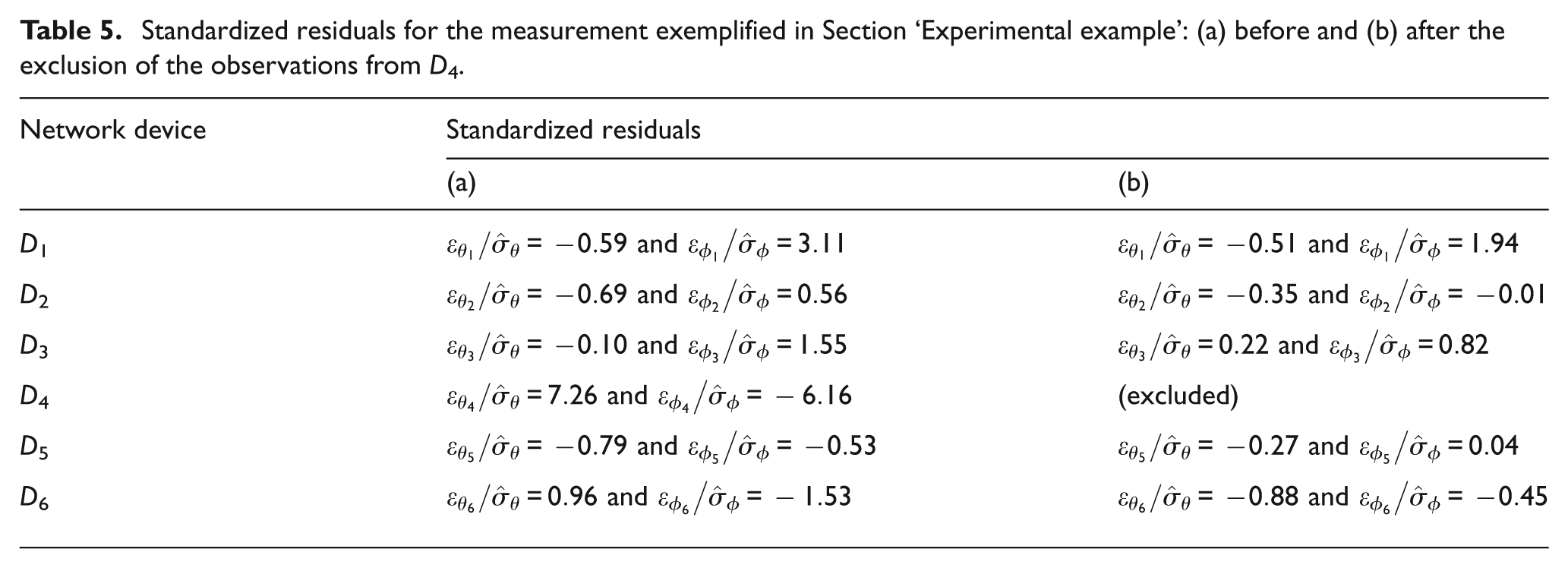
In this calculation, the ${\hat{σ}}_{θ}$ and ${\hat{σ}}_{ϕ}$ values previously estimated were used. Assuming α = 5%, the confidence interval is [z_α_/2 = −1.96, z_1-α/2 = 1.96]. More than one residual is outside this interval – that is, both the residuals of D₄ and one of D₁– but the ‘prime suspect’ is D₄, being the device with the highest (absolute) values of residuals.

D₄ is then excluded and, repeating the localization, the new output is (83.2, 1036.5, 299.5) (mm). All the standardized residuals are now contained within the confidence interval (see Table 5(b)).

Not surprisingly, the Test 1 – performed using only the observations from the five remaining devices – is satisfied; precisely, $E F (P) = 2.20 \leq χ_{ν = 10, 1 - α = 0.95}^{2} / 5 ≅ 3.66$ .

Implications, limitations and future research

The online diagnostics presented in the article make it possible to monitor measurement reliability in real time, on the basis of some statistical tests. Although tests were implemented on MScMS-II, they are deliberately general and can be applied to any distributed LSDM system based on triangulation (e.g. iGPS and HiBall).

An important characteristic of these tests is their ability to selectively exclude faulty network device(s), without interrupting the measurement process. In addition to these tests, note that MScMS-II implements other tests, specifically related to photogrammetric technology (e.g. tests concerning epipolar geometry), which were deliberately ignored in this article. For more information, see Svoboda et al.¹⁹ and Luhmann et al.²⁰

The tests described in this article require the estimation of some parameters, primarily the standard deviations related to the measurement residuals. These parameters can be evaluated empirically by performing some preliminary measurements under controlled conditions, according to the reasonable assumption of the absence of time or spatial/directional effects. This operation can be performed during the system set-up and calibration, with no additional effort.²¹

Since the online implementation of these tests requires a certain computational capacity, it could slow down the measurement process. However, this consequence is minimized due to (1) the high capacity of existing processors and (2) test segmentation (i.e. local Test 3 is performed only after at least one of the global Tests 1 and 2 has detected the presence of potential anomalies). Also, a reduction of the computational workload can be achieved by linearizing the EF.

Finally, it should be remarked that in (global) Test 2, it was considered a hand-held probe with two targets. However, it may be extended to probes with multiple targets (i.e. the so-called 6-DOF probes): in this case, there would be multiple a priori known distances.⁷

Future development of this research will be aimed at developing other diagnostic models for dynamic measurements (e.g. mobile object tracking). One possibility may be the integration of the models presented in this article with techniques based on the Kalman filtering.¹⁸

Footnotes

Declaration of conflicting interests

The authors declare that there is no conflict of interest.

Funding

This research received no specific grant from any funding agency in the public, commercial or not-for-profit sectors.

References

Franceschini

Galetto

Maisano

. Distributed large-scale dimensional metrology. London: Springer, 2011.

Estler

Edmundson

Peggs

. Large-scale metrology – an update. CIRP Ann-Manuf Techn 2002; 51: 587–609.

Peggs

Maropoulos

Hughes

. Recent developments in large-scale dimensional metrology. Proc IMechE, Part B: J Engineering Manufacture 2009; 223(6): 571–595.

Puttock

. Large-scale metrology. CIRP Ann-Manuf Techn 1978; 21(1): 351–356.

Cuypers

Van Gestel

Voet

. Optical measurement techniques for mobile and large-scale dimensional metrology. Opt Laser Eng 2009; 47(3–4): 292–300.

Maisano

Jamshidi

Franceschini

. Indoor GPS: system functionality and initial performance evaluation. Int J Manuf Res 2008; 3(3): 335–349.

Welch

Bishop

Vicci

. High-performance widearea optical tracking the HiBall tracking system. Presence-Teleop Virt 2001; 10(1): 1–21.

NPL, http://www.npl.co.uk/news/npl-launches-portable-co-ordinate-measurement-systems-training-to-meet-industry-demands (2013).

Galetto

Mastrogiacomo

Pralio

. MScMS-II: an innovative IR-based indoor coordinate measuring system for large-scale metrology applications. Int J Adv Manuf Tech 2011; 52(1–4): 291–302.

10.

Butler

. An investigation into the performance of probes on coordinate measuring machines. Ind Metrol 1991; 2(1): 59–70.

11.

JCGM 200:2008. VIM–international vocabulary of metrology–basic and general concepts and associated terms (VIM). Geneva: International Organization for Standardization, 2008.

12.

Gertler

. Fault detection and diagnosis in engineering system. New York: Marcel Dekker, 1998.

13.

Wieser

Petovello

Lachapelle

. Failure scenarios to be considered with kinematic high precision relative GNSS positioning. In: Proceedings of the ION GNSS 2004, Long Beach, CA, 21–24 September 2004, pp. 1448–1459.

14.

Franceschini

Galetto

Maisano

. On-line diagnostics in the Mobile Spatial coordinate Measuring System (MScMS). Precis Eng 2009; 33(4): 408–417.

15.

Hartley

Zisserman

. Multiple view geometry in computer vision. 2nd ed. Cambridge: Cambridge University Press, 2003.

16.

Wolberg

. Data analysis using the method of least squares: extracting the most information from experiments. Heidelberg: Springer Verlag, 2005.

17.

Box

GEP

Hunter

. Statistics for experimenters. New York: Wiley, 1978.

18.

Galetto

Mastrogiacomo

. Corrective algorithms for measurement improvement in MScMS-II (Mobile Spatial coordinate Measurement System). Precis Eng 2013; 37(1): 228–234.

19.

Svoboda

Martinec

Pajdla

. A convenient multi-camera self-calibration for virtual environments. Presence-Teleop Virt 2005; 14(4): 407–422.

20.

Luhmann

Robson

Kyle

. Close range photogrammetry principles, methods and applications. Caithness: Whittles Publishing, 2006.

21.

Bar-Shalom

Kirubarajan

Estimation with applications to tracking and navigation. New York: Wiley, 2001.

Cooperative diagnostics for distributed large-scale dimensional metrology systems based on triangulation

Abstract

Keywords

Introduction and literature review

Background information

Basic concepts concerning diagnostics

The triangulation problem

The MScMS-II

Online diagnostic tests

Test 1: global test on the EF

Set-up of test parameters

Experimental example

Test 2: global test on the distance between probe targets

Set-up of test parameters

Experimental example

Test 3: local test for identifying purportedly faulty device(s)

Set-up of test parameters

Application example

Implications, limitations and future research

Footnotes

Declaration of conflicting interests

Funding

References