Sage Journals: Discover world-class research

Abstract

The characteristics of the semiconductor industry are short product life cycle, lumpy demand, long lead time, and so on. Theory of constraint suggests a simple replenishment policy to effectively manage supply chain inventory by a demand-pull approach combined with buffer management. However, a demand-pull approach sometimes causes out of stock when the products have lumpy demand. In order to effectively solve this issue, this article integrated market demand forecast information and demand-pull replenishment to improve the inventory management effectiveness of wafer fabrication. An integrated circuit design house provides actual demand per week and market forecast information to the wafer fab. Wafer fab uses inventory buffer to meet customer demand and adjust inventory quantity according to market forecast information and demand-pull replenishment policy. A case of a wafer product that has been drawn from a professional wafer foundry company located in Taiwan is presented to further illustrate the proposed approach. After comparing the result that was obtained from the proposed approach with the traditional demand-pull method, it was found that the proposed approach helps keep high service levels and avoid being out of stock.

Keywords

Inventory management demand-pull replenishment theory of constraint buffer management market demand forecast

Introduction

Under the influence of the trend of globalization, there is an increasingly close cooperation between enterprises. Influence between the raw material supplier, manufacturer, wholesaler, and retailer in the process of raw materials to end items has been deeper for each other. Therefore, a business should consider the internal profit and must pursue profit maximization of the supply chain. From the perspective of the supply chain, when an end customer purchases a product, the demand order information transmits from downstream retailer to upstream raw material suppliers. This shows that the demand information is critical factor in supply chain. However, information transfer delays and alterations will cause the demand variation to be progressively larger in the process of pass messages, called the bullwhip effect. In order to avoid being out of stock, every member will keep enough safety stock for demand variation and uncertainty.

Holding enough inventories can avoid being out of stock, but too many inventories will cause the problem of a backlog of funds and excess inventory costs, becoming a burden on the entire supply chain. The main products of the semiconductor supply chain for an integrated circuit (IC) and its manufacturing process are quite complex and involve cooperation between members of the supply chain. The IC production process mainly includes the following five stages: IC design, wafer fabrication, wafer probing, assembly, and final test. Figure 1 shows the production process of the semiconductor supply chain.

Figure 1.

Production process of the semiconductor supply chain.

In the traditional supply chain collaboration model, IC design companies usually estimate the annual market demand and advance notice to a wafer fab to retain their capacity, arrange production schedule planning, and then place an order with the wafer fab according to the actual market situation. After completed production, the wafer fab will be transported to an assembly and testing company according to the requirements of IC design companies. This process needs to be upstream and downstream of the supply chain for closer cooperation and integration to let the whole supply chain have a strong competitive advantage. However, IC design companies face short product life cycles, long lead time, lack of capacity, and so on. These factors are likely resulting in out-of-stock supply chains and thus the loss of sales opportunities. Therefore, IC design companies may inflate demand to ensure the wafer fab capacity. In this way, it will cause a wafer fab to bear the risk of overcapacity and idle machines. On the other hand, market demand variation generates trouble. IC design companies will continue to submit a large number of orders when the market demand surges and will cause the delayed wafer fab delivery. When market demand declines, the IC design companies are unwilling to burden inventory, causing delayed wafer fab pickup. Therefore, wafer fabs will manufacture according to own experience and capacity rather than orders.

The past practice of the wafer fab is based on demand forecasts to determine the production quantity. However, it will cause the inventory to be too high or out of stock of wafer fabs because of inaccurate forecasts. In order to pursue profit maximization of the semiconductor supply chain, Goldratt and Cox¹ first proposed the concept of theory of constraints (TOC); they believe that every enterprise has its own pursuit of the goal. The idea of TOC is to “break through the key bottlenecks to maximize efficiency.” Many works applied TOC to probe the related issues of the semiconductor supply chain, such as that by Wu et al.,² who proposed an enhanced simulation model for a TOC supply chain replenishment system under capacity constraint. The enhanced model is developed on the basis of minimum capacity loss and minimum replenishment quantity. Therefore, the enterprise can find out suitable adjusting buffer times, revising ratios with different product properties and industries when the strategy actually applies. Hung et al.³ constructed a decision support system to assist decision makers to determine appropriate parameters when using demand-pull replenishment policy. Tyan et al.⁴ applied TOC to develop a state-dependent dispatch rule to improve multisystem performances with fixed station resources in wafer fabrication. Furthermore, Hsieh and Hou⁵ proposed a production-flow-value-based job dispatching rule by the TOC for wafer fabrication. This study derives a TOC cost estimation method to estimate the cost of the work-in-process wafer. Due to its simple yet robust methodology, a great deal of the academic literature^6–8 has focussed on TOC methods.

When enterprises face uncertainty in the future, they usually use forecast to assess the results. They hope to draw up plans from uncertainty forecasts to lower risk in the future. The concept, using the latest information to revise forecasts by time advancing to increase the accuracy rate of forecasts, is called rolling forecast. Rolling forecast can modify forecasts by market information and promote the reactive capability of enterprises for customer demand. Perry and Sohal⁹ thought that one significant function of sharing forecast and sales data is that the upstream and downstream in a supply chain can communicate more closely.

Many studies explored the issue of replenishment planning and safety stock in the past. Dellaert and Jeunet¹⁰ provided an alternative repair procedure to safety stock policies for a multilevel rolling schedule problem. Jeunet¹¹ thought that actual demand is uncertain and assumed that forecast error is a normal distribution. The forecast error is increasing with time; in other words, if forecast period is farther than the current period, the forecast error is greater. However, no analysis was given to study the effect of market demand forecast information on the inventory management of wafer fabrication. Therefore, this article proposed a novel replenishment model—integrated market demand forecast (offered by customer) and demand-pull replenishment policy—to improve the inventory management effectiveness of wafer fabrication. Moreover, this article also simulated and compared the results for demand-pull replenishment using and not using market forecast information according to different demand patterns and different forecast errors.

The remaining article is organized as follows: In section “Literature review,” traditional replenishment policy, supply chain coordination, and TOC are presented and discussed. Section “Methodology” presents the proposed approach, which integrates market demand forecast and demand-pull replenishment to improve the inventory management effectiveness of wafer fabrication. A real case of a wafer product is adopted and different demand patterns are simulated; then, this article compares the differences of average stock and service levels between demand-pull with market forecast information and original demand-pull policy in section “Case study.” Finally, Section “Conclusion” concludes this article.

Literature review

Replenishment policy

In the past, most companies used (s, Q), (s, S), (R, S), and (R, s, S) replenishment policies to maintain inventory levels to meet customer demand.

(s, S) policy

When the inventory position is less than or equal to the reorder point (s), then ask for replenishment to bring it up to the upper limit S. However, the replenishment quantity is variable per period; it is easy to increase the upstream fluctuations in demand. In this policy, the reorder point (s) and upper limit (S) are key factors of replenishment policy. Many studies reviewed reorder point (s) and upper limit (S) in the past, such as Archibald and Silver,¹² who developed recursive formulae to calculate the cost for any pair (s, S) and determine the optimal s and S. Mak et al.¹³ proposed the analysis of optimal opportunistic replenishment policies for inventory systems using a (s, S) model with a maximum issue quantity restriction to avoid being out of stock.

(s, Q) policy

When inventory position is less than the reorder point (s) in any time, then ask for replenishment; the replenishment quantity is Q. This policy is easy to understand and operate, and demand is more stable for an upstream factory. But in case of huge demand variation, it cannot respond instantly. Natarajan and Goyal¹⁴ reported the minimum total expected cost to determine the safety stock and Q and discussed how to set safety stock and interpreted a correlation between s and Q.

(R, S) policy

It checks inventory level at a fixed period R and asks for replenishment to bring it up to the upper limit S. Although it is easy to operate, it is easy to cause out-of-stock conditions when total demand is larger than the upper limit S at period R.

(R, s, S) policy

This policy is mixed by (s, S) and (R, S). It checks inventory level at a fixed period R; if the inventory position is less than the reorder point (s), then ask for replenishment to bring it up to the upper limit S; if inventory position is more than the reorder point (s), then check inventory position after next period R. A number of works in the literature^15–17 have been carried out searching for the optimal parameters. Babai et al.¹⁸ compared heuristic search methods by a practical case of an electronic manufacturing company and found that the search method proposed by Naddor¹⁷ was able to minimize the total cost.

Supply chain coordination

Currently, working on the supply chain coordination between supplier and manufacturer has progressed rapidly. The critical issue of the supply chain is the coordination between a manufacturing firm and its supplier. In order to sustain the partnership between supplier and manufacturers, the coordination should enhance the profitability of not only the manufacturer, but also the suppliers.¹⁹ Barbarosoglu²⁰ developed a decision support tool that can be used by a supplier in making realistic production, sales, and price decisions in a supply chain environment. The main emphasis on buyer purchasing requisition cost should be shared by the buyers and the supplier to satisfy supplier profit and buyer cost reduction expectations simultaneously. Kayis et al.²¹ have proven that the vertical integration of the tier 1 and 2 suppliers will increase the manufacturer’s expected profit. Li et al.²² proposed a dynamic contract problem for managing critical suppliers using business volume incentives to explore a repeated game between a manufacturer and two competing suppliers. They used a performance-based contract to deal with the contract design between supplier and manufacturers. Supply chain partnership implies that the raw material supplier, manufacturer, wholesaler, and retailer need to combine their information to form a single shared demand forecast to pursue profit maximization of the supply chain.^23–24

TOC was proposed by Goldratt and Cox.¹ We believe that every enterprise has its own pursuit of the goal. Every system has at least one constraint factor, called the bottleneck. This concept of TOC is to “break through the key bottlenecks to maximize efficiency.” Enterprises should utilize limited resources in the most important position to eliminate the system constraint factors and optimize benefit.

TOC believes that conflicts exist in enterprises from a supply chain and distribution perspective. The supply chain should achieve the lowest cost or total inventory level to successfully execute inventory management and sell most products as much as possible to obtain the largest profit. However, achieving the lowest cost or total inventory level requires one to prepare a smaller inventory; but, to sell maximum of a product or to avoid out-of-stock situations a bigger inventory is needed—a conflict happens. Goldratt and Cox¹ believe that most people have the wrong intuition to look for a way to compromise when a conflict happens. But a compromise cannot achieve the objective and instead diverges from the original objective. Therefore, a good solution should find the assumption behind the conflict and break the assumption to bring up the win–win solution.²⁵

Demand-pull replenishment

In terms of supply instability, Goldratt and Cox¹ believed that large order quantities and production are major reasons of elongated replenishment cycles and cause supply instability. Therefore, they proposed that “lower lot size” and “increase (of) replenishment frequency” shorten lead time and lower total inventory. This practice is a challenge of management conception for suppliers who are accustomed to large product lot sizes and pursue high capacity. In fact, increase of the replenishment frequency will cause raised in-transit stock and relative on-hand inventory reduction.

Fisher et al.²⁶ thought that the demands are more close to the upstream and the total forecast error will be lower and more accurate. Therefore, the inventory should be placed where demand collection is as far as possible in the midstream or upstream suppliers in the supply chain. Regional warehouses or retailers only need to prepare adequate inventories to meet demand in lead time. Furthermore, a supply chain should change operating models from push based to pull based. The downstream places an order with the upstream according to the number of actual sales. Upstream adjusts according to the actual demand of downstream to production and maintains the appropriate inventory.

When a customer purchases a product, the retailer places an order to the distributor according to the buffer consumption per period, and the distributor uses established buffer shipments to retailers and places an order with the supplier according to the number of actual sales. Then, the supplier provides inventory to the distributor and production according to the consumption of inventories per period. It can reduce the lead time.

Buffer management

In addition to the demand-pull replenishment policy, TOC provides buffer management to respond to long-term demand variation. Buffer management refers to the members of the supply chain to establish an inventory buffer and uses the inventory buffer to meet customer demand. Per period is in accordance with the concept “demand quantity is equal to replenishment quantity” for replenishment. It divides buffers into red (rush), yellow (warning), and green (neglect) zones; each zone is one-third of a buffer. It indicates a different inventory status and periodically monitors the inventory level. When inventory level is in the red zone for a long time, it means the buffer is too low and will be out of stock easily; one should rush or raise the buffer. When inventory level is in the yellow zone, one should replenish normally and monitor continuously, and when inventory level is in the green zone for a long time, it means that inventory is sufficient and the buffer may be too high; one should decrease the buffer. Buffer management can keep inventory at a fit level without going out of stock.²⁵

Buffer management has three important decision parameters: (1) the size of the initial inventory buffer, (2) timing for adjusting the buffer, and (3) size for adjusting the buffer. The diagram of demand-pull with buffer management is shown in Figure 2.

Figure 2.

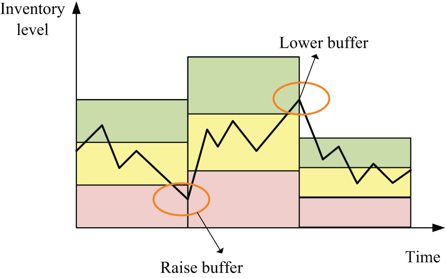
Diagram of demand-pull with buffer management.

Throughput-dollar-days

When the company or department is out of stock, the company’s credit is impaired, and the damage is greater with a long out-of-stock period. Hence, throughput-dollar-days (TDD) surveys the performance of replenishment policy from a reliability point of view. When the company or department due date of promised delivery cannot be reached, counting TDD expresses the degree of customer dissatisfaction. The computing formula is value of throughput × number of delayed days.

Inventory-dollar-days

When the company or department begins to accumulate inventories, it also begins to generate related cost. Hence, inventory-dollar-days (IDD) represents a measure of the inventory level of the company or department from an efficiency point of view. When the inventories begin to accumulate, counting IDD expresses the efficiency of a company. The computing formula is value of inventory × total residence time that inventory is parked in the warehouse.

Methodology

Difficulty of replenishment management arises because of characteristics, such as short life cycle, large demand variation, and long lead time in the semiconductor industry. This article suggests that the wafer fabrication factory uses market forecast information of demand-pull replenishment to manage supply chain inventory. IC design companies provide actual weekly demand and market forecast information for the next few weeks to the wafer fabrication factory. Wafer fabrication factories calculate the lead time of expected inventory according to the actual weekly demand and market forecast information. If replenishment was in total accordance with forecast, they may be out of stock because of an incorrect forecast. Demand-pull replenishment can effectively reduce inventory and shorten replenishment time, but they may be out of stock when facing a larger demand variation. Then, integrating market demand forecast information and demand-pull replenishment can maintain a certain service level and avoid being out of stock.

Demand-pull replenishment

Demand-pull replenishment policy constructs a buffer to meet customer demand in a warehouse at the initial period, and customers actually demand consumption as the replenishment quantity. In an unadjusted buffer situation, the buffer (in-transit inventory + inventory) is fixed. In this model, the ith buffer T_i is expressed as follows

T_{i} = S R_{i} + O H_{i}

(1)

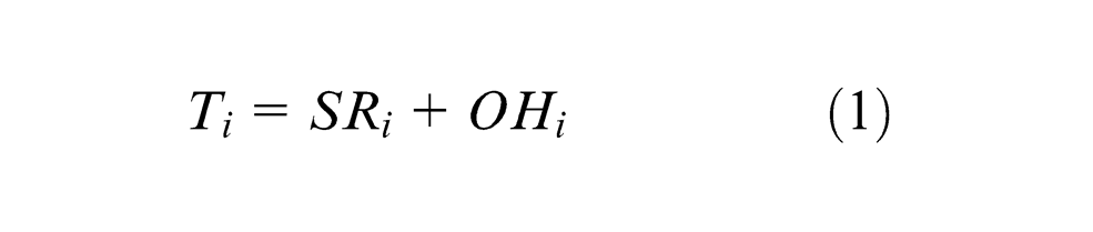
SR_i expresses the in-transit inventory, and OH_i is the inventory level in the ith period. The inventory level formula is

O H_{i} = O H_{i - 1} + F G_{i} - D_{i}

(2)

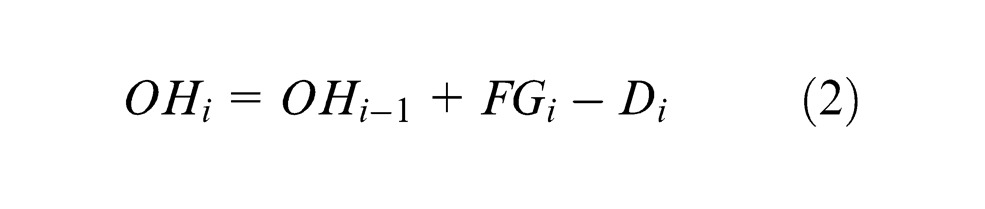
FG_i is quantity received, and D_i expresses actual demand.

Demand-pull replenishment policy coordination buffers management to adjust the buffer: divide buffer into red, yellow, and green zones. According to state records of the inventory level (OH_i), consecutive phases are located in the red zone (r_i) or green zone (g_i). Then, based on the preset, adjust the number and ratio to adjust inventory buffer. Related parameters are defined in the following.

r: red zone reactor, r ∈ N

Red zone reactor (r) is used to record and assess timing of raising the buffer. While inventory level is in the red zone for r periods continuously, it indicates that it was the timing of raising the buffer.

g: green zone reactor, g ∈ N

Green zone reactor (g) is used to record and assess the timing of lowering the buffer. While inventory level is in the green zone for g periods continuously, it indicates that it was the timing of lowering the buffer.

IT: enlarge proportion, IT ∈ R+

Enlarge proportion (IT) is used to represent that the margin of buffer requires raising. While inventory level is the timing of raising the buffer, buffer rises to 1 +IT times.

DT: reduce proportion, DT ∈ R+

Reduce proportion (DT) is used to represent that the margin of buffer requires lowering. While inventory level is the timing of lowering the buffer, buffer lowers to 1 -DT times.

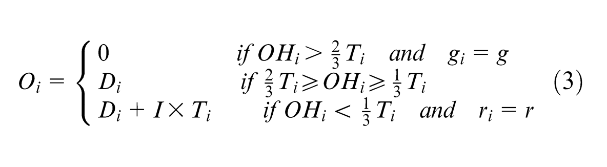
When inventory level (OH_i) is continuous in the red zone (r_i) to reach the red zone reactor (r), then raise buffer and replenishment quantity; if inventory level is in the yellow zone, then replenishment is accordance with customer consumption. While inventory level (OH_i) is continuous in the green zone (g_i) to reach the green zone reactor (g), then lower the buffer and stop replenishment.

Synthesizing the above description, replenishment quantity of period ith, O_i can be expressed as

O_{i} = {\begin{array}{l} 0 & i f O H_{i} > \frac{2}{3} T_{i} a n d g_{i} = g \\ D_{i} & i f \frac{2}{3} T_{i} \geq O H_{i} \geq \frac{1}{3} T_{i} \\ D_{i} + I \times T_{i} & i f O H_{i} < \frac{1}{3} T_{i} a n d r_{i} = r \end{array}

(3)

Integrate market forecast information and demand-pull replenishment

This article constructs a demand-pull replenishment policy with market forecast information for large demand variation and long lead time product. Customer uses actual consumption and weekly market forecast information for future periods delivered to the warehouse. The warehouse uses the inventory buffer to meet customer needs and decide replenishment quantity according to market forecast information and demand-pull replenishment policy.

After the warehouse obtains the demand market forecast information, it will construct an initial inventory buffer based on market forecast information supplied by customers and weights set by managers. Then, every replenishment order from the warehouse equals actual customer demand per period. The warehouse monitors inventory level by demand-pull replenishment and buffer management and adjusts the buffer according to inventory level simultaneously. If inventory level OH_i is lower than one-third of buffer T_i and r_i = r, it means that inventory is too low and out of stock may happen in the future. Increase replenishment 1 +IT to avoid being out of stock in the future. If inventory level is larger than two-thirds of buffer T_i and the number of periods in the green zone continuously g_i = g, it means inventory is too high. It should lower replenishment until reducing the sum of the replenishment quantity ∑D_i to reach the amount of buffer DT×T_i.

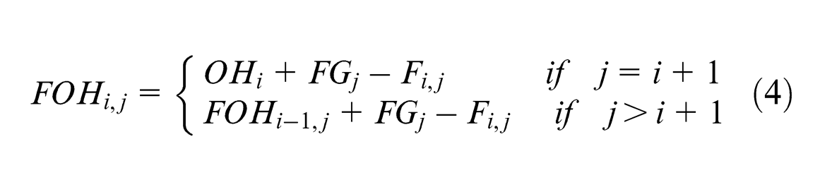
If the inventory level does not reach the timing of raising or lowering, calculate the expected inventory after one lead time according to market forecast information, which is viewing market forecast information as actual customer demand. Set FOH_{i, j} and calculate jth period of expected inventory at ith period; FOH_{i, j} is calculated as

F O H_{i, j} = {\begin{array}{l} O H_{i} + F G_{j} - F_{i, j} & i f & j = i + 1 \\ F O H_{i - 1, j} + F G_{j} - F_{i, j} & i f & j > i + 1 \end{array}

(4)

After calculating expected inventory, raise or lower inventory according to the expected inventory. The policies of adjusting replenishment by the expected inventory are as follows:

1. When inventory level is in the yellow zone and expected inventory is out of stock, raise replenishment quantity.

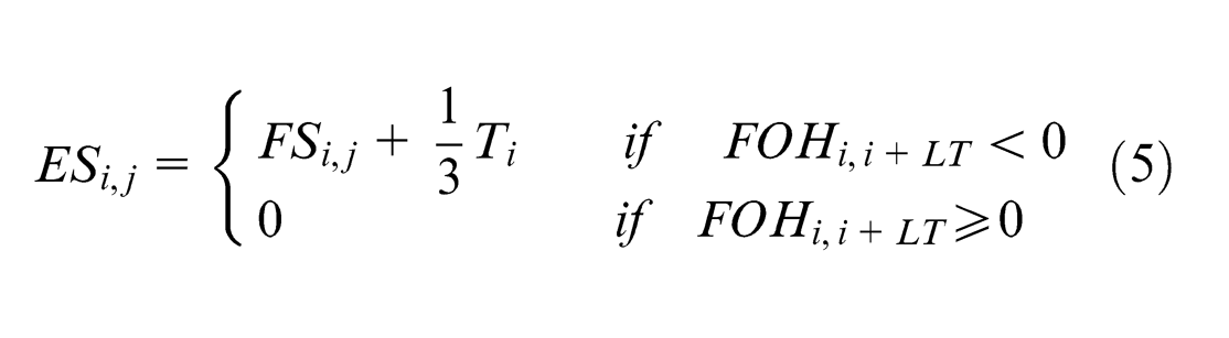
If expected inventory after one lead time is minus, it indicates that out of stock may happen in the future; then raise replenishment quantity as “current actual demand + forecast volume of out of stock + one-third of inventory buffer” for raising expected inventory to yellow zone. Assume ES_{i, j} expresses increased replenishment quantity for jth period at ith period. Therefore, ES_{i, j} can be represented as

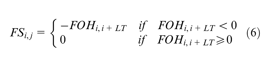
E S_{i, j} = {\begin{array}{l} F S_{i, j} + \frac{1}{3} T_{i} & i f & F O H_{i, i + L T} < 0 \\ 0 & i f & F O H_{i, i + L T} \geq 0 \end{array}

(5)

FS_{i, j} represents forecast volume of out of stock for jth period at ith period, expressed as

F S_{i, j} = {\begin{array}{l} - F O H_{i, i + L T} & i f & F O H_{i, i + L T} < 0 \\ 0 & i f & F O H_{i, i + L T} \geq 0 \end{array}

(6)

Assume TES_k is total adjustment replenishment quantity, which expresses sum of increase or decrease of replenishment quantity, and TES_k represents

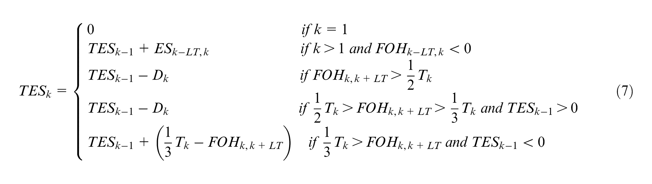
T E S_{k} = {\begin{array}{l} 0 & i f k = 1 \\ T E S_{k - 1} + E S_{k - L T, k} & i f k > 1 a n d F O H_{k - L T, k} < 0 \\ T E S_{k - 1} - D_{k} & i f F O H_{k, k + L T} > \frac{1}{2} T_{k} \\ T E S_{k - 1} - D_{k} & i f \frac{1}{2} T_{k} > F O H_{k, k + L T} > \frac{1}{3} T_{k} a n d T E S_{k - 1} > 0 \\ T E S_{k - 1} + (\frac{1}{3} T_{k} - F O H_{k, k + L T}) & i f \frac{1}{3} T_{k} > F O H_{k, k + L T} a n d T E S_{k - 1} < 0 \end{array}

(7)

2. When inventory level is in the yellow zone and calculated expected inventory is more than half of the inventory buffer, lower replenishment quantity.

3. When inventory level is in the yellow zone and calculated expected inventory is between one-third and half of the inventory buffer, and total adjustment replenishment quantity (TES_k_{- 1}) at the preceding period is greater than 0, lower replenishment quantity. On the other hand, if total adjustment replenishment quantity (TES_k_{- 1}) at the preceding period is less than or equal to 0, the current replenishment is in accordance with the actual customer demand replenishment.

4. When inventory level is in the yellow zone and calculated expected inventory is located in the red zone, total adjustment replenishment quantity (TES_k_{- 1}) at the preceding period is less than 0; raise replenishment quantity.

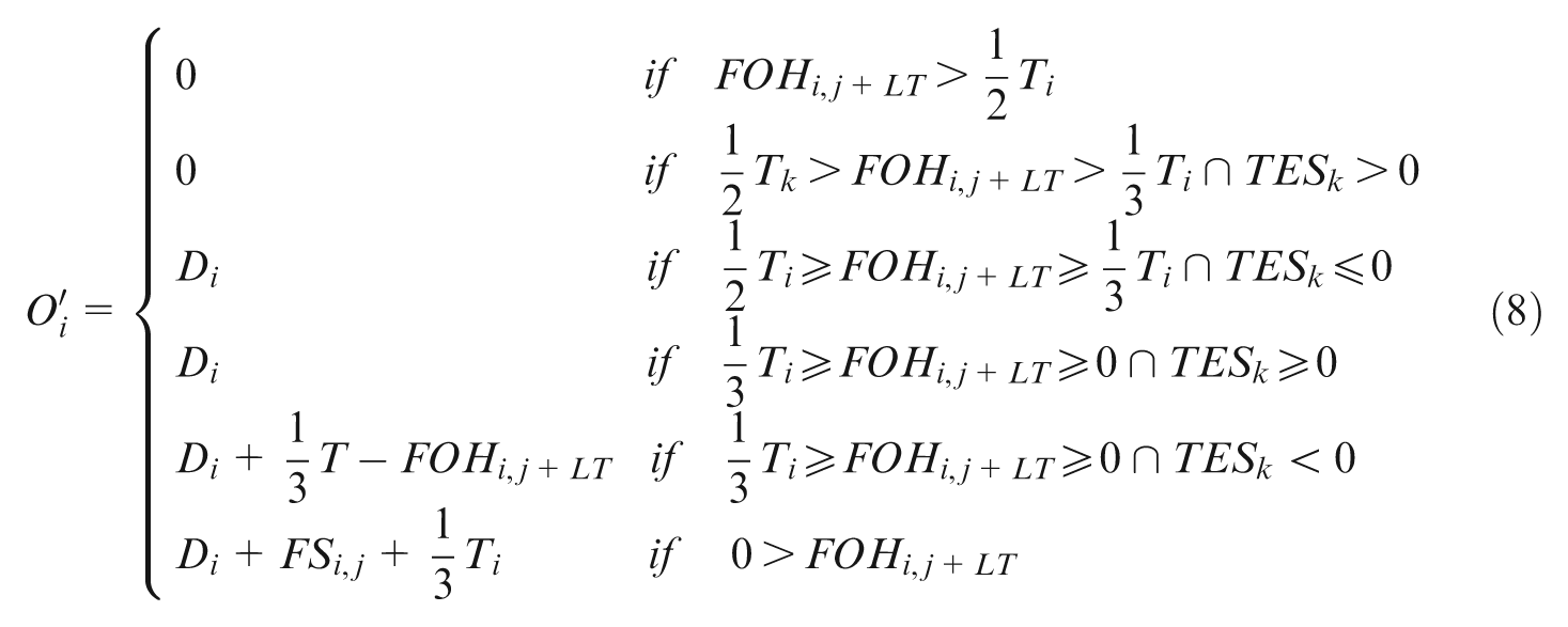
When inventory level is in yellow zone and forecast inventory is higher than one-second of inventory buffer, then lower replenishment, and volume of lowering equals current customer demand. That is, if forecast inventory after one lead time is higher than one-second of inventory buffer, the current replenishment is 0 and utilize equations (3) to (7) to count lowering volume into total revised replenishment.

This phenomenon indicates that lower replenishment quantity may cause out of stock in the future, so raise replenishment quantity; the additional volume is 1/3T_k−FOH_{k, k+LT} and then calculate TES_k by equation (4). If expected inventory is located in the red zone but total adjustment replenishment quantity (TES_k) is greater than or equal to 0, the current replenishment is in accordance with the actual customer demand replenishment.

Therefore, adjusted replenishment quantity by market forecast information ${O^{'}}_{i}$ is expressed as follows

{O^{'}}_{i} = {\begin{array}{l} 0 & i f F O H_{i, j + L T} > \frac{1}{2} T_{i} \\ 0 & i f \frac{1}{2} T_{k} > F O H_{i, j + L T} > \frac{1}{3} T_{i} \cap T E S_{k} > 0 \\ D_{i} & i f \frac{1}{2} T_{i} \geq F O H_{i, j + L T} \geq \frac{1}{3} T_{i} \cap T E S_{k} \leq 0 \\ D_{i} & i f \frac{1}{3} T_{i} \geq F O H_{i, j + L T} \geq 0 \cap T E S_{k} \geq 0 \\ D_{i} + \frac{1}{3} T - F O H_{i, j + L T} & i f \frac{1}{3} T_{i} \geq F O H_{i, j + L T} \geq 0 \cap T E S_{k} < 0 \\ D_{i} + F S_{i, j} + \frac{1}{3} T_{i} & i f 0 > F O H_{i, j + L T} \end{array}

(8)

Procedure of the proposed approach

The flow chart of integrating market demand forecast and demand-pull replenishment is shown in Figure 3; the procedure of the proposed approach is as follows:

Step 1. Calculate inventory level by equation (2).

Step 2. According to the inventory level (OH_i), decide whether to adjust inventory buffer (T_i).

1. If inventory level is in the red zone continuously for r period, raise the inventory buffer. The replenishment quantity is set to O_i = D_i+T_i×IT in the current period. Then go to step 4.

2. If inventory level is in the green zone continuously for g period, lower the inventory buffer. Then go to step 4.

3. If inventory level is in the yellow zone, the inventory buffer does not need to adjust. Then go to step 3.

Step 3. Calculate expected inventory FOH_{i, i+LT} by equation (4) according to market forecast information to decide whether to adjust replenishment quantity.

1. If FOH_{i, i+LT} is lower than 0, then the replenishment quantity is set to O_i = D_i+FS_{i, j}+ 1/3T_i in the current period.

2. If FOH_{i, i+LT} is larger than 1/2 T_i, then the replenishment quantity is set to O_i = 0 in the current period. Calculate the total adjustment replenishment quantity (TES_i) in the current period by equation (7).

3. If FOH_{i, i+LT} is between 1/2 T_i and 1/3 T_i and total adjustment replenishment quantity in the preceding period (TES_i_-1) is larger than 0, then the replenishment quantity is set to O_i = 0 in the current period. Calculate the total adjustment replenishment quantity (TES_i) in the current period by equation (7).

4. If FOH_{i, i+LT} is between 1/2 T_i and 1/3 T_i and total adjustment replenishment quantity in the preceding period (TES_{i -}₁) is less than or equal to 0, then the replenishment quantity is set to O_i = D_i. Calculate the total adjustment replenishment quantity (TES_i) in the current period by equation (7).

5. If FOH_{i, i+LT} is in the red zone and total adjustment replenishment quantity in the preceding period (TES_{i -}₁) is greater than or equal to 0, then the replenishment quantity is set to O_i = D_i.

6. If FOH_{i, i+LT} is in the red zone and total adjustment replenishment quantity in the preceding period (TES_{i -}₁) is less than 0, then the replenishment quantity is set to O_i = D_i+ (1/3 ×T_i−FOH_{i, i+LT}) in the current period.

Step 4. Send out replenishment needs.

Figure 3.

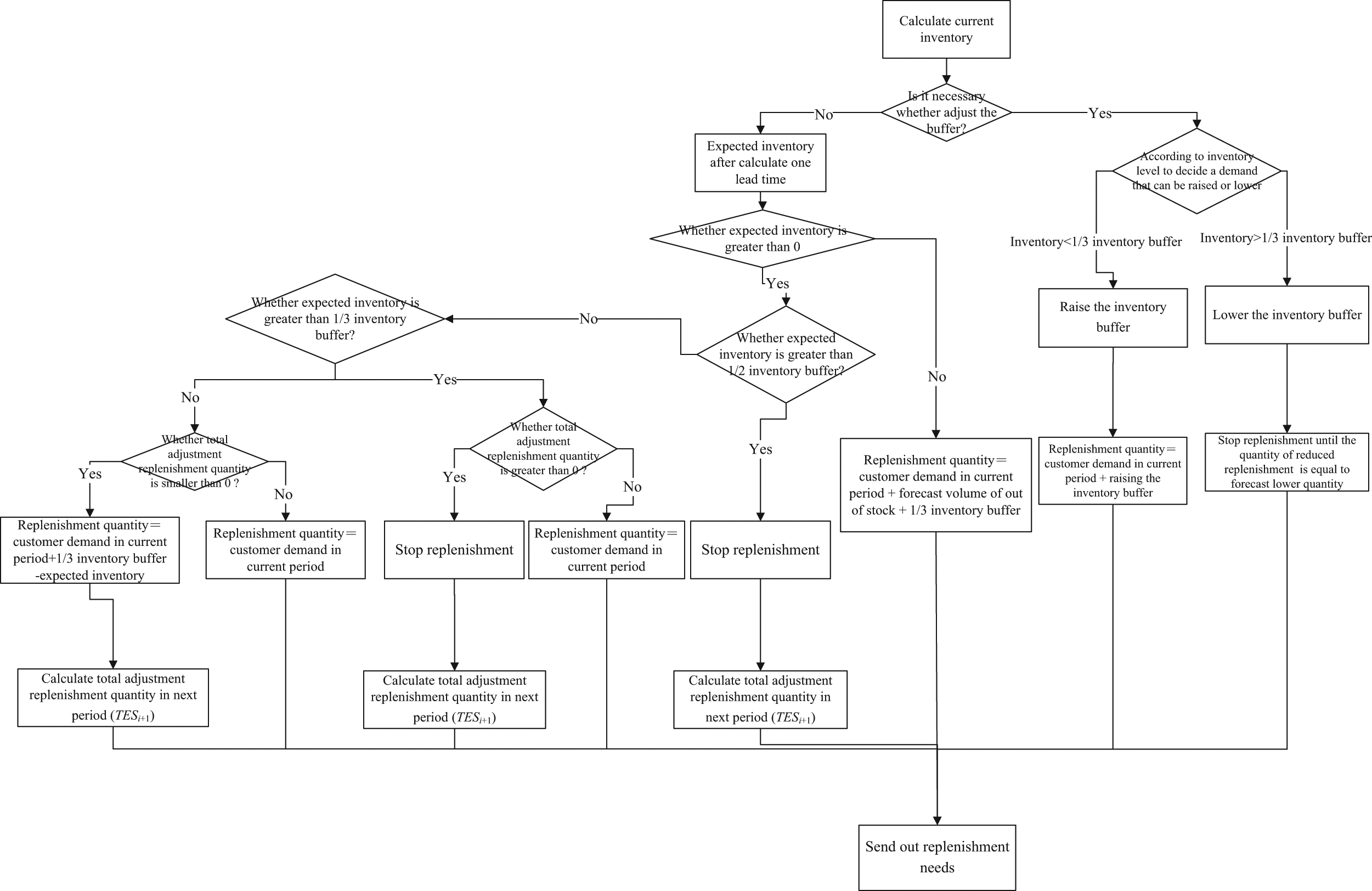
Flow chart to determine per period replenishment.

Related performance measurement indicators

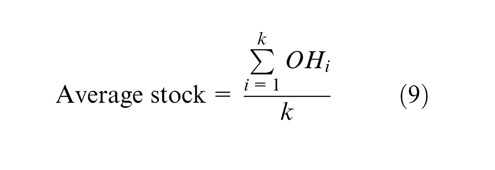
Average stock

It represents average stock in a warehouse every period, calculated as

Average stock = \frac{\sum_{i = 1}^{k} O H_{i}}{k}

(9)

Service level

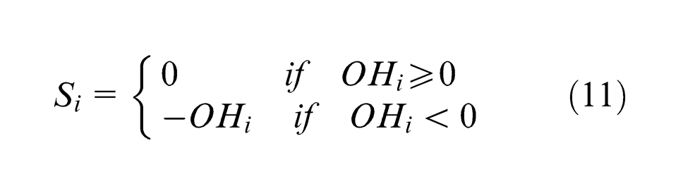
It represents the level of satisfied demand for assessing the out of stock, calculated as

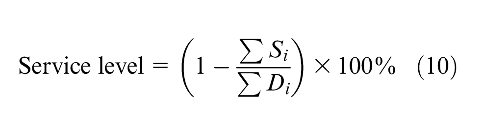
Service level = (1 - \frac{\sum S_{i}}{\sum D_{i}}) \times 100 %

(10)

where S_i represents the out of stock per period when inventory level cannot satisfy demand, calculated as

S_{i} = {\begin{array}{l} 0 & i f & O H_{i} \geq 0 \\ - O H_{i} & i f & O H_{i} < 0 \end{array}

(11)

Case study

In this section, this article uses a real case of a wafer product that was drawn from a professional wafer foundry company (A Company), which is well known for wafer foundry in Taiwan, to demonstrate the proposed approach. This article compares differences of average stock and service levels between demand-pull with market forecast information and original demand-pull policy.

Overview

The data are supplied from A company, which contain the product demand information with customer forecast from October 2009 to April 2010 (27 weeks). Related properties of this product are as follows

Replenishment lead time is 9 weeks.

The replenishment cycle is 1 week.

Allow backorder.

The factory does not allow crashing.

Assume initial inventory buffer is within the lead time of replenishment, which is the product of the maximum amount of the forecast demand provided by the customer (weeks 1–9 in this case) and replenishment lead time.

The initial preheating time is 9 weeks for the warehouse having sufficient time to construct initial inventory buffer.

The setting parameters of demand-pull are assumed such that the red zone reactor (r) is 1 and green zone reactor (g) is 1, and both the enlarge proportion and reduce proportion are 0.33.

Data analysis

This article analyzes 27 weeks of real product demand supplied by A company and weekly market forecast information provided by customers of A company. The product average demand is 1064, and standard error is 567.82. Mean absolute percentage error (MAPE) of market forecast information is 31.95%. Through analysis and calculation, average stock of unused market forecast information is 2282 and service level is only 82.91%, but average stock of used market forecast information rises to 5531 and service level increases to 99.86%. The comparative diagram for inventory in the simulated case is shown in Figure 4. This diagram indicates that integrating market demand forecast information and demand-pull replenishment can avoid being out of stock after 15 weeks by keeping enough inventories.

Figure 4.

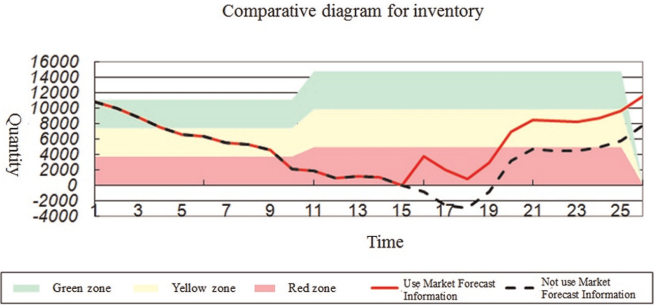
Comparative diagram for inventory in simulated case.

Simulation of the demand pattern

Simulation of the demand

General product demand pattern is divided into no trend or seasonality, only seasonal fluctuation, seasonal fluctuation and a positive trend, seasonal fluctuation and a negative trend, and mix trend. Zhao et al.²⁷ proposed a demand model, as shown in equation (12)

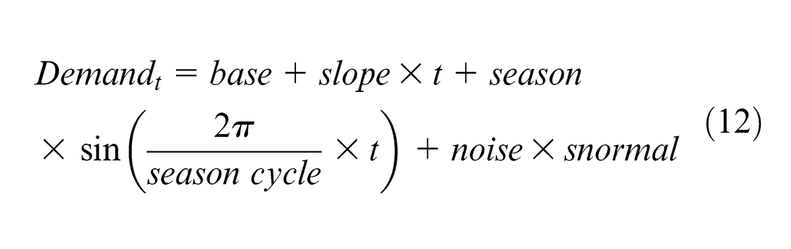
\begin{array}{l} D e m a n d_{t} = b a s e + s l o p e \times t + s e a s o n \\ \times \sin (\frac{2 π}{s e a s o n c y c l e} \times t) + n o i s e \times s n o r m a l \end{array}

(12)

The base is base quantity demanded; slope expresses demand index for long-term upward or downward trend; season indicates volatility of the seasonal cycle; season cycle is the time of season cycles, which is the number of periods between two demand peaks; noise means the degree of variation of short-term demand; and snormal is a standard normal random number, which is between -3.0 and +3.0.

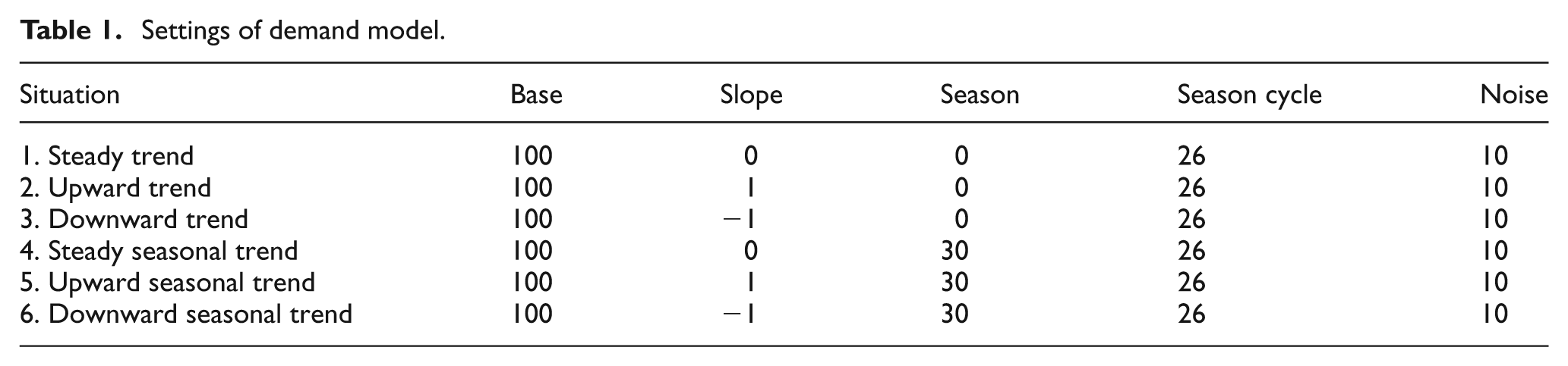
This article used equation (12) to generate randomized demand, and simulated time t is 104 periods. Table 1 represents settings of the demand model, and Figure 5 represents simulated demands generated from Table 1. This article probed six different trends of demand patterns: steady trend, upward trend, downward trend, steady seasonal trend, upward seasonal trend, and downward seasonal trend and used short-term fluctuations (noise) to control the size of the demand variability.

Table 1.

Settings of demand model.

Situation	Base	Slope	Season	Season cycle	Noise
1. Steady trend	100	0	0	26	10
2. Upward trend	100	1	0	26	10
3. Downward trend	100	−1	0	26	10
4. Steady seasonal trend	100	0	30	26	10
5. Upward seasonal trend	100	1	30	26	10
6. Downward seasonal trend	100	−1	30	26	10

Figure 5.

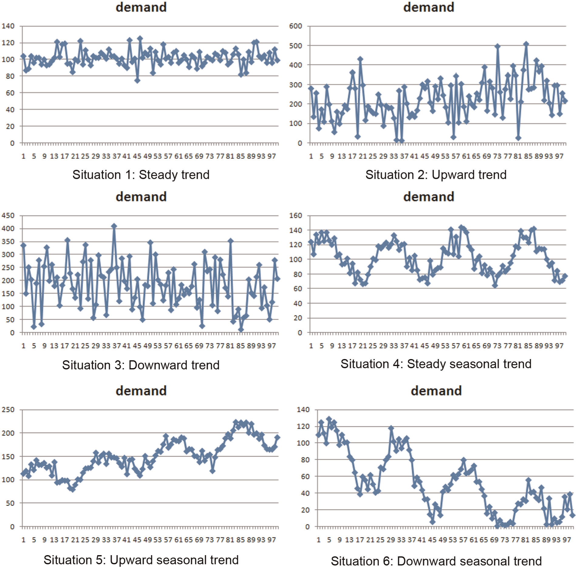
Line chart of simulated demand.

Market forecast information

This article used the rolling forecast as a reference for replenishment planning per period. Because longer forecast time causes lower forecast accuracy, this article only takes replenishment lead time of forecast information as the basis for calculating expected inventory. Assuming that the bias follows a normal distribution and considering being farther away from the actual demand values will cause a greater variation of the predictive value. Therefore, this article used distance actual demand days and replenishment lead time proportion as the weights. The formula of forecast information can be expressed as shown in equation (13)

F_{i, j} = D_{j} \pm \frac{j - i}{L T} \times N (μ, σ)

(13)

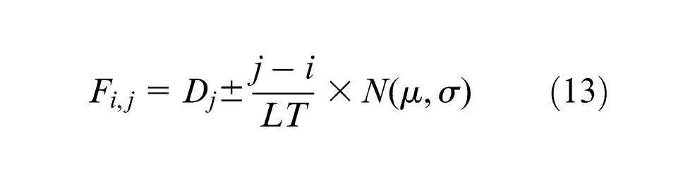
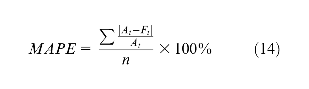
F_{i, j} expresses forecast jth period at ith period. Because the bias is influenced by the distance actual demand days, longer forecast days caused greater differences between forecast values and actual values. For example, assume replenishment lead time is 9 weeks; then, the predictive value of week 10 at week 1 is $F_{1, 10} = D_{10} \pm ((10 - 1) / 9) \times N (μ, σ)$ , and the predictive value of week 10 at week 5 is $F_{5, 10} = D_{10} \pm ((10 - 5) / 9) \times N (μ, σ)$ .

The MAPE is used to measure the accuracy of the forecast demands from the actual demands and is defined by equation (14). A_t represents actual value and F_t is the forecast value in period t

M A P E = \frac{\sum \frac{| A_{t} - F_{t} |}{A_{t}}}{n} \times 100 %

(14)

Due to the rolling forecast to update the predictive value per period, this article applied planning replenishment quantity to see predictive value and the distance from the actual demand replenishment lead time before the predictive value as the basis for calculating. The formula of MAPE can be expressed as shown in equation (15)

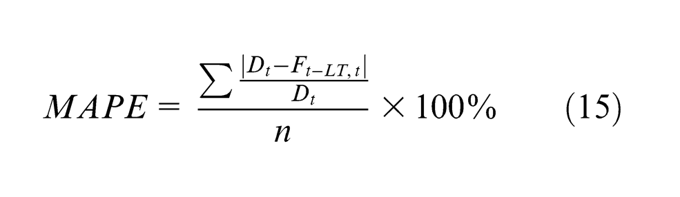
M A P E = \frac{\sum \frac{| D_{t} - F_{t - L T, t} |}{D_{t}}}{n} \times 100 %

(15)

D_t expresses actual demand at t period, and F_t−LT,t expresses predictive value of t period at t−LT period. For example, Table 2 is an instance of rolling forecast. Row 2 in this table represents predictive values of week 10 at every week, and predictive value of week 10 at week 10 indicates actual demand at week 11.

Table 2.

Example of rolling forecast.

Week	1	2	3	4	5	6	7	8	9	10	11	12
⋮	⋮	⋮	⋮	⋮	⋮	⋮	⋮	⋮	⋮	⋮	⋮	⋮
10	734	842	48	572	302	95	485	453	462	451
11		2409	1818	1712	1249	1275	1008	799	851	789	820
12			2758	2793	3117	3063	2710	2583	2062	1845	1728	1747

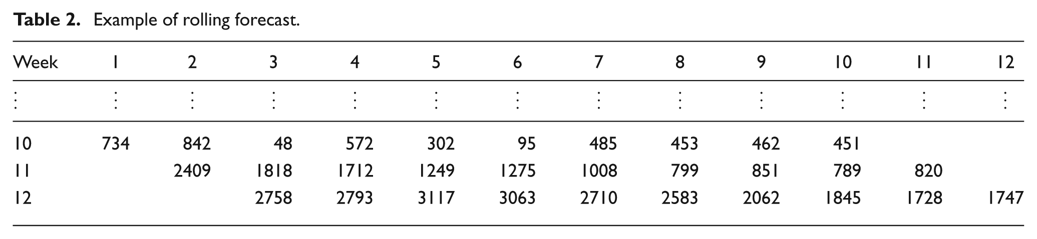
MAPE value can be calculated by the predictive value and the actual demand from Table 2

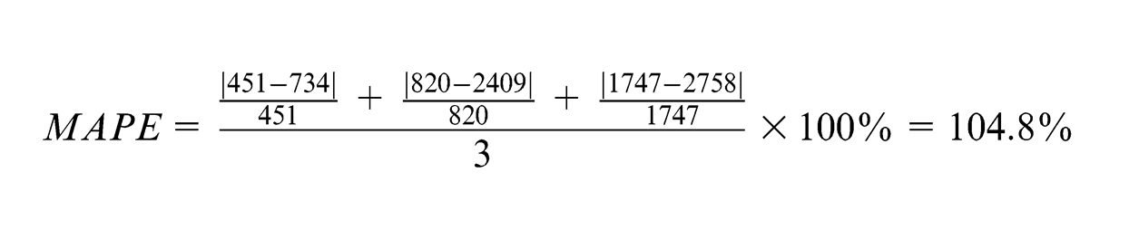
M A P E = \frac{\frac{| 451 - 734 |}{451} + \frac{| 820 - 2409 |}{820} + \frac{| 1747 - 2758 |}{1747}}{3} \times 100 % = 104.8 %

It represents that the predictive value is higher than the actual demand by an average of 104.8%.

Simulated data analysis

Numerical results are determined by the assumptions concerning the model parameters.²⁸ Therefore, this article used different MAPEs (sensitivity analysis) to compare average stock and service level.

Situation 1: steady trend

Figure 6(a) represents demand and the forecast line chart under the steady trend generated by equation (12). The solid line in this figure is the actual demand line chart, demand base value base is 100, the noise of short-term demand variation is set to 10, average demand is 109.74, and standard variation is 50.81. The dotted line is the market forecast demand line chart, and MAPE of market forecast information is 100%. In such a demand and forecast accuracy, average stock for using market forecast information is 896 and service level is 100%; average stock for not using market forecast information is 943 and service level is 100%. The average stock for not using market forecast information is higher than using market forecast information. Figure 6(b) is a comparison diagram for demand-pull replenishment using and not using market forecast information of a steady trend. The dotted line is an inventory line chart of not using market forecast information, and the solid line is an inventory line chart of using market forecast information. In this figure, the demand-pull replenishment can control inventory in the yellow zone effectively in the steady demand, to avoid excessively high or low amounts of inventory. Using market forecast information can reflect market demand more rapidly, and it only requires lower inventory than when not using market forecast information.

Figure 6.

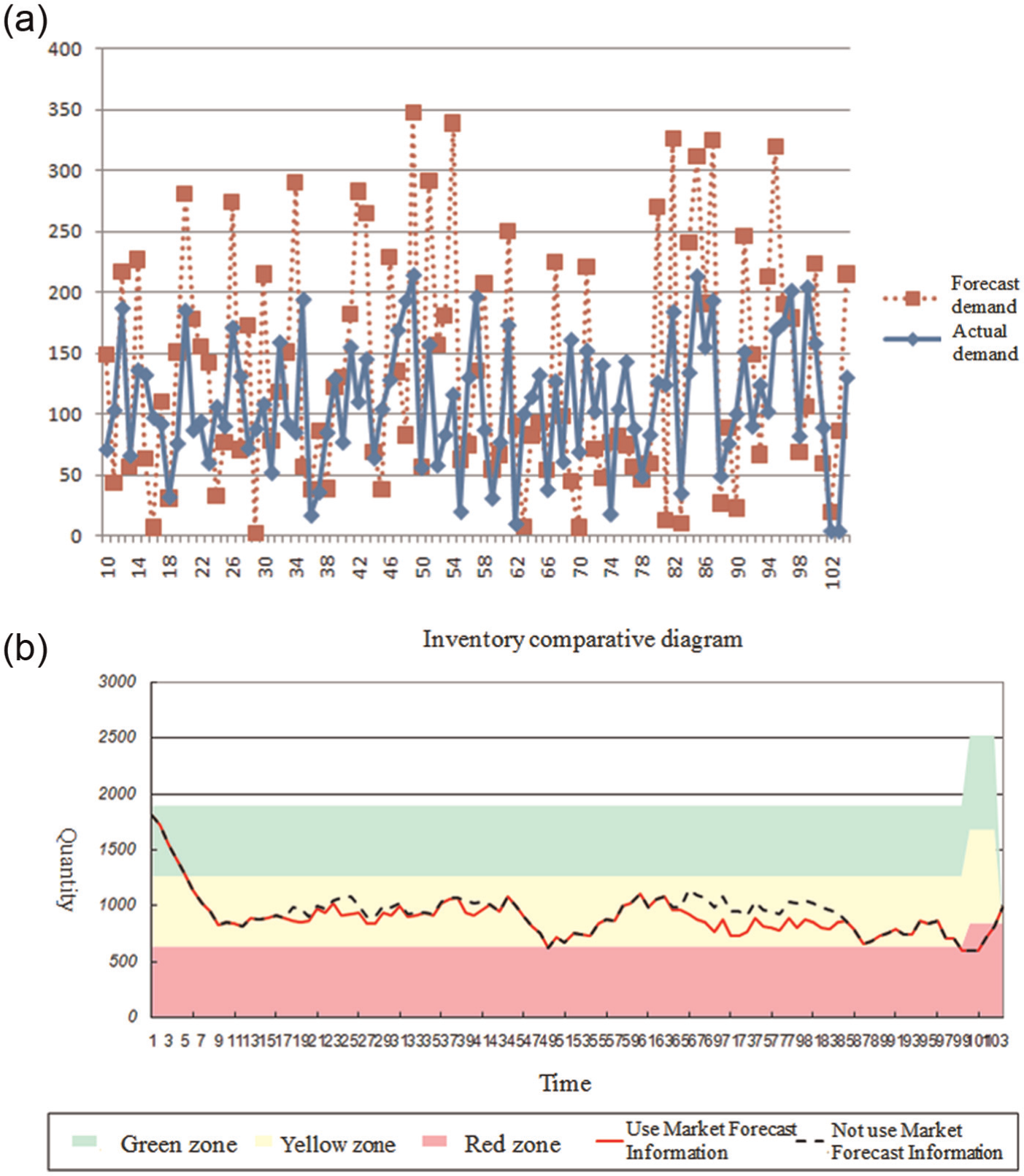
(a) Forecast line chart and (b) inventory comparison of the steady trend.

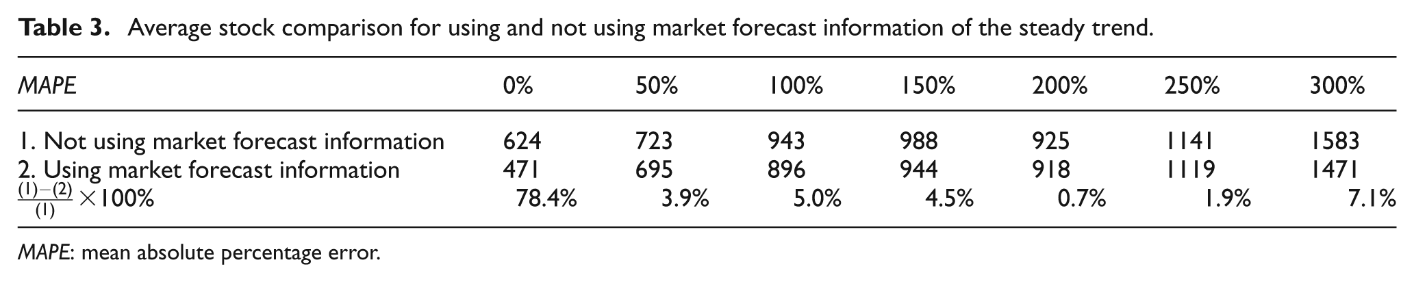
Table 3 is an average stock comparison table for using market forecast information and not using market forecast information in different forecast accuracies. The service levels of using market forecast information and not using market forecast information are both 100%. Besides, initial inventory buffer amount is established based on forecast information of period 1. From Table 3, we can see that using market forecast information can keep lower average stock in different forecast accuracies.

Table 3.

Average stock comparison for using and not using market forecast information of the steady trend.

MAPE	0%	50%	100%	150%	200%	250%	300%
1. Not using market forecast information	624	723	943	988	925	1141	1583
2. Using market forecast information	471	695	896	944	918	1119	1471
$\frac{(1) - (2)}{(1)} \times 100 %$	78.4%	3.9%	5.0%	4.5%	0.7%	1.9%	7.1%

MAPE: mean absolute percentage error.

Situation 2: upward trend

Figure 7(a) represents demand and the forecast line chart under the upward trend generated by equation (12). The solid line in this figure is actual demand line chart; demand base value base is 100 and demand increased one unit per period with the time; the noise of short-term demand variation is set to 10; average demand is 227.83; and standard variation is 104.28. The dotted line is a market forecast demand line chart, and MAPE of market forecast information is 102%. In such a demand and forecast accuracy, average stock for using market forecast information is 1714; average stock for not using market forecast information is 1868, and both service levels equal 100%. Figure 7(b) is a comparison diagram for demand-pull replenishment using and not using market forecast information of an upward trend. In this figure, the demand-pull replenishment using forecast information almost keeps the same or lower inventory than when not using market forecast information in the upward trend.

Figure 7.

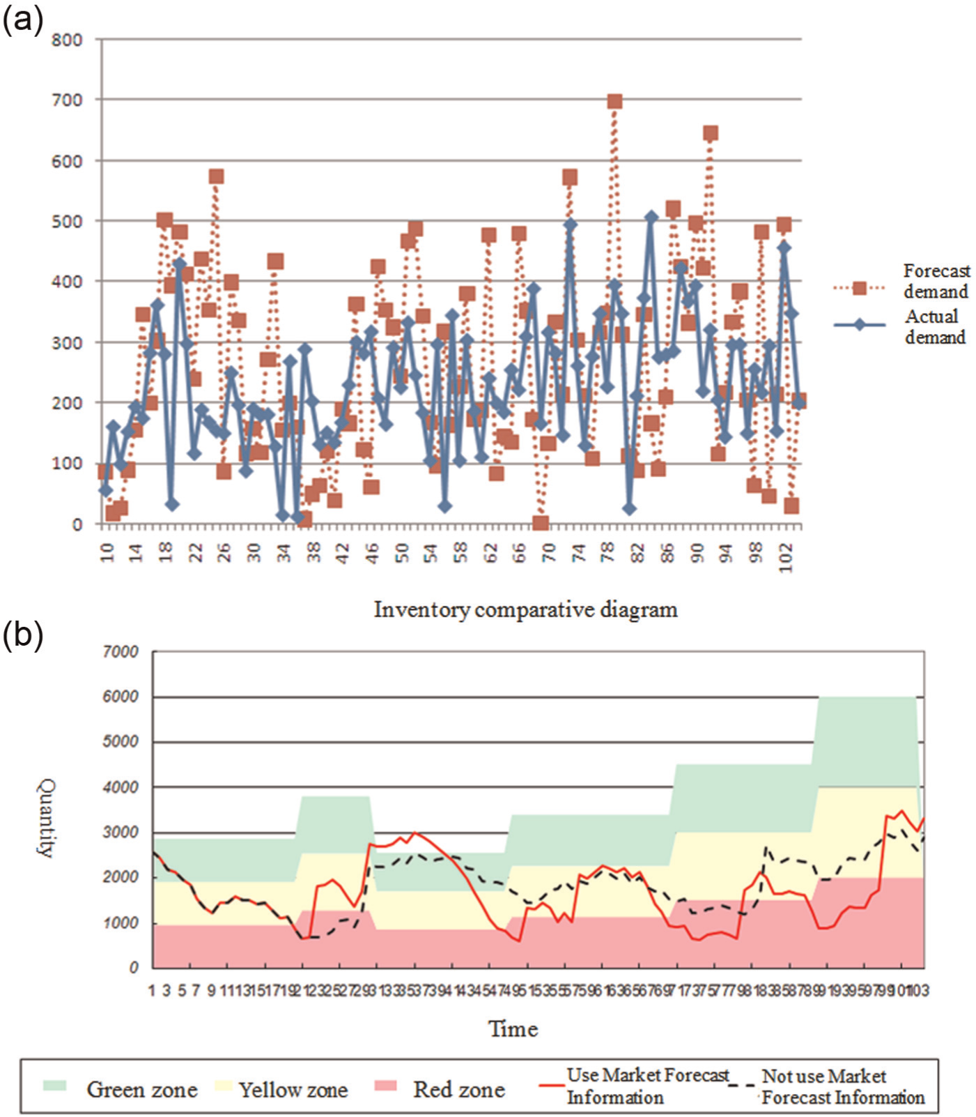
(a) Forecast line chart and (b) inventory comparison of the upward trend.

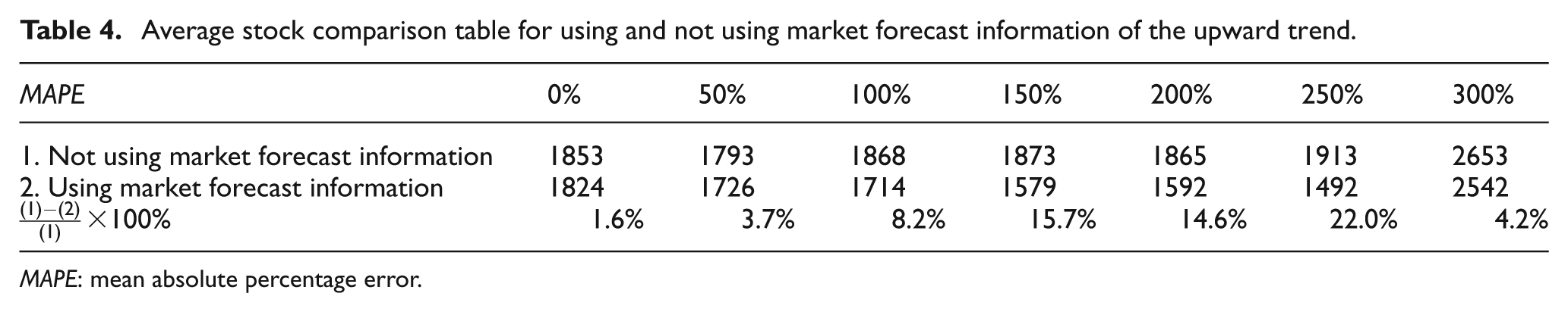
Average stock comparison table for using and not using market forecast information of the upward trend is shown in Table 4. The service levels of using and not using market forecast information are both 100%. From Table 4, we can see that using market forecast information can keep lower average stock in a different forecast accuracy.

Table 4.

Average stock comparison table for using and not using market forecast information of the upward trend.

MAPE	0%	50%	100%	150%	200%	250%	300%
1. Not using market forecast information	1853	1793	1868	1873	1865	1913	2653
2. Using market forecast information	1824	1726	1714	1579	1592	1492	2542
$\frac{(1) - (2)}{(1)} \times 100 %$	1.6%	3.7%	8.2%	15.7%	14.6%	22.0%	4.2%

MAPE: mean absolute percentage error.

Situation 3: downward trend

Figure 8(a) represents demand and the forecast line chart under the downward trend generated by equation (12). The solid line in this figure is the actual demand line chart; demand base value base is 100 and demand decreased one unit per period with the time; the noise of short-term demand variation is set to 10; average demand is 179.79; and standard variation is 87.2. The dotted line is a market forecast demand line chart, and MAPE of market forecast information is 100%. In such a demand and forecast accuracy, average stock for using market forecast information is 1944; average stock for not using market forecast information is 2262, and both service levels equal 100%. Figure 8(b) is a comparison diagram for demand-pull replenishment using and not using market forecast information of a downward trend. In this figure, the demand-pull replenishment of not using market forecast information causes slight increase of inventory because of decline in demand at the last period, and using market forecast information keeps lower inventory in the downward trend.

Figure 8.

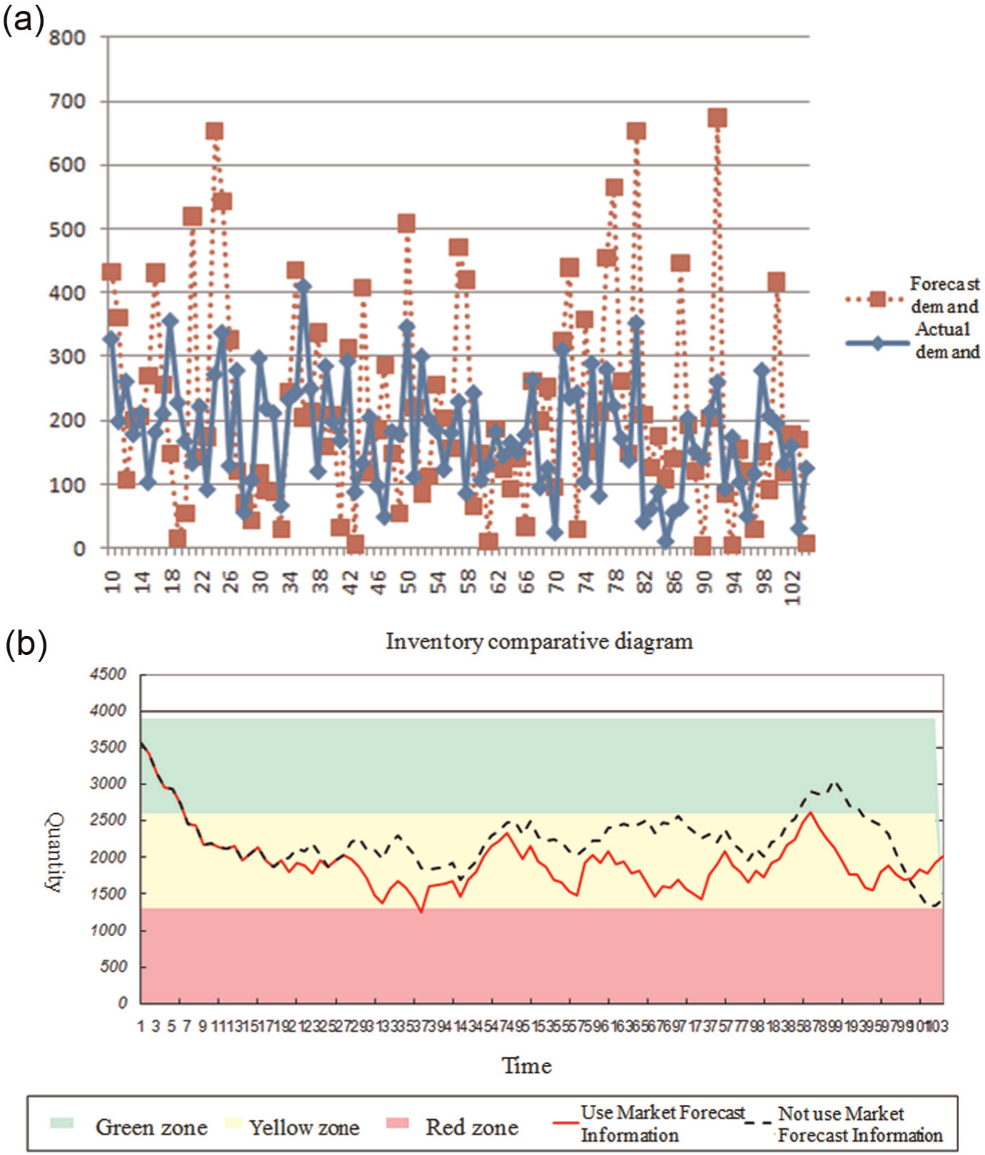
(a) Forecast line chart and (b) inventory comparison of the downward trend.

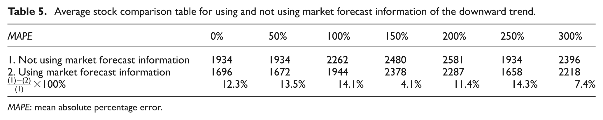
Table 5 is an average stock comparison table for using and not using market forecast information in a different forecast accuracy. The service levels of using and not using market forecast information are both 100%. From Table 5, we can see that using market forecast information can keep lower average stock in a different forecast accuracy and can reduce average stock about 10% in a larger forecast error.

Table 5.

Average stock comparison table for using and not using market forecast information of the downward trend.

MAPE	0%	50%	100%	150%	200%	250%	300%
1. Not using market forecast information	1934	1934	2262	2480	2581	1934	2396
2. Using market forecast information	1696	1672	1944	2378	2287	1658	2218
$\frac{(1) - (2)}{(1)} \times 100 %$	12.3%	13.5%	14.1%	4.1%	11.4%	14.3%	7.4%

MAPE: mean absolute percentage error.

Situation 4: steady seasonal trend

Figure 9(a) is the demand and the forecast line chart under the steady seasonal trend generated by equation (12). The solid line in this figure is actual demand line chart, demand base value base is 100, amplitude of the season cycle variable is 30, cycle time is 26 weeks, the noise of short-term demand variation is set to 10, average demand is 102.11, and standard variation is 21.74. The dotted line is market forecast demand line chart, and MAPE of market forecast information is 100%. In such a demand and forecast accuracy, average stock for using market forecast information is 1291; average stock for not using market forecast information is 1348, and both service levels equal 100%. Figure 9(b) is a comparison diagram for demand-pull replenishment using and not using market forecast information of the steady seasonal trend. In this figure, the demand-pull replenishment using forecast information reduces the demand quantity before reducing the inventory buffer and keeps inventory lower at the steady seasonal trend.

Figure 9.

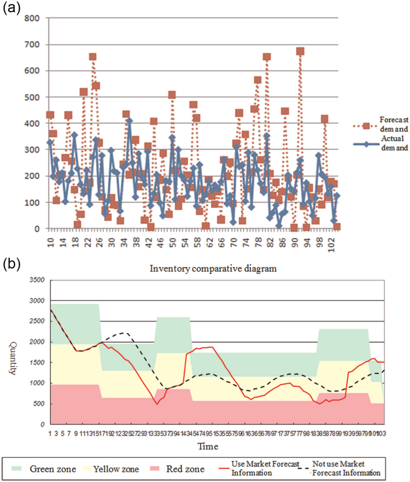
(a) Forecast line chart and (b) inventory comparison of the steady seasonal trend.

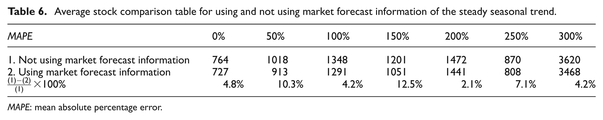
Average stock comparison table for using and not using market forecast information of the steady seasonal trend is shown in Table 6. The service levels of using and not using market forecast information are both 100%. From Table 6, we can see that using market forecast information can keep average stock lower in a different forecast accuracy.

Table 6.

Average stock comparison table for using and not using market forecast information of the steady seasonal trend.

MAPE	0%	50%	100%	150%	200%	250%	300%
1. Not using market forecast information	764	1018	1348	1201	1472	870	3620
2. Using market forecast information	727	913	1291	1051	1441	808	3468
$\frac{(1) - (2)}{(1)} \times 100 %$	4.8%	10.3%	4.2%	12.5%	2.1%	7.1%	4.2%

MAPE: mean absolute percentage error.

Situation 5: upward seasonal trend

Figure 10(a) is the demand and the forecast line chart under the upward seasonal trend. The solid line in this figure is the actual demand line chart, demand base value base is 100, and demand increases one unit per period with the time. Amplitude of the season cycle variable is 30, cycle time is 26 weeks, the noise of short-term demand variation is set to 10, average demand is 152.71, and standard variation is 35.17. The dotted line is the market forecast demand line chart, and MAPE of market forecast information is 103%. In such a demand and forecast accuracy, average stock for using market forecast information is 1816; average stock for not using market forecast information is 1904, and both service levels equal 100%. Figure 10(b) is a comparison diagram for demand-pull replenishment using and not using market forecast information of the upward seasonal trend. In this figure, the demand-pull replenishment using market forecast information can keep inventory similar or even slightly lower than original demand-pull replenishment policy.

Figure 10.

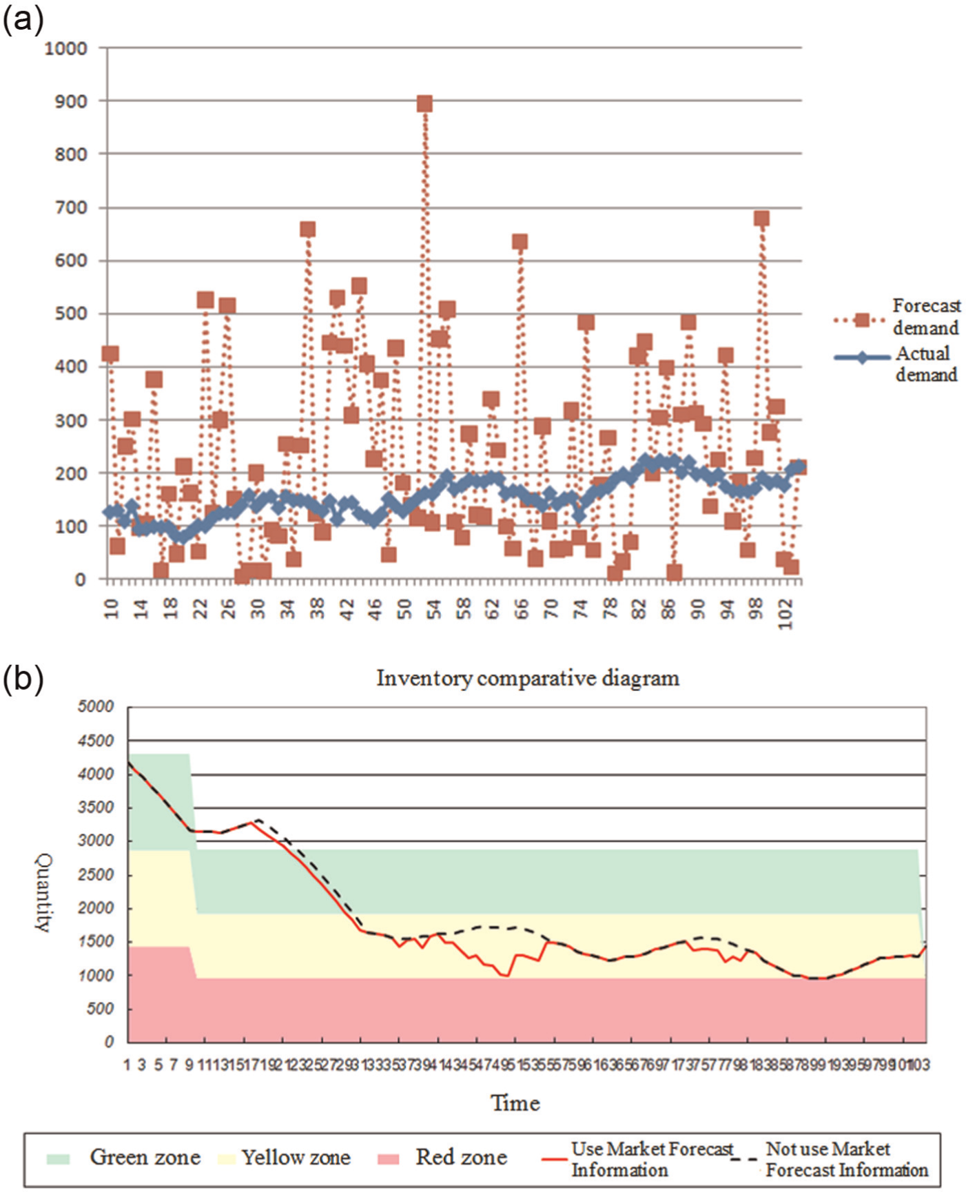
(a) Forecast line chart and (b) inventory comparison of the upward seasonal trend.

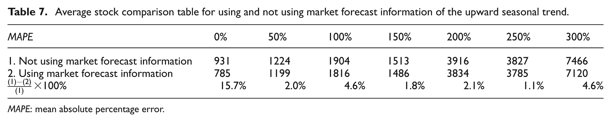
Table 7 is an average stock comparison table for using and not using market forecast information in a different forecast accuracy. The service levels of using and not using market forecast information are both 100%. From Table 7, we can see that using market forecast information can keep lower average stock in a different forecast accuracy.

Table 7.

Average stock comparison table for using and not using market forecast information of the upward seasonal trend.

MAPE	0%	50%	100%	150%	200%	250%	300%
1. Not using market forecast information	931	1224	1904	1513	3916	3827	7466
2. Using market forecast information	785	1199	1816	1486	3834	3785	7120
$\frac{(1) - (2)}{(1)} \times 100 %$	15.7%	2.0%	4.6%	1.8%	2.1%	1.1%	4.6%

MAPE: mean absolute percentage error.

Situation 6: downward seasonal trend

Figure 11(a) is the demand and the forecast line chart under the downward seasonal trend generated by equation (12). The solid line in this figure is the actual demand line chart, demand base value base is 100, and demand decreases one unit per period with time. Amplitude of the season cycle variable is 30, cycle time is 26 weeks, the noise of short-term demand variation is set to 10, average demand is 51.2, and standard variation is 35.3. The dotted line is the market forecast demand line chart, and MAPE of market forecast information is 100%. In such a demand and forecast accuracy, average stock for using market forecast information is 596; average stock for not using market forecast information is 647, and both service levels equal 100%. Figure 11(b) is a comparison diagram for demand-pull replenishment using and not using market forecast information of a downward seasonal trend. In this figure, the demand-pull replenishment using market forecast information reduces the demand quantity before reducing the inventory buffer and keeps inventory lower to an appropriate level.

Figure 11.

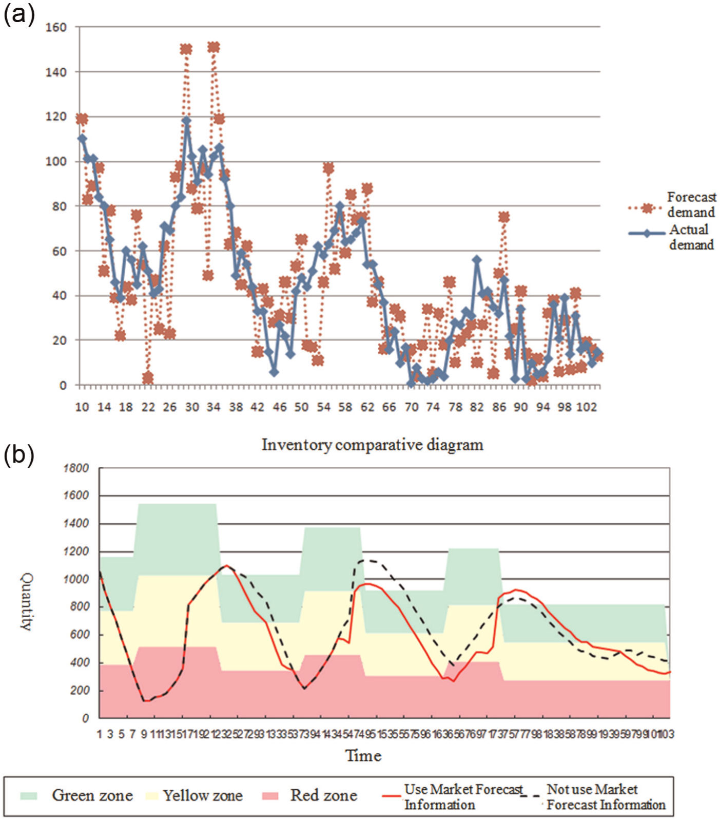
(a) Forecast line chart and (b) inventory comparison of the downward seasonal trend.

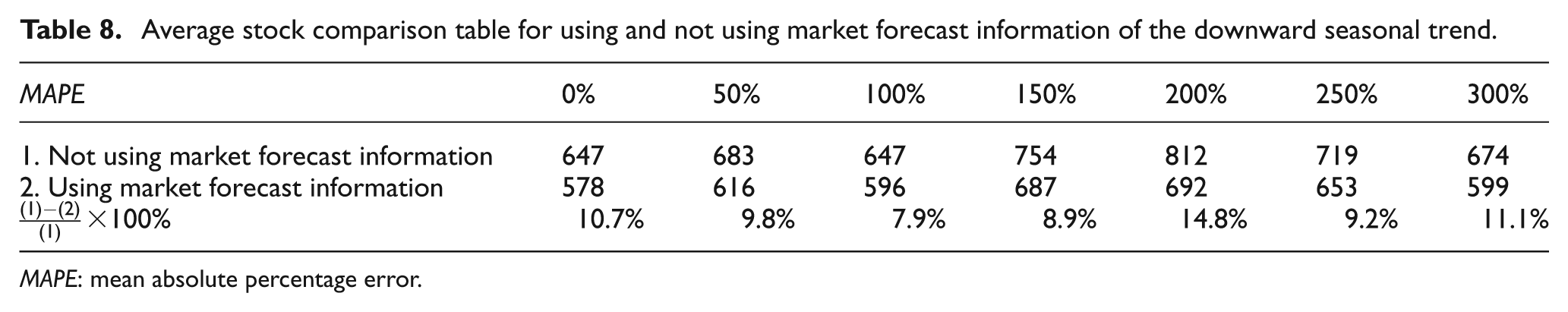
Average stock comparison table for using and not using market forecast information of the downward seasonal trend is shown in Table 8. The service levels of using and not using market forecast information are both 100%. From Table 8, we can see that using market forecast information can keep average stock lower in a different forecast accuracy.

Table 8.

Average stock comparison table for using and not using market forecast information of the downward seasonal trend.

MAPE	0%	50%	100%	150%	200%	250%	300%
1. Not using market forecast information	647	683	647	754	812	719	674
2. Using market forecast information	578	616	596	687	692	653	599
$\frac{(1) - (2)}{(1)} \times 100 %$	10.7%	9.8%	7.9%	8.9%	14.8%	9.2%	11.1%

MAPE: mean absolute percentage error.

Situation 7: product life cycle

This article divides demand into four stages: introduction stage, growth stage, maturity stage, and decline stage. The related settings are in Table 9.

Table 9.

Parameters setting of simulated product life cycle.

Demand periods	1–25	26–50	51–75	76–104
N(µ, σ)	N(100, 100)	N(500, 150)	N(900, 200)	N(750, 200)

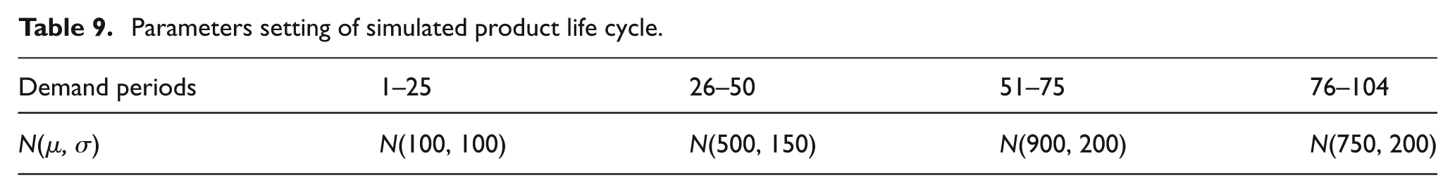
Figure 12(a) is the demand and the forecast line chart for considering product life cycle. The solid line in this figure is the actual demand line chart, average demand is 565.36, and standard variation is 354.78. The dotted line is the market forecast demand line chart, and MAPE of market forecast information is 101.83%. The results showed that the average stock for not using market forecast information is 968, and service level is 47.89%. The average stock for using market forecast information is 1481, and service level is 98.14%. It expresses that the demand-pull replenishment using market forecast information can deal with the demand of different stages than not using market forecast information. The inventory comparison diagram for considering product life cycle is shown in Figure 12(b).

Figure 12.

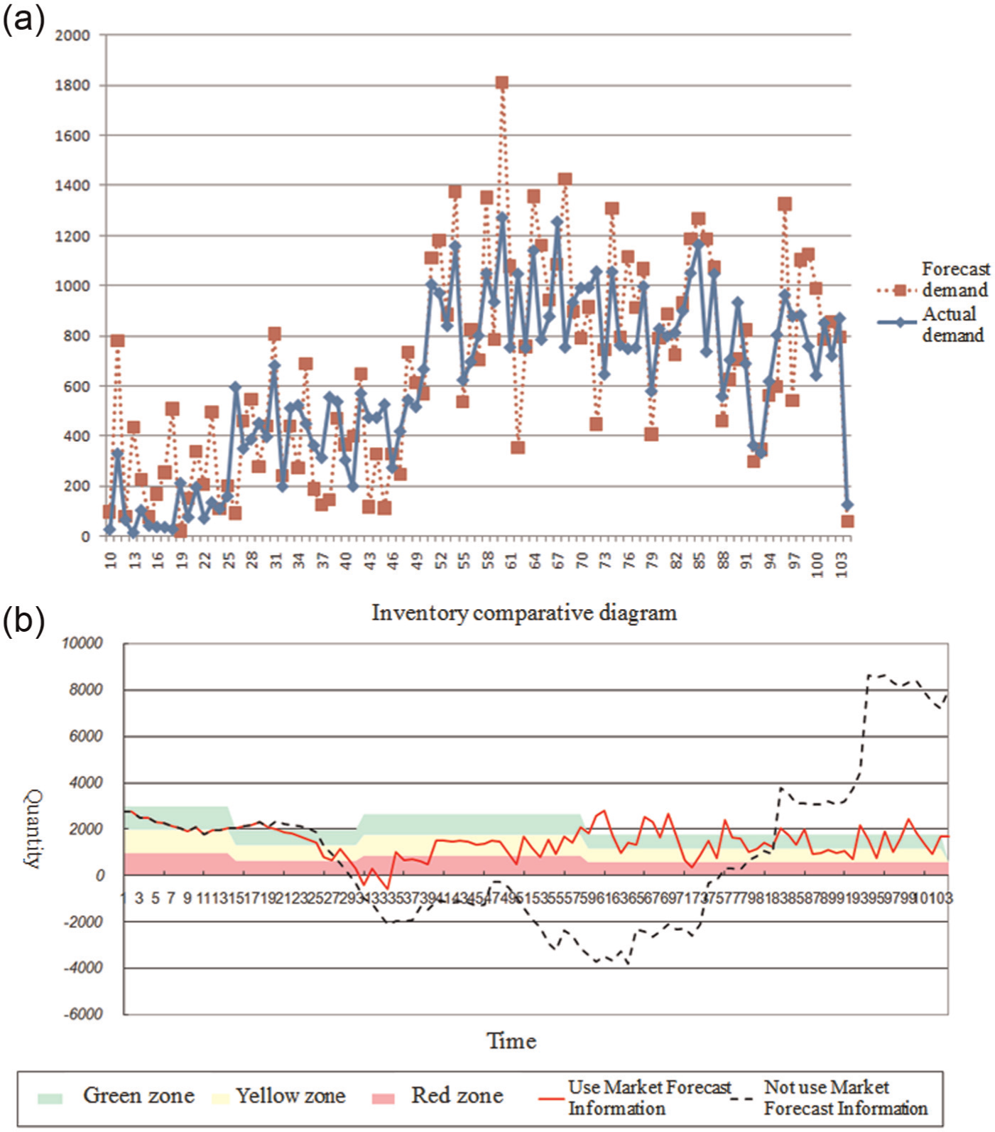
(a) Forecast line chart and (b) inventory comparison for considering product life cycle.

Average stock comparison table for using and not using market forecast information in a different forecast accuracy is shown in Table 10, and Table 11 represents the service level comparison table for using and not using market forecast information. These tables indicate that the average stock will gradually rise for using and not using market forecast information following a greater forecast error. Higher average stock can reach a higher service level of demand-pull replenishment for not using market forecast information but only rises to about 87.14%. Then, demand-pull replenishment for using market forecast information can reach above a 98% service level in any forecast accuracy. It indicates that demand-pull replenishment for using market forecast information can avoid being out of stock.

Table 10.

Average stock comparison table for considering product life cycle.

MAPE	0%	50%	100%	150%	200%	250%	300%
Not using market forecast information	1036	−157	968	232	3282	3681	4725
Using market forecast information	1132	1255	1481	1265	2962	3853	4136

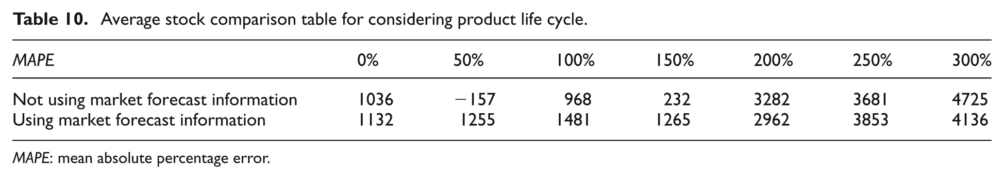
MAPE: mean absolute percentage error.

Table 11.

Service level comparison table for considering product life cycle.

MAPE	0%	50%	100%	150%	200%	250%	300%
Not using market forecast information	53.94%	36.73%	47.89%	38.99%	84.46%	86.07%	87.14%
Using market forecast information	100.00%	99.51%	98.14%	97.92%	100.00%	100.00%	98.71%

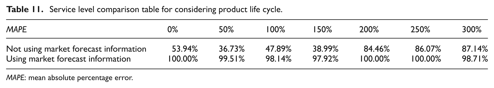
MAPE: mean absolute percentage error.

This section simulated and compared the demand-pull replenishment using and not using market forecast information according to different demand patterns. The results showed that the demand-pull replenishment can achieve a better service level and average stock in a more regular demand pattern, and using market forecast information can help the average stock reduce. Moreover, using market forecast information can help the demand-pull replenishment avoid being out of stock in a more irregular demand pattern. In a different forecast accuracy, the demand-pull replenishment using market forecast information can obtain a lower average stock than not using market forecast information.

Conclusion

TOC proposed combining buffer management and demand-pull replenishment to manage supply chain inventory; it is simple and easy to implement than in the past on practical applications. In the past studies, the traditional demand-pull replenishment approach appears to be out of stock in some larger demand variation situations. In order to solve this problem, this article proposes integrating market demand forecast information and demand-pull replenishment to improve the inventory management effectiveness for long lead times and large demand variations of wafer fabrication. The proposed approach can enlarge the application range of demand-pull replenishment to suit more demand patterns. Besides utilizing buffer management to adjust the buffer, it adjusts replenishment quantity according to market forecast information before not adjusting the amount of inventory buffer to advance in response to changes in demand. In a different forecast accuracy, the proposed approach is able to maintain higher service levels and lower average stock in some larger demand variation situations. Then, this article analyzes demand and forecast data supplied by the wafer manufacturing company and customers; the results found that the use of market forecast information can improve the service level and avoid being out of stock.

Besides the discussion of the actual case, this article used the findings by Zhao et al.,²⁷ who proposed a demand model and the influence of the product life cycle to generate simulated demand, according to different simulation requirements to perform a simulation analysis. After analyzing and comparing, the results show that using market forecast information of demand-pull replenishment can get a low average stock than when not using market forecast information of demand-pull replenishment. Furthermore, forecast accuracy will be a critical influence factor for using market forecast information of demand-pull replenishment.

Footnotes

Declaration of conflicting interests

The authors declare that there is no conflict of interest.

Funding

The authors gratefully acknowledge the funding provided by the National Science Council of the Republic of China under Contract Nos NSC 99-2410-H-009-049, NSC 101-2410-H-009-005-MY2, NSC 101-2410-H-145-001, and NSC 102-2410-H-145-001.

References

Goldratt

Cox

. The goal: a process of ongoing improvement. Croton-on-Hudson, NY: North River Press, 1984.

Chen

Tsai

. A study of an enhanced simulation model for TOC supply chain replenishment system under capacity constraint. Expert Syst Appl 2010; 37(9): 6435–6440.

Hung

Liou

Wen

. Decision support system for inventory management by TOC demand-pull approach. In: Proceedings of 2010 IEEE/SEMI advanced semiconductor manufacturing conference (ASMC 2010), San Francisco, CA, 11–13 July, pp. 23–26. New York: IEEE.

Tyan

Chen

Wang

. Development of a state-dependent dispatch rule using theory of constraints in near-real-world wafer fabrication. Prod Plan Control 2002; 13(3): 253–261.

Hsieh

Hou

. Production-flow-value-based job dispatching method for semiconductor manufacturing. Int J Adv Manuf Tech 2006; 30(7–8): 727–737.

Kuo

Chang

Huang

. Due-date performance improvement using TOC’s aggregated time buffer method at a wafer fabrication factory. Expert Syst Appl 2009; 36(2): 1783–1792.

Simatupang

Wright

Sridharan

. Applying the theory of constraints to supply chain collaboration. Supply Chain Manag 2004; 9(1): 57–70.

Watson

Blackstone

Gardiner

. The evolution of a management philosophy: the theory of constraints. J Oper Manag 2007; 25(2): 387–402.

Perry

Sohal

. Effective quick response practices in a supply chain partnership: an Australian case study. Int J Oper Prod Man 2001; 21(5–6): 840–854.

10.

Dellaert

Jeunet

. An alternative to safety stock policies for multi-level rolling schedule MRP problems. Eur J Oper Res 2005; 163(3): 751–768.

11.

Jeunet

. Demand forecast accuracy and performance of inventory policies under multi-level rolling schedule environments. Int J Prod Econ 2006; 103(1): 401–419.

12.

Archibald

Silver

. (s, S) policies under continuous review and discrete compound Poisson demand. Manage Sci 1978; 24(9): 899–909.

13.

Mak

Lai

. Analysis of optimal opportunistic replenishment policies for inventory systems by using a (s, S) model with a maximum issue quantity restriction. Eur J Oper Res 2005; 166(2): 385–405.

14.

Natarajan

Goyal

. Safety stocks in JIT environments. Int J Oper Prod Man 1994; 14(10): 64–71.

15.

Ehrhardt

. The power approximation for computing (s, S) inventory policies. Manage Sci 1979; 25(8): 777–786.

16.

Ehrhardt

Mosier

. A revision of the power approximation for computing (s, S) policies. Manage Sci 1984; 30(5): 618–622.

17.

Naddor

. Optimal and heuristic decisions in single and multi-item inventory systems. Manage Sci 1975; 21(11): 1234–1249.

18.

Babai

Syntetos

Teunter

. On the empirical performance of (T, s, S) heuristics. Eur J Oper Res 2010; 202(2): 466–472.

19.

Kim

. Coordinating an innovation in supply chain management. Eur J Oper Res 2000; 123(3): 568–584.

20.

Barbarosoglu

. An integrated supplier-buyer model for improving supply chain coordination. Prod Plan Control 2010; 11(8): 732–741.

21.

Kayis

Erhun

Plambeck

. Delegation vs control of component procurement under asymmetric cost information and simple contracts. Manuf Serv Oper Manag 2013; 15(1): 45–56.

22.

Zhang

Fine

. Dynamic business share allocation in a supply chain with competing suppliers. Oper Res 2013; 61(2): 280–297.

23.

Kurtulus

Ulku

Toktay

. The value of collaborative forecasting in supply chains. Manuf Serv Oper Manag 2012; 14(1): 82–98.

24.

Ozer

. Mechanism design for capacity planning under dynamic evolutions of asymmetric demand forecasts. Manage Sci 2013; 59(4): 987–1007.

25.

Chang

. TOC: Theory of constraints. Taipei, Taiwan: China Productivity Center, 2005.

26.

Fisher

Hammond

Obermeyer

. Making supply meet demand in an uncertain world. Harv Bus Rev 1994; 72(3): 83–93.

27.

Zhao

Xie

Lau

RSM

. Improving the supply chain performance: use of forecasting models versus early order commitments. Int J Prod Res 2001; 39(17): 3923–3939.

28.

Borgonovo

. Sensitivity analysis with finite changes: an application to modified EOQ models. Eur J Oper Res 2010; 200(1): 127–138.

Integrate market demand forecast and demand-pull replenishment to improve the inventory management effectiveness of wafer fabrication

Abstract

Keywords

Introduction

Literature review

Replenishment policy

(s, S) policy

(s, Q) policy

(R, S) policy

(R, s, S) policy

Supply chain coordination

TOC

Demand-pull replenishment

Buffer management

Throughput-dollar-days

Inventory-dollar-days

Methodology

Demand-pull replenishment

r: red zone reactor, r ∈ N

g: green zone reactor, g ∈ N

IT: enlarge proportion, IT ∈ R+

DT: reduce proportion, DT ∈ R+

Integrate market forecast information and demand-pull replenishment

Procedure of the proposed approach

Related performance measurement indicators

Average stock

Service level

Case study

Overview

Data analysis

Simulation of the demand pattern

Simulation of the demand

Market forecast information

Simulated data analysis

Situation 1: steady trend

Situation 2: upward trend

Situation 3: downward trend

Situation 4: steady seasonal trend

Situation 5: upward seasonal trend

Situation 6: downward seasonal trend

Situation 7: product life cycle

Conclusion

Footnotes

Declaration of conflicting interests

Funding

References