
Abstract
Demands for energy conservation and impact resistance have made high-strength steel a crucial material in sheet metal parts for the automotive industry. However, during metal stamping, the springback associated with high-strength steel plates is significantly greater than for mild steel. This makes numerical simulation and prediction in stamp forming extremely difficult. The Yoshida–Uemori material model comprehensively describes the Bauschinger effect and work hardening stagnation that occur in metal during cyclic large plastic deformation, making it an important model for the simulation of high-strength steel stamp forming. This study employed cyclic tension–compression tests and shear tests to explore the construction of a Yoshida–Uemori model and verify its accuracy using numerical simulation.
Introduction
As energy prices continue soaring, energy efficiency has become a basic requirement in modern automobiles. In addition, issues related to safety have made impact-resistant high-strength steel a material crucial to the automotive industry. However, the difficulties of forming high-strength steel often lead to splitting and springback and sidewall curl occur more frequently than with mild steel. Consequently, numerical simulation and prediction in the stamping of high-strength steel are extremely difficult.
The Yoshida–Uemori material model (YU model), proposed by Yoshida et al. 1 and Yoshida and Uemori, 2 combines the work hardening principles of isotropic hardening and kinematic hardening, enabling it to comprehensively describe the Bauschinger effect and work hardening that occur in metal during cyclic large plastic deformation. Thus, the YU model has been incorporated into several simulation software packages, such as the MAT_125 material model in LS-DYNA and the Yoshida kinematic hardening model in Pam-Stamp. In contrast, ABAQUS requires that users rewrite the custom material subroutines UMAT or VUMAT to define a YU model. In recent years, an increasing number of studies have applied the YU model to the simulation of metal stamping. For example, Hu et al. 3 employed LS-DYNA to analyze springback in automotive sheet metal parts, and Shi et al. 4 used LS-DYNA to simulate the stress–strain curve of high-strength steel in cyclic tension–compression tests in an investigation of YU material parameters. Ghaei et al. 5 and Ghaei and Green 6 developed an ABAQUS subroutine to establish a YU model and conducted a standard stamping experiment using NUMISHEET 2005 Benchmark 3, verifying that the YU model they developed could increase the accuracy of springback prediction.
There are a number of YU model parameters, many of which are obtained using curve fitting. Studies1,2 are rather vague in this respect, and as a result, many researchers have difficulty deriving these material parameters. Therefore, this study focused on the means to obtain the material parameters for YU models.
YU models are based on cyclic tension–compression tests. For sheet metal, buckling can occur easily during compression, thereby causing the experiment to fail. In Yoshida et al., 1 five specimens with a thickness of 1 mm were adhesively bonded together and a suitable fixture was selected for the cyclic tension–compression test. Researchers have also coordinated special fixtures using a single specimen to perform tension–compression tests. However, the measures adopted to prevent buckling come at the cost of limited strain and are thus inapplicable to deep drawing processes.
In cyclic shear tests, researchers can employ much higher levels of strain without fear of buckling. However, the use of YU models in shear tests has not been mentioned in previous studies. Thus, this study developed a methodology to convert the results of cyclic shear tests into those of equivalent tension–compression tests. Using the curve of the equivalent tension–compression test, we derived YU material parameters before applying LS-DYNA to construct a numerical model for cyclic shear tests. We then verified that YU material parameters can be used to simulate cyclic shear tests.
In incremental forming, Numerical Control (NC) machines serve as forming machines in which the cutting tool is replaced with a domed rod. The rod produces plastic deformation through the extrusion of the sheet metal, and the multiple increments of the forming procedure reduce the pressure requirements under the main axes. The extrusion effects of the rod constitute a single-point forming tool; therefore, extremely sophisticated forming results can be derived when coupled with complex die surfaces. For instance, Nguyen et al. 7 used a die in the shape of a human face and adopted incremental forming to reduce plastic deformation in the forming of an accurate facial mask of low-carbon steel. Using ABAQUS, they obtained results that were very close to those of the experiment. Because the pressure under the main axes of NC machines is limited, incremental forming is generally applied to softer materials, such as low-carbon steel, aluminum alloys, and titanium alloys, rather than high-strength steel. However, Babu and Kumar 8 succeeded in the incremental forming of AISI 304 steel with a thickness of 0.6 mm into a cone. The tensile strength of this material is close to that of high-strength steel; therefore, we believe that incremental forming will be applied to high-strength steel in the future. In such an event, the application scope of the YU model discussed in this study could be further extended to encompass incremental forming.
Conversion relationships between shear tests and equivalent tension–compression tests
Commonly used conversion relationships for tension experiments and shear experiments include the yield criteria of von Mises 9 and Hill’48. 10 We further included the yield criteria from Barlat’89 11 and Hill’90 12 to derive a conversion relationship between equivalent stress and equivalent strain.
von Mises yield criteria
The von Mises yield criterion is generally used for homogeneous and nonanisotropic materials; the formula for equivalent stress is
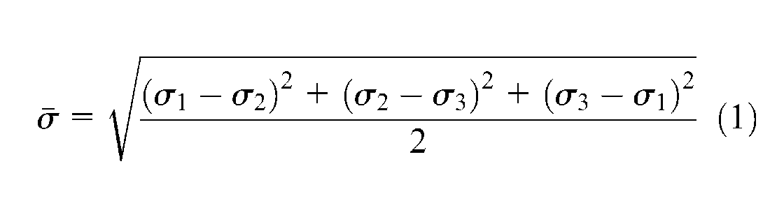
where
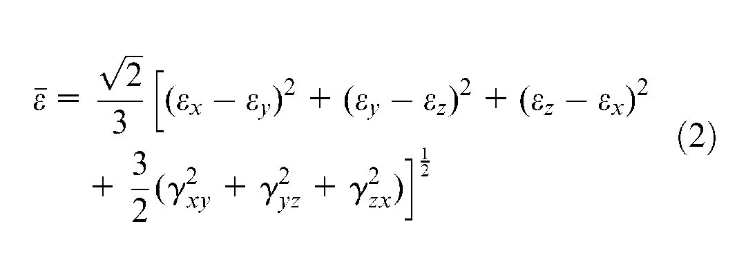
Figure 1 indicates the required yield stress values with the first principle stress and the secondary stress along various stress paths. Path 1, Path 2, Path 3, and Path 4 indicate the circumstances of uniaxial tension tests, plane-strain tensile tests, equal biaxial tension tests, and pure shear tests, respectively.
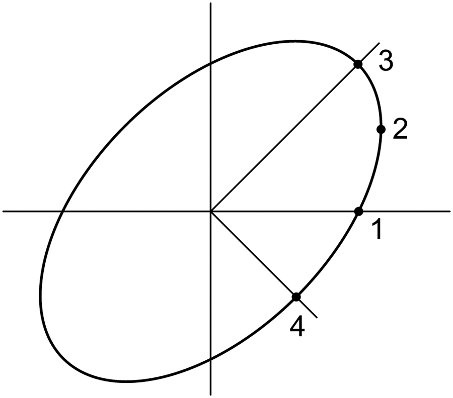
The von Mises yield criteria and yield stress values required for various stress paths.
In terms of uniaxial tension,
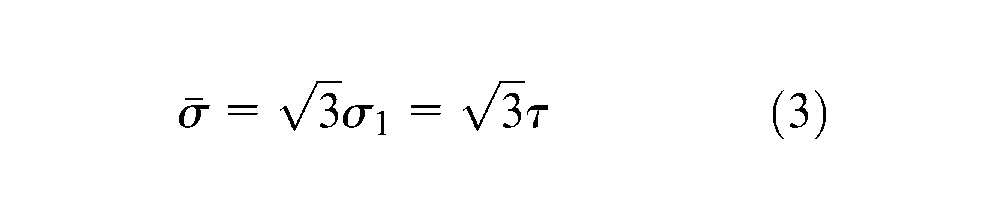
where
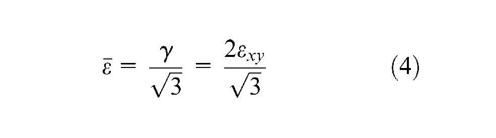
From this, we can see that the von Mises yield criterion enables us to derive the stress–strain curve of an equivalent tension–compression test by multiplying the shear stress in shear tests by the (conversion factor) and multiplying the shear strain by (2/conversion factor).
Then, based on the conservation of energy equation 13
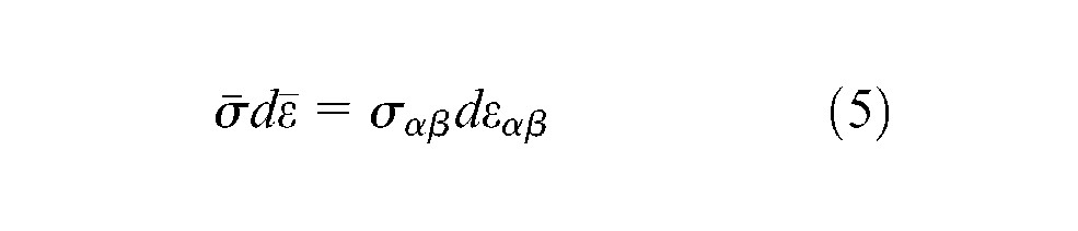
For shear tests, the equation for the conservation of energy is as follows
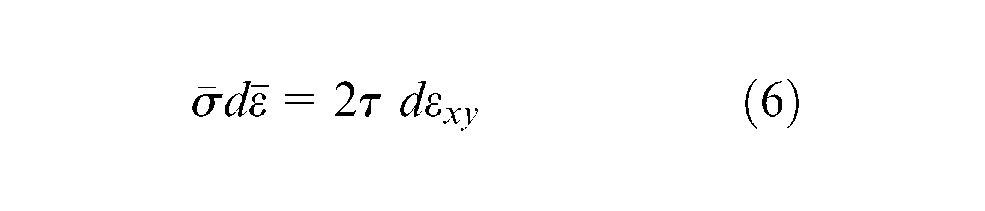
By substituting equations (3) and (4) into equation (6), we can see that the stress–strain conversion relationship observes the law of the conservation of energy.
Hill’48 yield criteria
The Hill’48 yield criteria are primarily applied to mild steel. In consideration of the anisotropy in the material, the equivalent stress is as follows
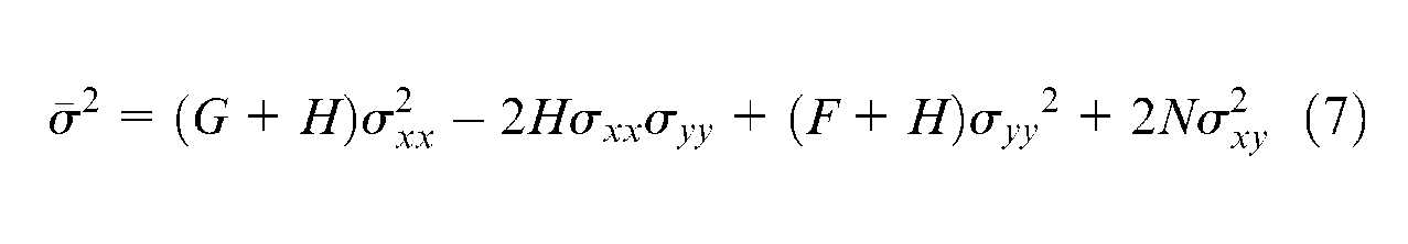
where
In shear tests,
The derivative of equivalent strain is
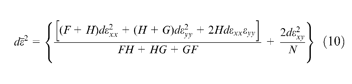
In shear tests,
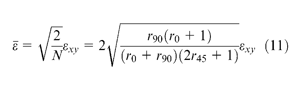
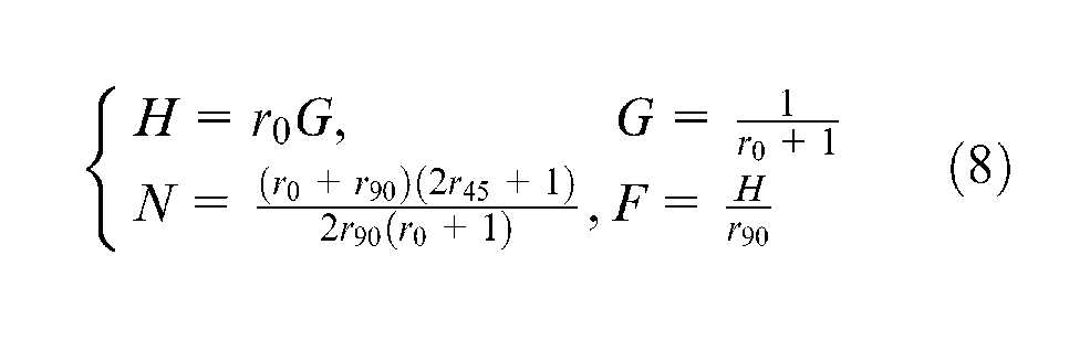
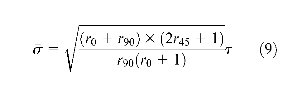
Equations (9) and (11) show that the conversion factor of the Hill’48 yield criteria is
Barlat’89 yield criteria
The Barlat’89 yield criteria are used mainly for materials with low anisotropic coefficients such as aluminum. The equation of equivalent stress is
where
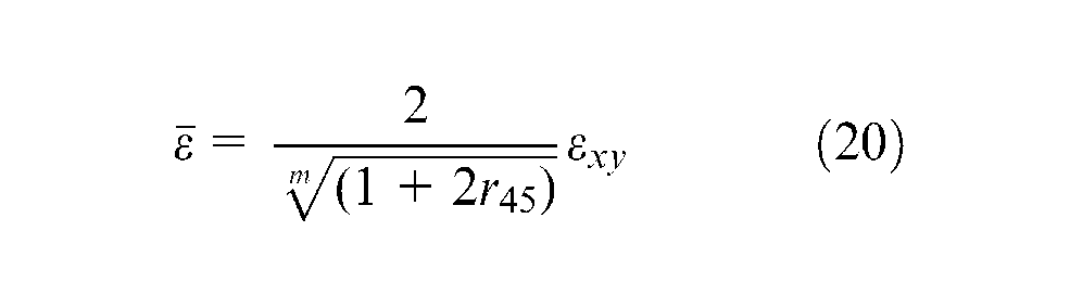
In accordance with the law of conservation of energy, we substitute equation (13) into equation (6) to obtain the conversion formula for equivalent strain
where
Furthermore,
Hill’90 yield criteria
The Hill’90 yield criteria are primarily applied to materials with low anisotropic coefficients such as high-strength steel. The formula for equivalent stress is as follows
or
where
Furthermore,
According to the equation for the conservation of energy, equation (6), we can derive that the equivalent tension stress is
where
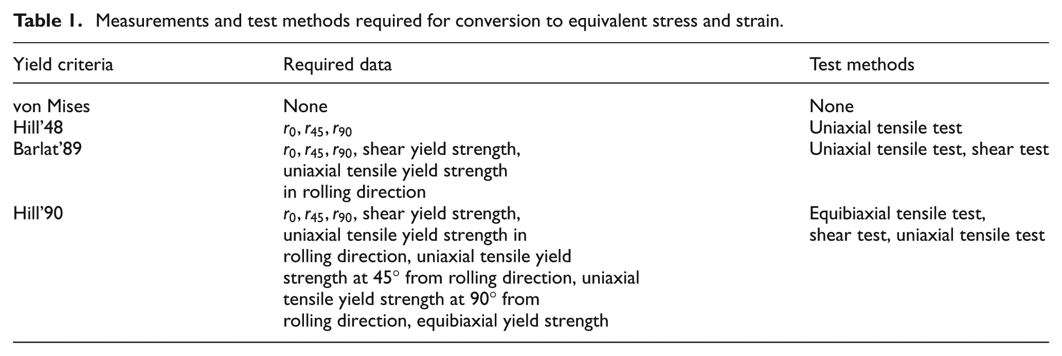
The test methods and measurement data required for each type of yield criteria are compared in Table 1, based on the above derivations related to equivalent stress and strain. As can be seen, the von Mises yield criterion does not require any measurement data. The Hill’48 yield criteria require only uniaxial tension tests to obtain the anisotropic coefficients at angles of 0°, 45°, and 90° from the rolling direction. The Barlat’89 yield criteria require shear tests to measure shear yield strength in addition to uniaxial tension tests. In addition to the tests mentioned above, the Hill’90 yield criteria require biaxial tension tests to measure equibiaxial yield strength, the equipment of which is sophisticated and expensive.
Measurements and test methods required for conversion to equivalent stress and strain.
Tension tests and calculation of YU model parameters
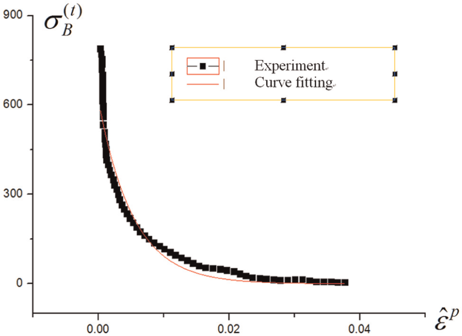
In reference to Shi et al., 4 this study used DP600 high-strength steel to conduct uniaxial tension tests and full cycle tension–compression tests. We used data capture software to capture the numerical data of the curves, as shown in Figures 2 and 4. Referring to the schematic diagrams for the YU model in Figures 3 and 5, we performed the following procedure:
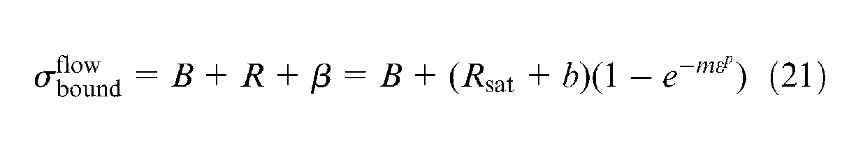
Using equation (21), we conducted curve fitting for the tension stage. Because the calculation results are associated with the adopted range of strain in the curve, we considered two curves with different ranges. In Case A, we captured a smaller strain range of 0.011–0.046; in Case B, we captured a larger range of 0.042–0.144. We then calculated the values for B, Rsat+b, and m
Referring to the upper and lower boundaries of the tension–compression tests in Figure 3, we obtained
By substituting b into the Rsat+b derived in Step 1, we obtained Rsat.
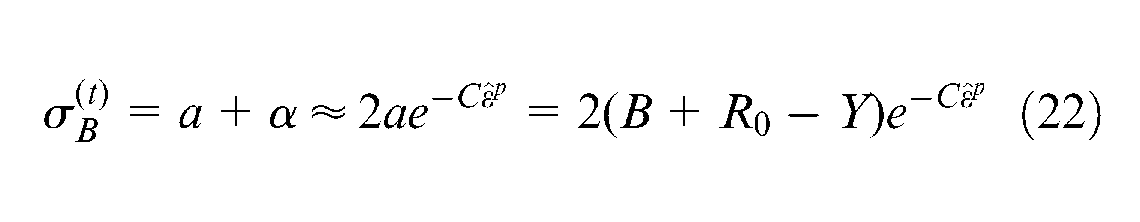
Referring to the transient Bauschinger effect curve in Figure 5 (the range between reyielding point and permanent softening), we obtained the experimental points for the region of transient Bauschinger effect as shown in Figure 4 and converted them into a
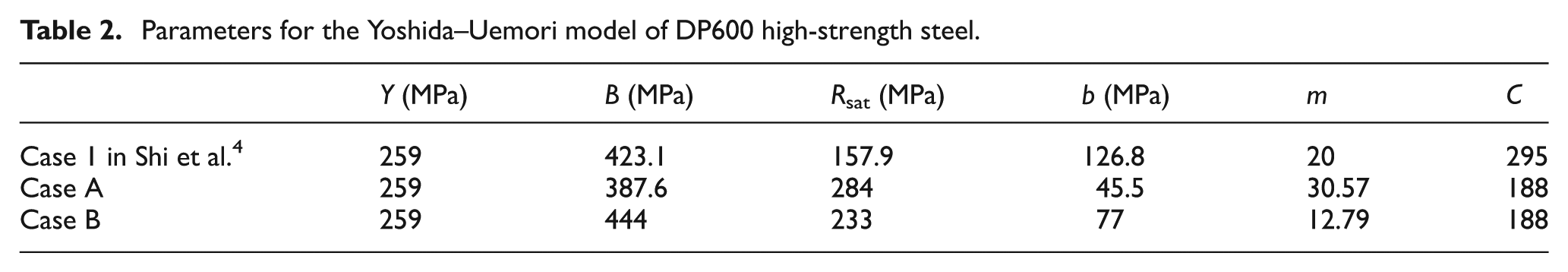
We employed the procedures above to obtain the parameters for the YU model in Case A and Case B, as shown in Table 2. Compared with the parameters obtained by Shi et al., 4 the results for Case B are closer to the reference values of Shi et al. 4
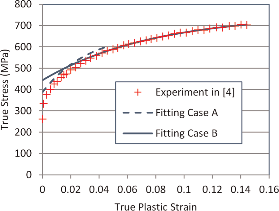
Uniaxial tension tests and curve fitting of DP600 high-strength steel.
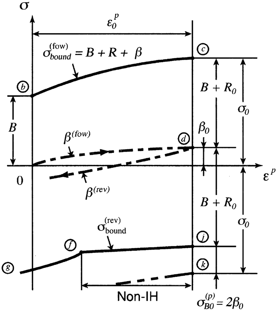
Schematic of upper and lower yielding boundaries of tension–compression tests in Yoshida and Uemori. 2
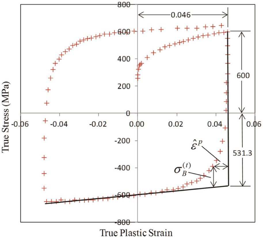
Full cycle tension–compression test curves of DP600 high-strength steel.
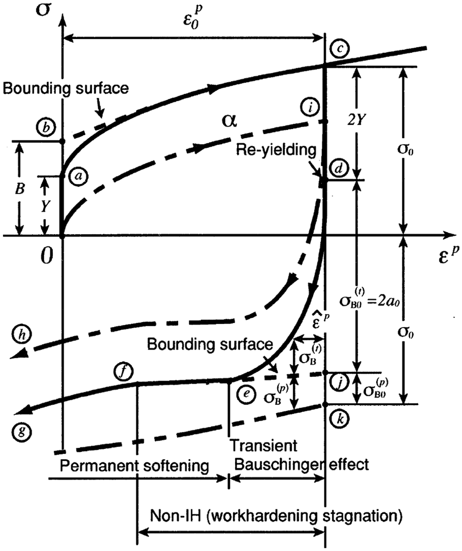
Schematic of transient Bauschinger effect region in tension–compression curve in Yoshida and Uemori. 2
Transient Bauschinger curve.
Parameters for the Yoshida–Uemori model of DP600 high-strength steel.
Verification of regression results for YU parameters in tension–compression simulation
To verify the parameters of the YU model obtained through regression, we used LS-DYNA to construct a tension–compression test model and used the MAT_125 material model to simulate the tension–compression tests. The stress–strain curve obtained was compared with the experiment and simulation results in Shi et al. 4
We divided a 10 × 10-mm-thin sheet into 100 square shell elements to represent the region of uniform deformation in an actual tension–compression test as shown as Figure 7. Thus, the analysis model constructed in this study simulates the process of uniform tension–compression deformation as closely as possible. Accordingly, we set the boundary conditions as follows: the middle point of the lower boundary fixes all degrees of freedom, and the remaining nodes in the lower boundary fix the uy, uz, rx, ry, and rz degrees of freedom. However, movement along the x-axis is allowed, which ensures that the nodes other than the middle point on the lower boundary are free to contract and expand along the x-axis. The nodes in the sheet were restricted from movement along the z-axis to prevent unnecessary warping, and the movements of the upper boundary along the y-axis were controlled to achieve the effects of tension–compression deformation.
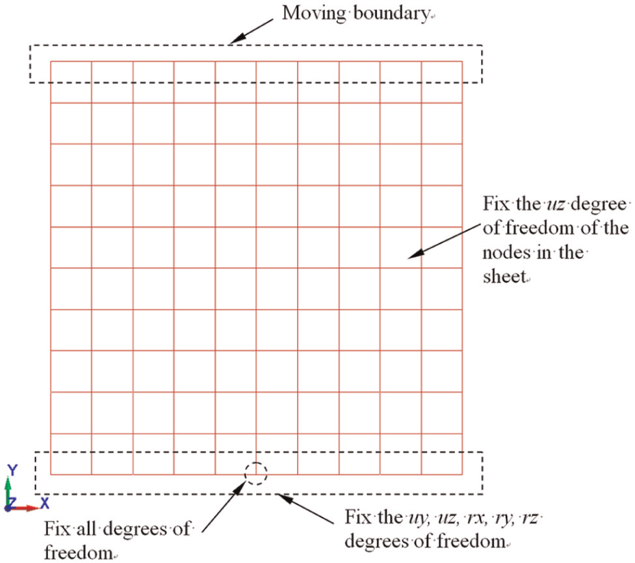
Finite element model for tension–compression test simulation.
Example 1: full cycle tension–compression test
Regarding parameters not mentioned in Shi et al.,
4
we used the DP600 settings in Ghaei et al.,
5
including the average anisotropic coefficients R = 0.905, Ea = 163e3 MPa, and
Figure 8 presents the regressed parameters in this study and the simulated parameter results in Shi et al. 4 in the full cycle tension–compression tests. By comparing the two sets of results, we discovered that the curve of Case A deviates entirely from the experiment results, rendering Case A inadmissible. The curve of Case B, however, is very close to the curve in the experiment as well as the curve derived by Shi et al., 4 with the exception of the portion in the second quadrant, which represents a partially deviation.
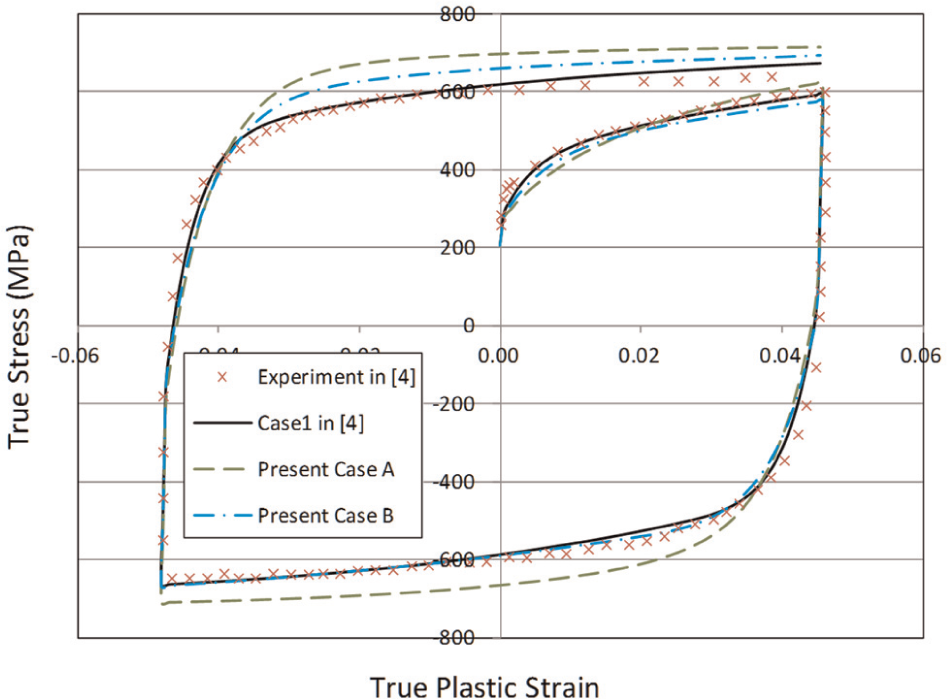
Comparison of the simulation results and experiment curve of Shi et al. 4 (full cyclic).
The h in the YU model represents the hardening properties of the material; h = 0 indicates isotropic hardening and h = 1 signifies kinematic hardening. As there is no theoretical method to derive h, a relatively more accurate h value could only be obtained by comparing the simulation and experiment curves of multiple h values.
In Figure 9, we modified the h value in Case B and observed whether adjusting the h value provided better results. When h = 0.9, we effectively lowered the curve in the second quadrant, bringing it closer to the experimental values; however, a portion in the third quadrant increased. Compared with the deviated curve in the second quadrant when h = 0.42, h = 0.9 still provided a better fit.
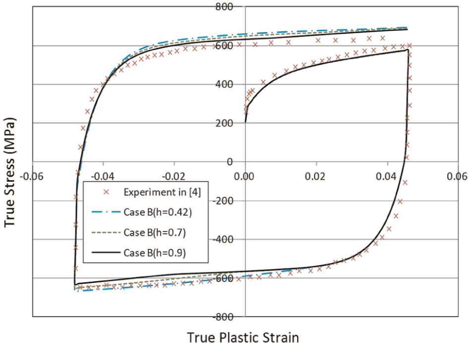
Influence of h values on results of Case B (full cyclic).
Example 2: single cycle tension–compression test
Figure 10 compares the regressed parameters in this study and the simulated parameter results in Shi et al. 4 in a single cycle tension–compression test. By comparing the two sets of results, we discovered that the curve of Case A deviates entirely from the results of the experiment, rendering Case A inadmissible. The curve of Case B, however, is very close to the experiment curve.
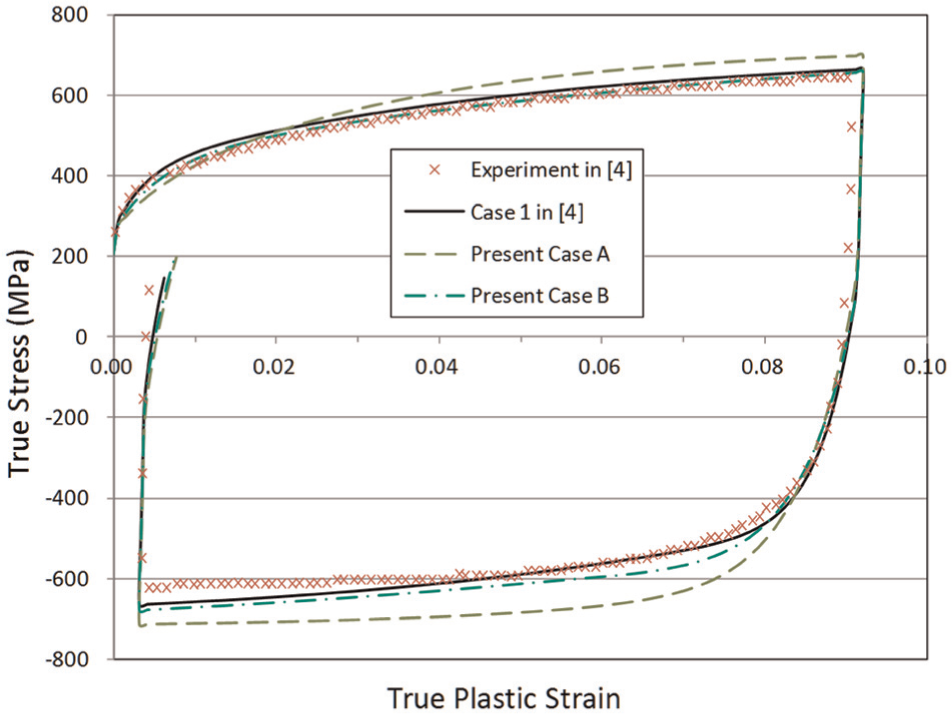
Comparison of the simulation results and experiment curve of Shi et al. 4 (single cycle).
In Figure 11, we modified the h value in Case B and observed whether adjusting the h value provided better results. When h = 0.9, the curve was closest to the experiment values, even closer to the experiment values than the results of Shi et al. 4
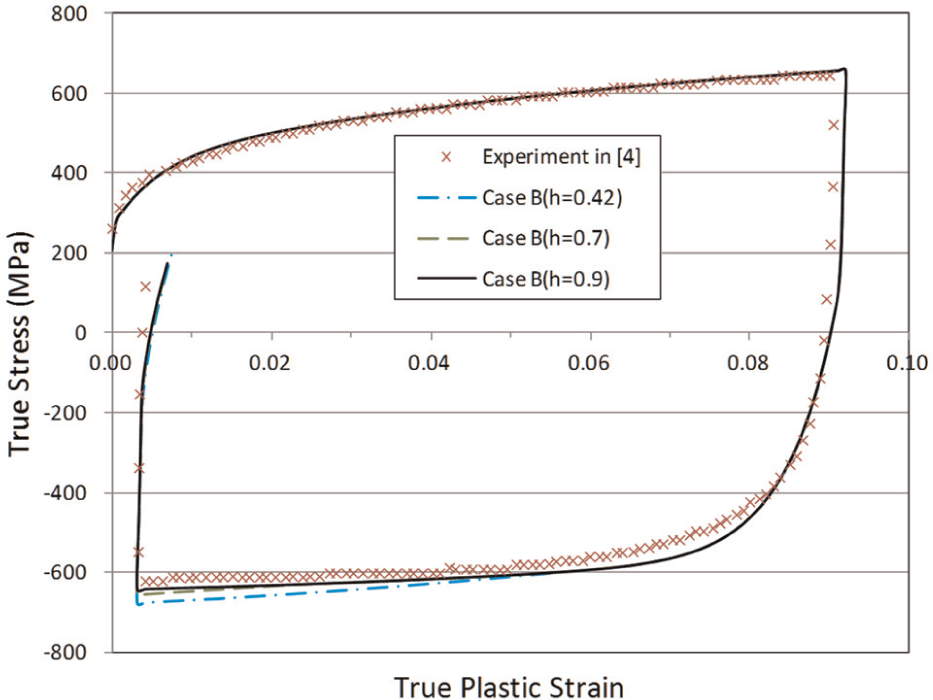
Influence of h values on results of Case B (single cycle).
From the two examples above, we can see that the parameters of the YU model derived through regression in this study are capable of simulating actual cyclic tension–compression tests. In addition, the parameter results of Case B, which employed a larger region of the tension curve, displayed significantly higher precision that those of Case A, which used a smaller region of the tension curve. Furthermore, in minutely adjusting h, we found that h = 0.9 presented a curve closest to the experimental results.
Shear tests and YU model parameter calculation
The experiment data obtained from Carbonnière et al. 14 are exhibited in Figure 12, showing the uniaxial tension curves and various forward and reverse shear test curves with various ranges of strain. The anisotropic coefficients of the sheet metal are r0 = 0.89, r45 = 0.88, and r90 = 1.12.
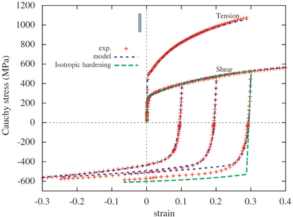
Uniaxial tension tests and forward and reverse shear tests of Carbonnière et al. 14
Using the conversion relationship mentioned previously, we employed the von Mises, Hill’48, and Barlat’89 yield criteria to convert the forward shear test curves into the uniaxial tension test curves as shown in Figure 13. Because the Hill’90 approach requires equibiaxial tension tests, the data of which are currently unavailable, we did not include this in the comparison. This figure shows that using the von Mises yield criterion results in a curve closest to the experiment results, whereas using the Barlat’89 yield criteria presented the greatest deviation from the experiment curve.
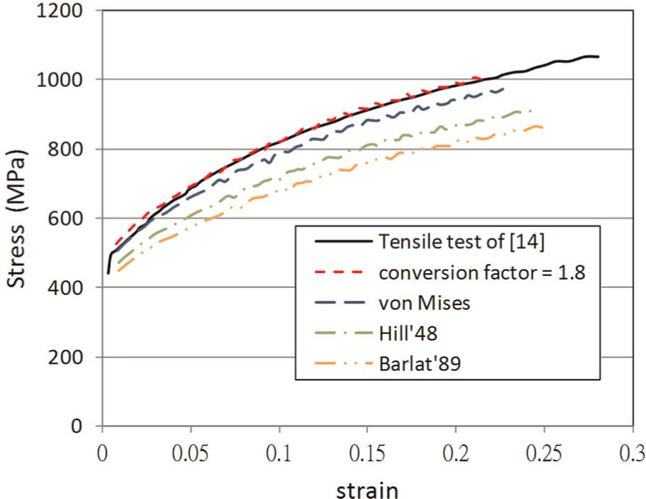
Comparison of converted forward shear test results with tension test curve of Carbonnière et al. 14
The equivalent tension test curves converted by these three methods still display significant differences from the actual tension test curve. To correct for the difference between the shear test curves and the tension test curves, we applied the law of the conservation of energy, multiplying the stress value in the shear tests by 1.8 and the strain values 2/1.8. In other words, the conversion factor was 1.8. The converted stress–strain curve was compared to the curves of the other three methods in Figure 13. Comparison results show that with a conversion factor of 1.8, the resulting equivalent tension test curve is very close to the uniaxial tension test curve.
We therefore adopted 1.8 as the conversion factor to transform the forward and reverse shear test curves into an equivalent tension–compression curve. The results are presented in Figure 14. Based on this curve, we calculated the parameters for the YU model, the results of which are listed in Table 3.
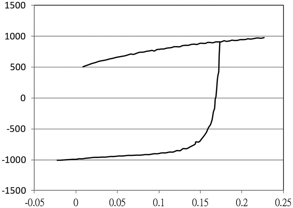
Equivalent tension–compression test curve converted using conversion factor of 1.8.
Yoshida–Uemori parameters of trip steel regressed from equivalent tension–compression curve.
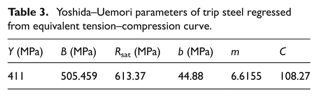
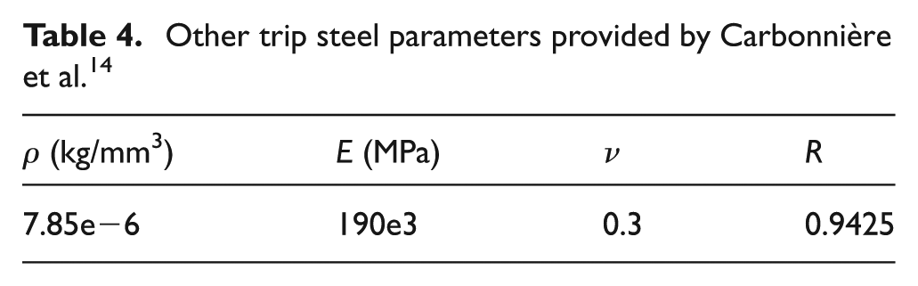
Table 4 shows the remaining trip steel parameters provided in Carbonnière et al. 14 As for Ea and ξ, we referred to the trip steel properties included in AUTOFORM, in which Ea = 104.55e3 MPa and ξ = 40.
Other trip steel parameters provided by Carbonnière et al. 14
Shear test simulation results and verification
We employed LS-DYNA to construct a numerical analysis model. We divided a 10 × 10-mm-thin sheet on the x–y plane into 100 square shell elements to represent the region of uniform deformation in an actual shear test as shown as Figure 15. The lower boundary fixed the degrees of freedom for the displacement of ux, uy, and uz, and the remaining nodes in the sheet fixed the degrees of freedom for the displacement of uy and uz. However, all the nodes allowed freedom in rotation, ensuring freedom in shear deformation in each element. The movements of the upper boundary along the x-axis were controlled to achieve the effects of shear deformation.
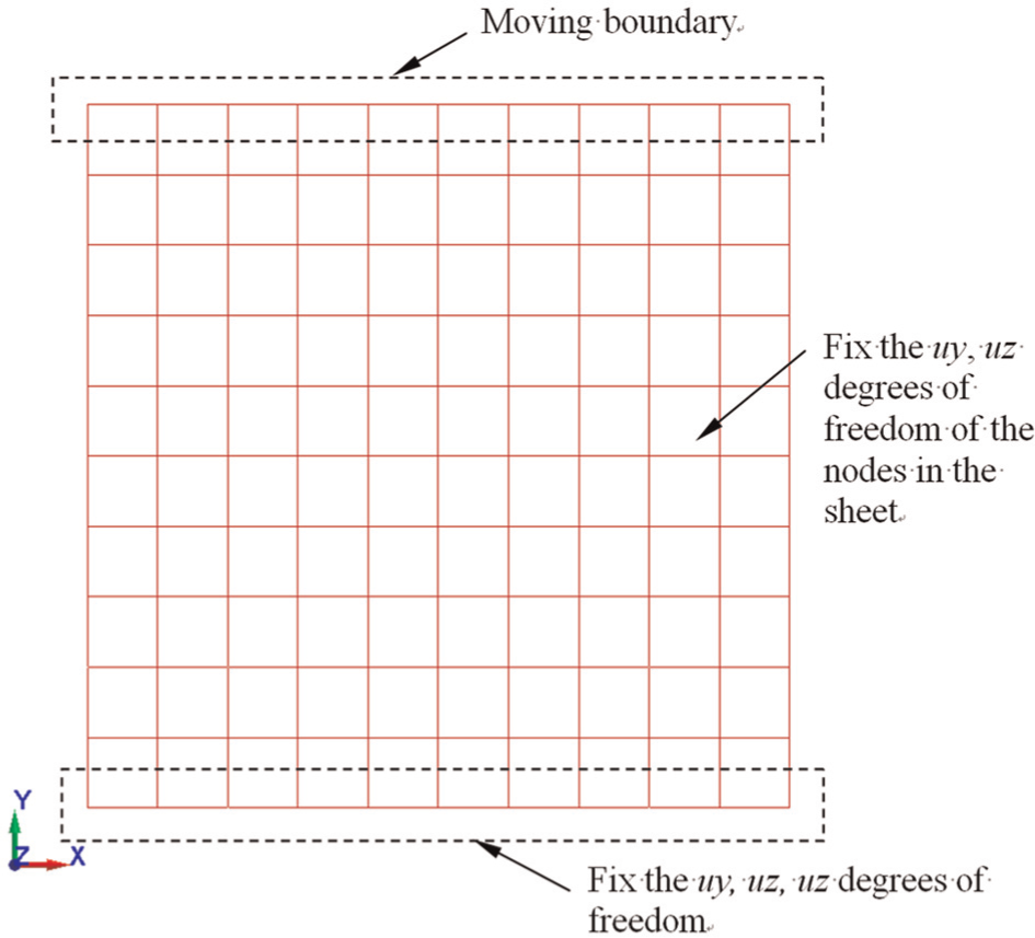
Finite element model for shear test simulation.
We first compared the forward and reverse shear tests with a maximum strain of 0.3. Considering various h values, we plotted the shear stress–strain curves and the experiment curve in Figure 16, in which h = 0.7 provided the curve closest to the curve in the experiment. Similarly, Figure 17 presents the curves for maximum strains of 0.1 and 0.2 when h = 0.7. A comparison with the experiment values revealed that with the exception of a few curve sections that deviated from the experiment curve, the great majority of the curve fit the experiment curve fairly well. This indicates that the proposed method of converting shear tests into equivalent tension–compression tests is feasible. Furthermore, the parameters for the YU model based on the equivalent tension–compression are applicable to the simulation of shear tests.
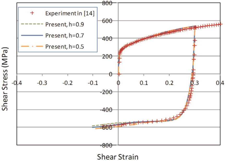
Influence of h values on shear test simulation curve.
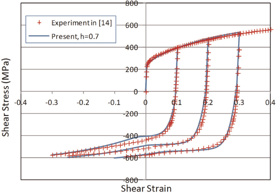
Comparison of trip steel shear test curve and simulation curve.
Conclusion
This study performed numerical regression to obtain parameters for the Yoshida–Uemori model. In both full cycle and single cycle tension–compression tests, the derived parameters accurately simulated experiment curves, according to a comparison with tension–compression experiment curves from the literature.
Shear tests provide the advantage of larger strain. This article proposes a methodology capable of accurately converting shear tests into equivalent tension–compression tests to obtain parameters for the YU model. Verification of these parameters using a numerical model demonstrates their applicability in the simulation of actual shear tests.
Existing theoretical models used to convert shear tests into equivalent tension–compression tests are still incomplete; however, by comparing the experiment curves of uniaxial tension tests and forward shear tests, we can derive a conversion factor capable of accurately converting shear tests into tension–compression tests. This study proposed a conversion factor of 1.8 for trip steel. The same method could also be applied to the conversion factors of other materials. This research team is currently constructing equipment for the shear tests and tension tests of high-strength steel to verify the applicability of the proposed conversion method.
Footnotes
Appendix 1
Declaration of conflicting interests
The authors declare that there is no conflict of interest.
Funding
This research received no specific grant from any funding agency in the public, commercial, or not-for-profit sectors.