Neural network–based modeling to predict residual stresses during electric discharge machining of Al/SiC metal matrix composites

Abstract

This article reports the result of an experimental study to analyze the effect of parameters that induce residual stresses during electric discharge machining of two particulate-reinforced metal matrix composites. Several factors were varied to study their impact on the formation of residual stresses, and pulse-off time was identified as the most significant factor. Artificial neural network was implemented to predict the residual stresses. Metal matrix composites with low coefficient of thermal expansion and high reinforced particle exhibit lower residual stresses. Also, better conductive electrode materials used during machining cause lower residual stress. The artificial neural network model accurately predicts the residual stresses and is a reliable tool for predicting residual stresses. The micrographs show that the workpiece with a higher concentration of reinforced particulates results in lesser flow line in the matrix material hence less residual stresses. X-ray spectra also reveal the phase transformation on the machined surface.

Introduction

Electric discharge machining (EDM) is a versatile machining process used for manufacturing variety of applications having stringent precision and accuracy requirements. In this process, the material is removed by a series of electrical sparks generated between two terminals (anode and cathode) in a dielectric medium. The process produces a mirror image of the tool (electrode) as it advances toward the workpiece. The process has the ability to machine hard-to-cut materials and can produce complex shapes. There are negligible cutting forces as there is no contact between the tool and work material resulting in a distortion-free and accurate machining with minimal requirement of manual skill. Because of this advantage, the EDM process is an attractive option to machine composite material such as particulate/fiber-reinforced metal matrix composites (MMCs) to achieve the required shape and size with superior dimensional accuracy and productivity. The temperature range of the spark developed is around 8000 °C–12,000 °C due to the excitation of a pulse generator, which produces rectangular shape pulses with adjusted on and off times, voltage level and discharge current. The sequence of sparks results in a substantial amount of phase transformation, thereby melting the surface of both poles. ¹ The efficiency of the machining process depends upon various process parameters such as spark energy, flushing pressure, dielectric medium and the electrode. During EDM of MMCs, a localized high-temperature electric discharge occurs in the presence of dielectric, which may result in change in mechanical and physical properties and also develop residual stresses within the material. The residual stresses affect the fatigue life of the workpiece and often cause distortion or cracking and, in some cases, also premature failure of the part in service.^2–5 For making this process commercially viable for MMCs, the prediction of induced residual stresses at various settings of input parameter is very important so that these could be controlled to improve the service life of the components. Developing a reliable mathematical model relating the machining parameters with residual stresses is very difficult due to complexities involved and also the nonlinearity of the EDM process. However, many researchers have reported the use of various neural network models to predict some responses accurately by effectively organizing the qualitative and quantitative factors. The work of McCulloch and Pitts ⁶ serves as the foundation for the growth of neural network architecture. The model suggested by them was further modified with the construction of electronic discrete variable automatic computer. ⁷ Currently, the most widely used artificial neural network (ANN) is multilayer perceptions based on back propagation (BP) techniques. The technique was employed for controlling and modeling various selected parameters. For example, many studies were feed forward BP to predict the surface roughness in machining processes.^8–11 Similarly, BP neural network control was used to predict tool wear and the resultant failures in drilling and turning operation.^12–14 Various neural network techniques have been used for prediction of responses during EDM.^15–17 Feed forward neural network with BP learning algorithm has been used to estimate the height of the workpiece online and distinguish the machining condition in wire EDM. ¹⁸ A process control system consisting of a fuzzy gap width controller adapted by neural network was introduced. ¹⁹ Experiments were conducted to develop a model of EDM using BP neural network with current, pulse-on time and pulse-off time as an input parameter for predicting the metal removal rate (MRR) and tool wear rate (TWR). ²⁰ A neural network was developed to study the steel transformation curve. ²¹ Feed forward neural network was used to classify the waveform generated from electrolyte-incorporated modified EDM. ²² Taguchi’s L18 orthogonal array was used to conduct experiments on explosive electric discharge grinding. The results were analyzed using genetic algorithm developed using neural network for optimization of the results. ²³ In another study, Taguchi’s L27 orthogonal array was used to present feed forward neural network based on BP along with a regression model to predict the surface roughness in abrasive jet machining process. ²⁴ The ANNs were applied successfully during machining and can accurately predict the responses during EDM.^25–29

The literature review shows that ANN is a powerful tool to develop models particularly in manufacturing applications to predict, generalize and analyze nonlinear multivariate data. Also, no study has been reported that applies ANNs to predict the induced residual stresses in particulate reinforced MMCs during EDM. In the present study, two types of particulate-reinforced Al MMCs were machined using EDM, and a superior and reliable process model was developed using ANN to predict the residual stresses.

Experimental study

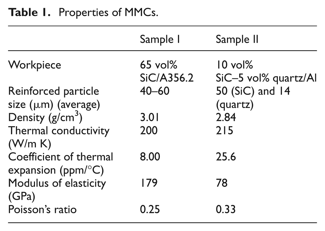
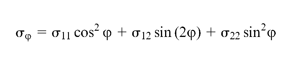
The experimental study was completed using two different types of MMCs commonly used for engineering applications. Material I (65 vol% SiC/A356.2 MMC) was procured in the form of a rectangular strip while material II was a hybrid (10 vol% SiC–5 vol% quartz in aluminum) prepared by stir casting method. The properties of both the materials are listed in Table 1. The experiments were conducted on a die sinking EDM machine (OSCARMAX SD550 ZNC, Taiwan) using conventional polarity. Three electrode (tool) materials namely (a) electrolytic copper, (b) fine grained graphite (particle size of 5.0 µm) and (c) copper–graphite composite with 50% Cu (Grade 673, resistivity: 2.03 µΩm and density: 2.95 g/cm³) procured from SGL Corporation, USA, were used to machine MMCs. A pilot study coupled with information available from the literature was used to identify the machine and process parameters to be varied during the study. Based on this study, current, pulse-on time, pulse-off time and dielectric fluid were identified for detailed study of their effect on residual stresses generated during machining. To draw valid conclusions from the experiments, each of these factors was varied at three levels to understand their impact on the development of residual stresses. Thus, a total of six factors namely material type (samples I and II), current (I), pulse-on time (t_on), pulse-off time (t_off), electrode material (I, II and III) and dielectric medium were chosen for study. The list of factors studied with their respective levels is shown in Table 2. The effect of these factors on normal stress (σ_φ) induced after machining of MMC samples was analyzed. Taguchi’s experimental design technique was used to design an orthogonal design from which valid conclusions could be drawn.^30–32 Considering the degrees of freedom required from the array, L18 was selected as the most appropriate array. The assignment of factors was carried out using MINITAB 15.

Table 1.

Properties of MMCs.

	Sample I	Sample II
Workpiece	65 vol% SiC/A356.2	10 vol% SiC–5 vol% quartz/Al
Reinforced particle size (µm) (average)	40–60	50 (SiC) and 14 (quartz)
Density (g/cm3)	3.01	2.84
Thermal conductivity (W/m K)	200	215
Coefficient of thermal expansion (ppm/°C)	8.00	25.6
Modulus of elasticity (GPa)	179	78
Poisson’s ratio	0.25	0.33

Table 2.

Factors interested and their levels.

Factors	Levels
	Level 1	Level 2	Level 3
Workpiece, w	65 vol% SiC/A356.2 (sample I)	10 vol% SiC–5 vol% quartz/Al (sample II)
Electrode, e	Cu	Gr	Cu–Gr
Current, I (A)	3	6	9
Pulse-on time, ton (µs)	10	30	50
Pulse-off time, toff (µs)	15	30	45
Dielectric, d	EDM oil (D)	EDM oil (D)+ Cu powder	EDM oil (D) + Gr powder

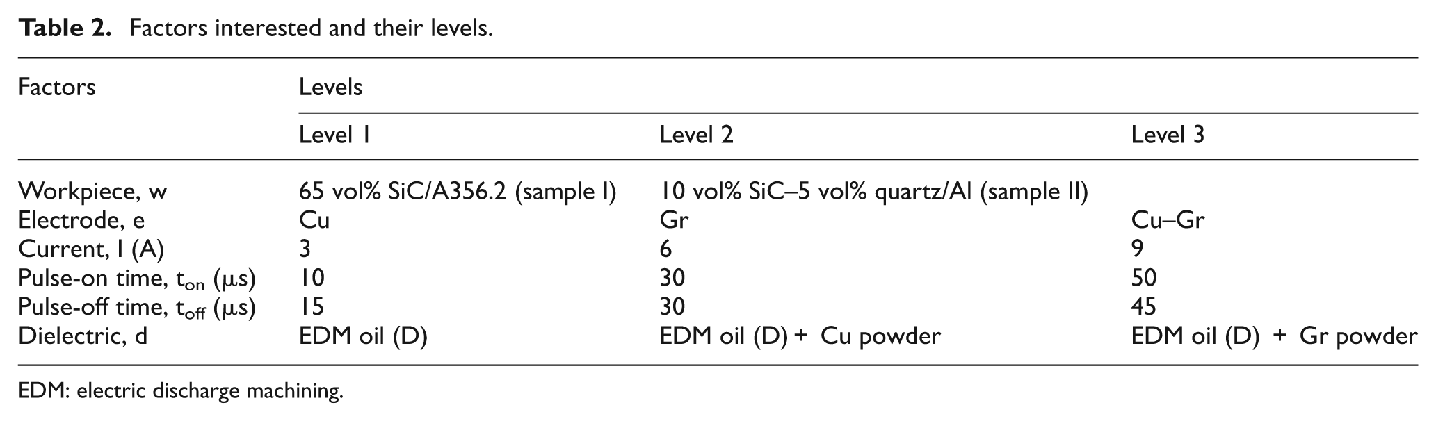
EDM: electric discharge machining.

Residual stresses

The component in service is subject to various types of stresses. The presence of residual stresses combined with external stresses may cause premature failures. The residual stresses are stresses, which are existing within a body/structure in the absence of external loading or thermal gradients. In other words, residual stresses in a body/structure are due to manufacturing methods, surface treatment, coatings, shot-peening process or structural change like phase transformation. X-ray diffraction (XRD) method used for measuring residual stresses in machined surface layer employs the characteristic radiation emitted from an X-ray. The advantage of this method is that repeated measurements are possible on the specimen. Figure 1 shows the schematic representation of concepts used in residual stress analysis.

Figure 1.

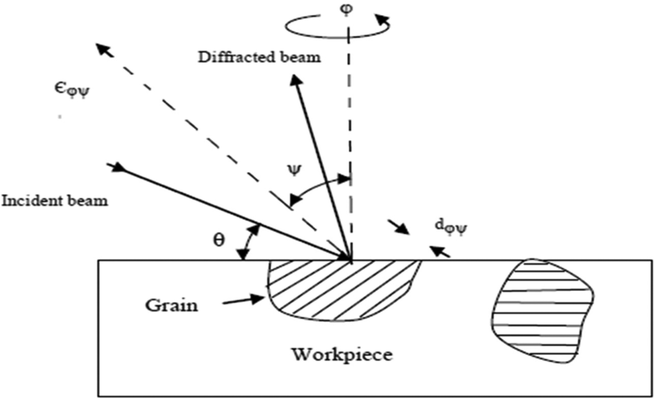
Concept of X-ray diffraction stress analysis.

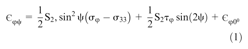
The general equation for measuring the residual stress is represented by equation (1). The lattice strain ${\in }_{\text{φψ}}$ is defined as ratio of the change in lattice spacing of atomic layer due to machining process to the un-machined lattice spacing tilted by ψ angle and rotated by ϕ angle of the sample

$${\in }_{\text{φψ}}=\frac{1}{2}{\text{S}}_2,\text{si}{\text{n}}^2\text{ψ}({\text{σ}}_{\text{φ}}-{\text{σ}}_{33})+\frac{1}{2}{\text{S}}_2{\text{τ}}_{\text{φ}}\text{sin}\left(2\text{ψ}\right)+{\in }_{\text{φ}{0}^0}$$

(1)

where

$${\in }_{\text{φψ}}=\frac{{\text{d}}_{\text{φψ}}-{\text{d}}_0}{{\text{d}}_0}$$

(2)

$${\in }_{\phi 0^0}=\frac{1}{2}{S}_2{\sigma }_{33}+{\text{S}}_1({\sigma }_{11}+{\sigma }_{22}+{\sigma }_{33})$$

$${\sigma }_{\phi }={\sigma }_{11}{\cos }^2\phi +{\sigma }_{12}\sin (2\phi )+{\sigma }_{22}{\sin }^2\phi$$

$${\tau }_{\phi }={\sigma }_{13}\cos \phi +{\sigma }_{23}\sin \phi$$

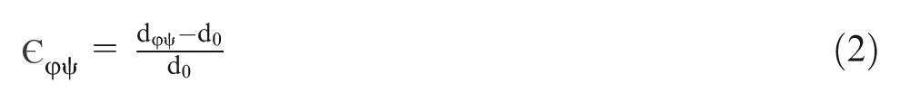
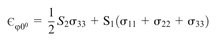
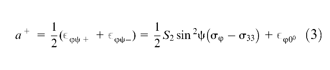
S₁ = −ν/E, 1/2S₂ = (1 +ν)/E, S₁ and 1/2S₂ are the X-ray elastic constants (XECs).^33–36 From equation (1), in order to measure the unidirectional normal residual stress, the parameter a⁺ is calculated using the lattice strain for positive and negative values of ψ for the particular rotational angle ϕ of the sample and is given by equation (3)

$$a^{+}=\frac{1}{2}({\in }_{\phi \psi +}+{\in }_{\phi \psi -})=\frac{1}{2}{S}_2\sin {\psi }^2({\sigma }_{\phi }-{\sigma }_{33})+{\in }_{\phi 0^0}$$

(3)

where ${\sigma }_{33}=0=0$ , ϕ = 0

During this study, the residual stresses induced during machining were measured using XRD method on PANalytical’s X’Pert Pro MPD (The Netherlands) diffractometer. The evaluation was completed using XRD classic technique using only one plane {hkl} to calculate the magnitude of residual stress. The machined surface was cleaned to remove the resolidified globules of molten metal to reduce measurement errors. In this experiment, the highest peak (2θ≥ 130°) also known as Bragg’s peak diffracted from the matrix phase of composite was selected for precise measurements. The small change in lattice spacing gives considerable change in peak angle, and it is represented by equation (4)

$$\frac{\Delta d}{\Delta \theta }=(-)\Delta \theta \cot \theta$$

(4)

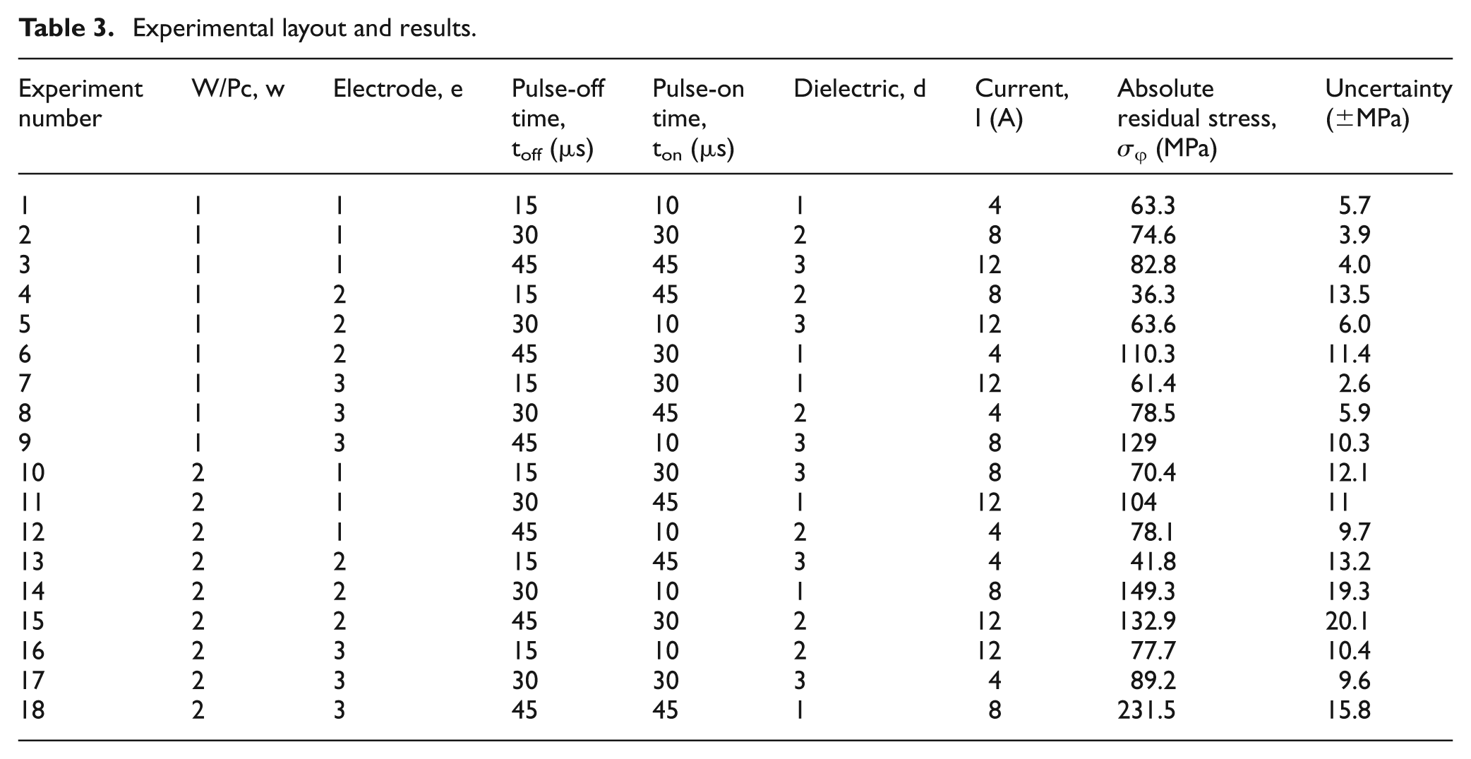
A number of independent XRD measurements of the isolated diffracted peak from the matrix phase of composite material were made at a different angle of ψ tilts. The obtained d_ϕψ spacing at different angles ψ tilt (positive and negative) was used to calculate the lattice strain. The calculated a⁺ was plotted against sin²ψ, and the slope of the linear fit curve was compared with equation (3). The residual stress with accepted uncertainty value due to the goodness of curve fitting was obtained. Sikarskie ³⁷ presented various factors contributing to the uncertainty in measurement of stress by XRD method. The inhomogeneous stress state generated during certain trials causes preferred orientation, which leads to lower peak intensities and less accurate peak location resulting in higher uncertainty. This effect of texture in measurement can be overcome by choosing appropriate tilts or translation of the sample to bring more grains in diffraction condition. The experimental layout and the measured residual stress values with uncertainty are shown in Table 3. The absolute residual stress (σ_φ) values with uncertainty were measured after each trial by above methodology and are given in the last column of Table 3.

Table 3.

Experimental layout and results.

Experiment number	W/Pc, w	Electrode, e	Pulse-off time, toff (µs)	Pulse-on time, ton (µs)	Dielectric, d	Current, I (A)	Absolute residual stress, σϕ (MPa)	Uncertainty (±MPa)
1	1	1	15	10	1	4	63.3	5.7
2	1	1	30	30	2	8	74.6	3.9
3	1	1	45	45	3	12	82.8	4.0
4	1	2	15	45	2	8	36.3	13.5
5	1	2	30	10	3	12	63.6	6.0
6	1	2	45	30	1	4	110.3	11.4
7	1	3	15	30	1	12	61.4	2.6
8	1	3	30	45	2	4	78.5	5.9
9	1	3	45	10	3	8	129	10.3
10	2	1	15	30	3	8	70.4	12.1
11	2	1	30	45	1	12	104	11
12	2	1	45	10	2	4	78.1	9.7
13	2	2	15	45	3	4	41.8	13.2
14	2	2	30	10	1	8	149.3	19.3
15	2	2	45	30	2	12	132.9	20.1
16	2	3	15	10	2	12	77.7	10.4
17	2	3	30	30	3	4	89.2	9.6
18	2	3	45	45	1	8	231.5	15.8

Sample calibration and data analysis for trial 6

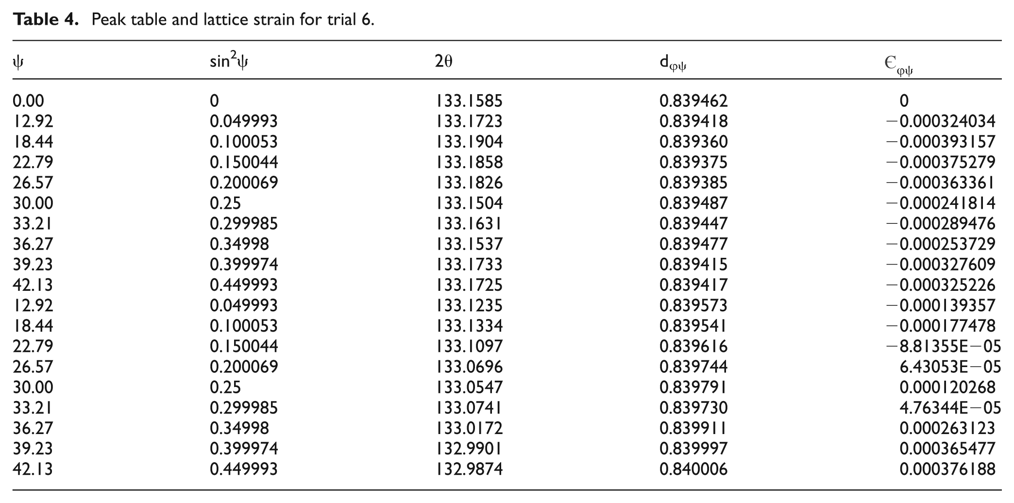
Residual stress was measured in matrix phase (Al phase) of the machined sample. The measurement is performed by selecting the isolated peak diffracted at the highest value of 2θ from {422} plane when using Cu Kα radiations (λ = 1.5406 Å). Table 4 for trial 6 (sample I) represents the change in lattice spacing measured from 19 ψ tilts. The calculated lattice strain for positive and negative ψ tilts is represented in the last column of Table 4. Residual stress was analyzed by comparing the linear fit regression equation obtained from the plot of a⁺ versus sin²ψ (Figure 2) with equation (3) as follows

Table 4.

Peak table and lattice strain for trial 6.

ψ	sin2ψ	2θ	dϕψ	${\in }_{\text{φψ}}$
0.00	0	133.1585	0.839462	0
12.92	0.049993	133.1723	0.839418	−0.000324034
18.44	0.100053	133.1904	0.839360	−0.000393157
22.79	0.150044	133.1858	0.839375	−0.000375279
26.57	0.200069	133.1826	0.839385	−0.000363361
30.00	0.25	133.1504	0.839487	−0.000241814
33.21	0.299985	133.1631	0.839447	−0.000289476
36.27	0.34998	133.1537	0.839477	−0.000253729
39.23	0.399974	133.1733	0.839415	−0.000327609
42.13	0.449993	133.1725	0.839417	−0.000325226
12.92	0.049993	133.1235	0.839573	−0.000139357
18.44	0.100053	133.1334	0.839541	−0.000177478
22.79	0.150044	133.1097	0.839616	−8.81355E−05
26.57	0.200069	133.0696	0.839744	6.43053E−05
30.00	0.25	133.0547	0.839791	0.000120268
33.21	0.299985	133.0741	0.839730	4.76344E−05
36.27	0.34998	133.0172	0.839911	0.000263123
39.23	0.399974	132.9901	0.839997	0.000365477
42.13	0.449993	132.9874	0.840006	0.000376188

$$0.000767=\frac{1}{2}{\text{S}}_2\left({\sigma }_{\phi }\right)$$

where 1/2S₂ = 6.98 T⁻¹Pa

Figure 2.

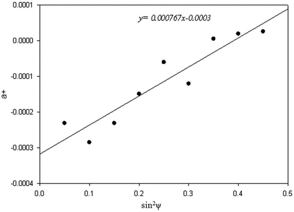
Represents a⁺ versus sin²ψ plot with regression equation of trail 6

Hence, the normal residual stress for trial 6 is 110 MPa with uncertainty of ±11.4 MPa

Results and discussions

The analysis of variance (ANOVA) for residual stresses induced into the machined surface was completed, and the results are given in Table 5. The factors with larger value of F-test indicate that there is a significant effect in inducing the residual stresses. Similarly, the p-value indicates the significance level for each factor. The contribution percentage of each input factor was measured by analyzing the F-value and the p-value. From the results, it is clear that pulse-off time is the most significant factor followed by dielectric medium, current, workpiece and electrode material. On the other hand, the effect of pulse-on time is negligible. For compressive, qualitative and quantitative analyses of EDM process, ANN was used to establish the relationship between input and output parameters and also to understand and predict the process performance. The main effect of various input parameters is presented in Figure 3.

Table 5.

Analysis of means for the residual stresses.

Factors	Degree of freedom	Sum of squares	Variance	F-value	p-value	Contribution (%)
W/Pc	1	4204.4	4204.4	9.13	0.023 a	10.436
Electrodes	2	3284.0	1641.98	3.57	0.095 a	6.586
Pulse-off time	2	14262.5	7131.27	15.49	0.004 a	37.188
Pulse-on time	2	110.5	55.26	0.12	0.889	Pooled
Dielectric	2	6526.1	3263.04	7.09	0.026 a	15.623
Current	2	4725.5	2362.75	5.13	0.050 a	10.604
Error	6	2762.6	460.44
Total	17	35875.7

a

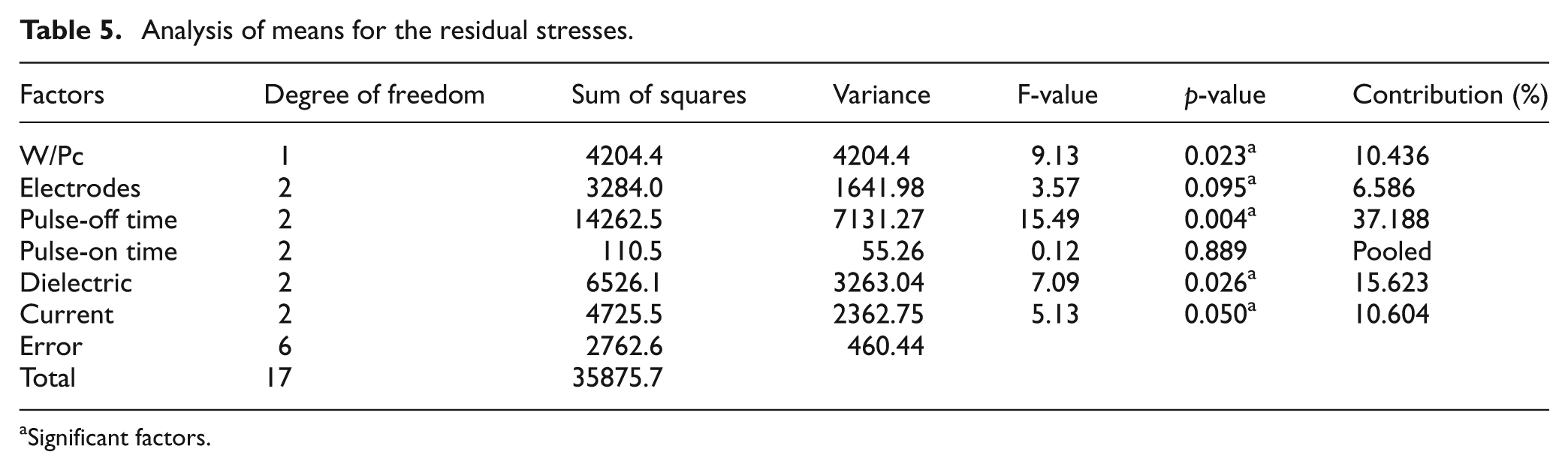
Significant factors.

Figure 3.

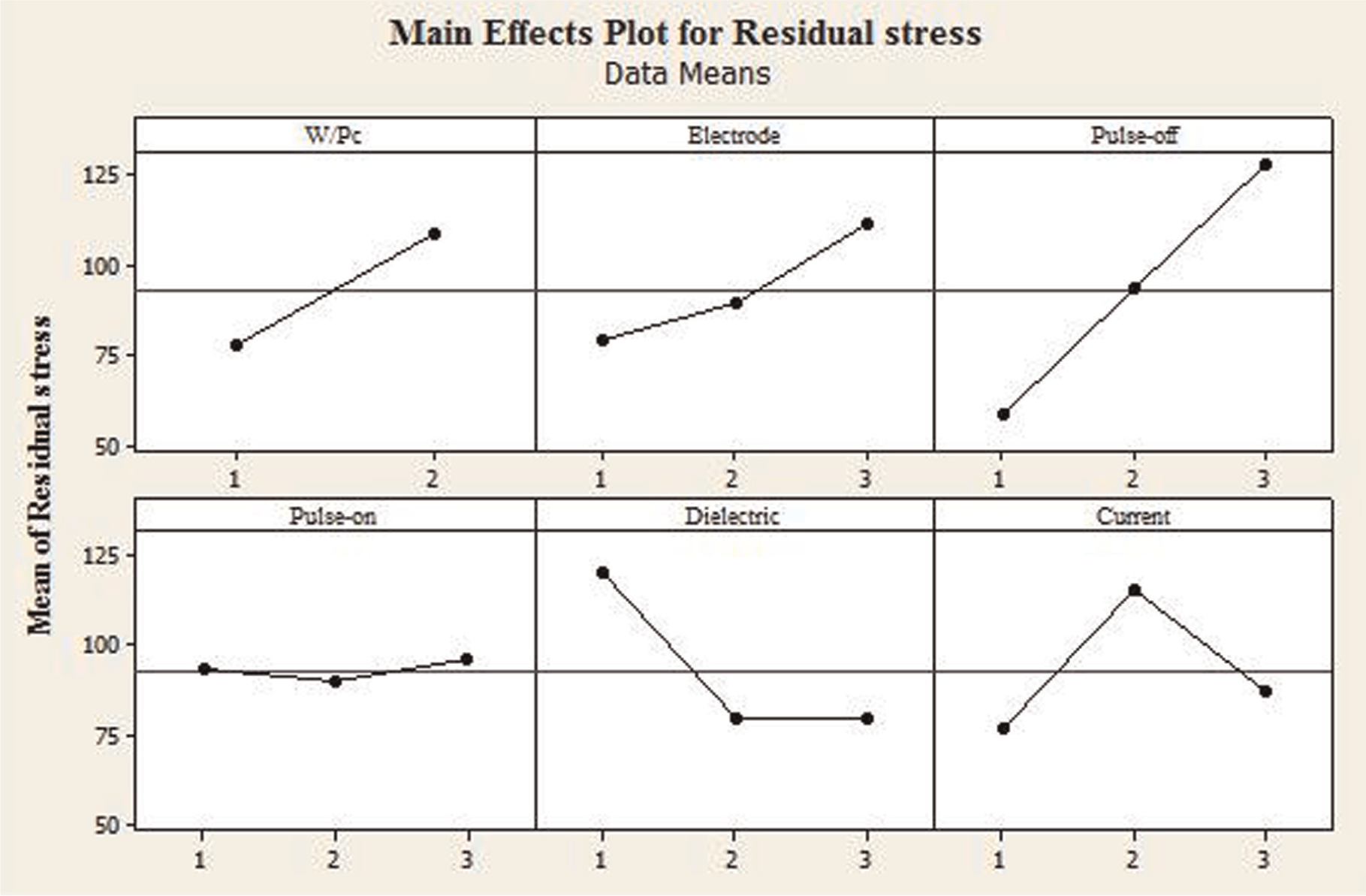
Main effect plots for residual stresses.

ANN

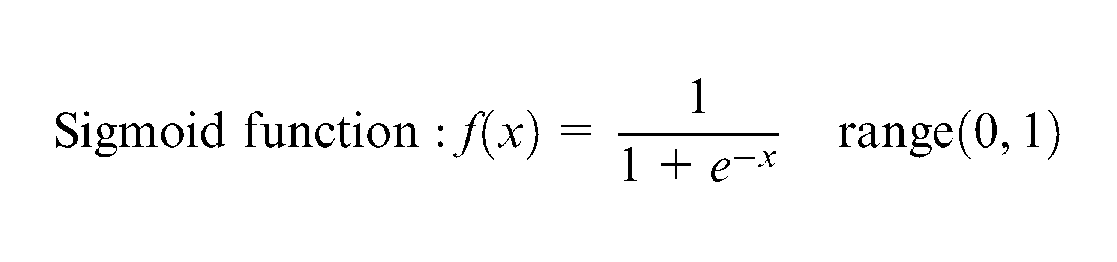
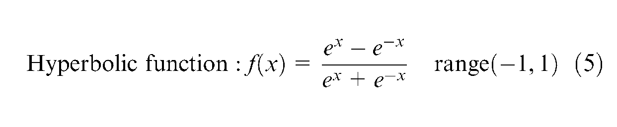
A feature borrowed from the physiology of the brain is the basis for the development of modeling technique known as ANN systems or simply neural networks. A neural network is defined by a collection of parallel processors connected together in the form of a directed graph, organized in such a way so that the network structure lends itself to the problem being considered. A network consists of processing element or unit in the network as a neuron, with connections between units indicated by the arc. The flow of information is indicated by the arrowhead on the connections. Figure 4 shows the general processing element or neuron model. Once the net input is calculated, it produces final output passing onto a nonlinear filter called activation function. There are several types of activation function used in neural network, but activation function mostly utilized in multilayer network is continuous in nature that varies gradually between the asymptotic values of 0 and 1 or −1 and +1 and is given by equation (5)

$$\text{Sigmoid}\text{function}:f\left(x\right)=\frac{1}{1+e^{-x}}\text{range}(0,1)$$

$$\text{Hyperbolic}\text{function}:f\left(x\right)=\frac{e^x-e^{-x}}{e^x+e^{-x}}\text{range}(-1,1)$$

(5)

Figure 4.

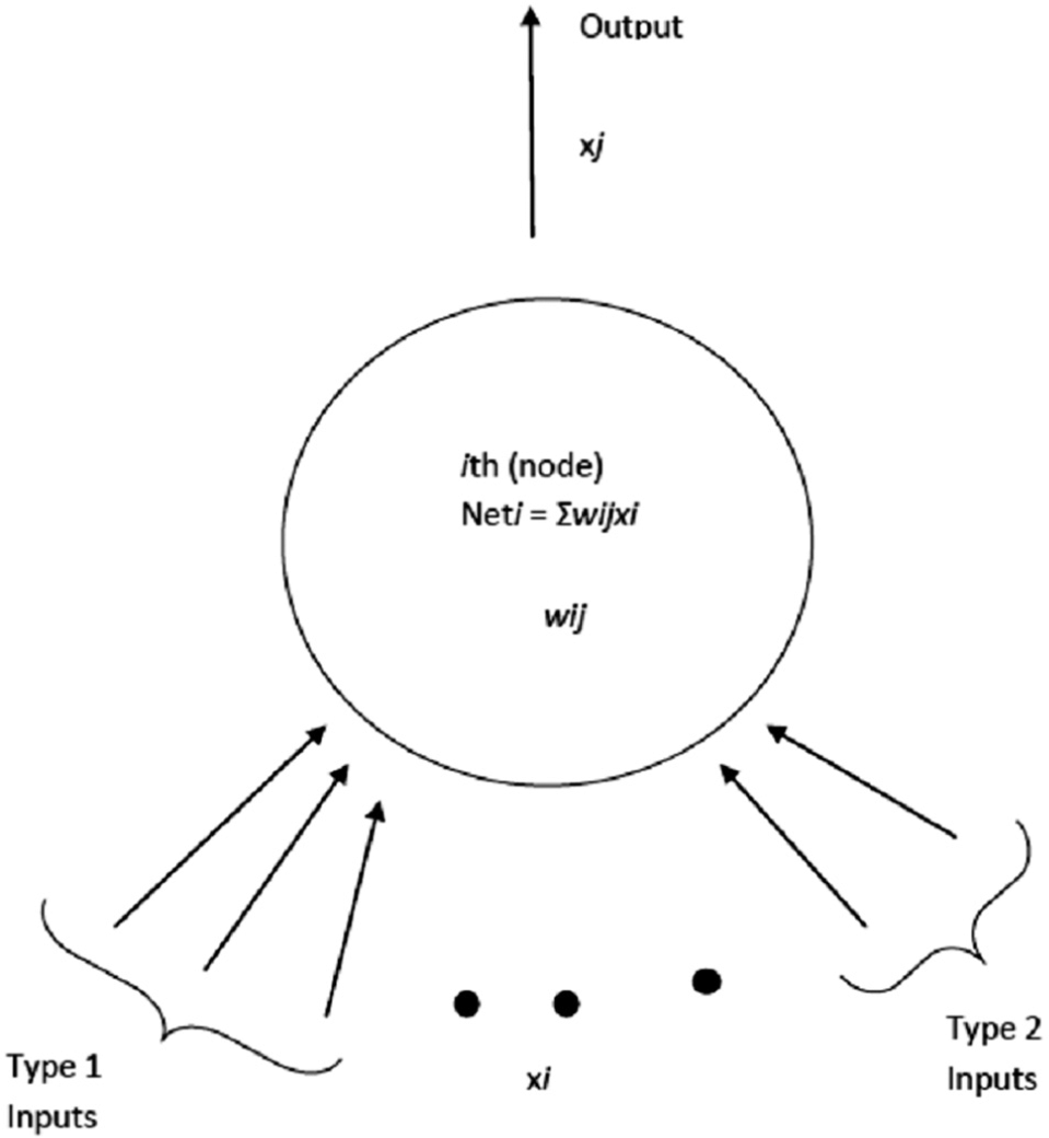
Schematic illustration of single neuron in a network. The input connections are modeled as an arrow from other nodes. Each input connection has associated with it a quantity wij, called weight.

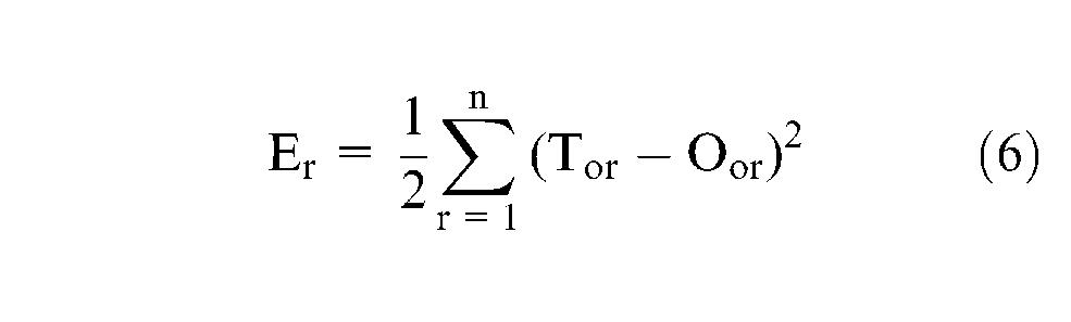
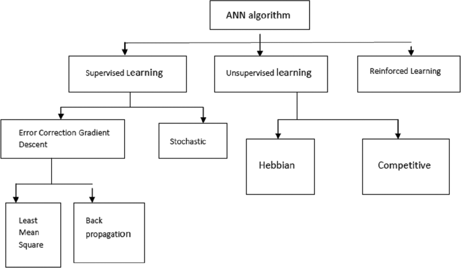
The identity function (f(x) = x) is available for the output layer neuron. The neural network is broadly classified into three basic types namely (a) supervised, (b) unsupervised and (c) reinforced, as shown in Figure 5. The BP method has been proven to be the most useful in manufacturing-related applications. The network learns from the predefined set of input–output example pairs using a two-phase propagate–adapt cycle. After the input pattern is applied as a stimulus to the first layer of network units, it is propagated through each hidden layers until an output is generated. This output is then compared to desired output, and an error signal is computed for output nodes. The difference between the output generated by network model (T_or) and the actual output (O_or) is given by equation (6)

$${\text{E}}_{\text{r}}=\frac{1}{2}\sum _{\text{r}=1}^{\text{n}}{({\text{T}}_{\text{or}}-{\text{O}}_{\text{or}})}^2$$

(6)

Figure 5.

Classification of learning algorithm.

Based on error signal, a connection weight is updated using BP algorithm.

Estimation of residual stresses by ANN

The estimation of model in neural network is composed of two stages: (a) training and (b) testing of the network with the experimental machining data. The network consists of one input, two hidden and one output layer and was assumed to be 6–n₁–n₂–1, where six are the input factors with 17 neurons in the input layer, n₁ and n₂ neurons in the hidden layer and one neuron in the output layer. The number of neurons in the hidden layer is determined by trial and error as there is no general methodology available to estimate these. The criterion is to select minimum number of nodes, which would not affect the performance of network by minimizing the storage memory for synaptic weight. When the number of hidden nodes is equal to the number of training patterns, the learning could be fastest but on the other hand, it loses the generalization capabilities. The error criterion adopted in the present model is sum of square error.

The procedure is outlined in the following:

• Divide the data set randomly in the training set and the testing set groups in appropriate percentage.

• Apply different network architectures to train the network.

• Evaluate the network architecture by comparing the normalized importance of each parameter obtained from the network with the ANOVA output results and percentage relative error.

• Test the network for its generalized ability using group of data classified for testing.

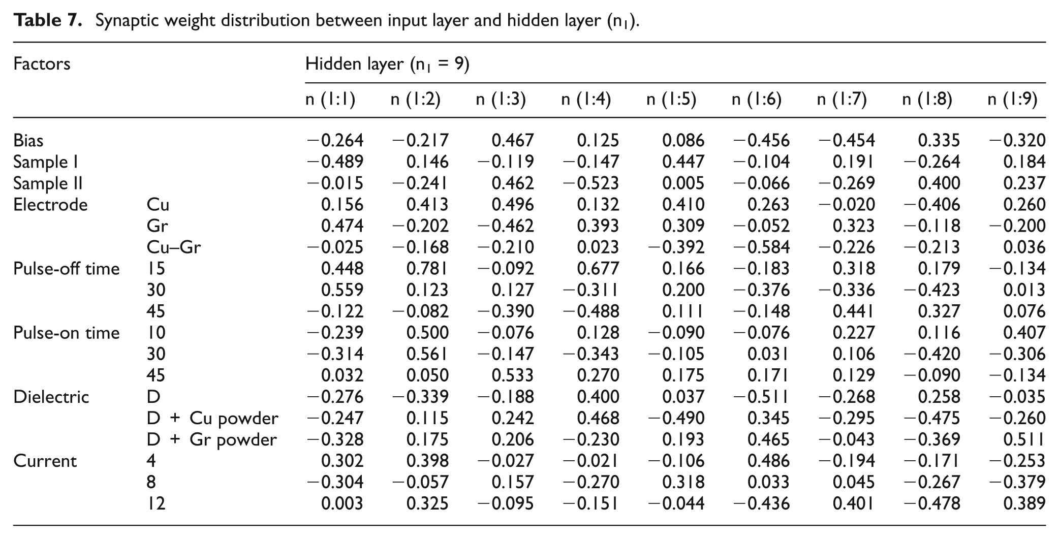
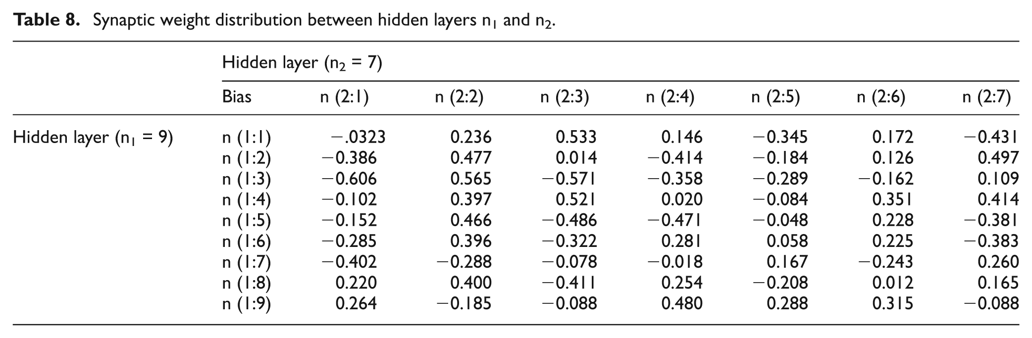
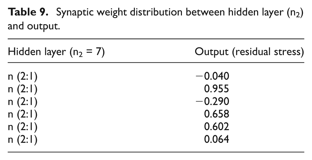
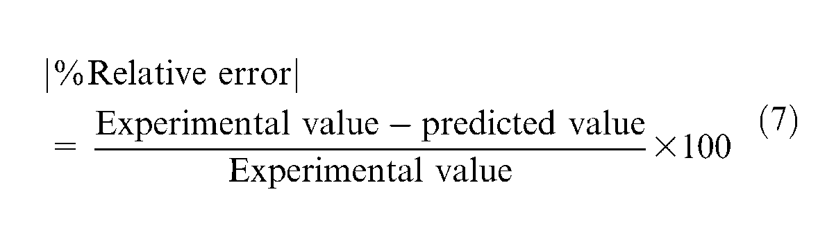
The experimental data given in Table 3 consist of 18 groups with the levels of input parameters/factors and residual stress as output response. Out of these, 12 group of data (given by trials 1, 2, 3, 5, 7, 8, 11, 12, 13, 15, 16 and 18) were randomly selected (about 67%) of all data groups were associated with training of network, and the remaining six groups of data (represented by trials 4, 6, 9, 10, 14 and 17) or 33% of data were used to test the network. For training of network, a commercial window–based ANN software, IBM-SPSS, was used. The number of network was constructed and the best network was selected based on minimum absolute relative error. This was interestingly achieved with first and second hidden layers having nine and seven nodes, respectively. The learning rate and the momentum values were selected as 0.001 and 0.7, respectively. The summarized neural network architect for the prediction of residual stress is shown in Figure 6. The weights were updated, and the activation function in hidden layers and output was selected as hyperbolic tangent and identity function, respectively. It was observed that the outcome of network directly depends upon the weight distribution done randomly. Thus, the network was trained repeatedly to update the weight until the hierarchy of normalized importance of each input parameter in the network showed consistency with the results obtained during ANOVA analysis. The results of neural network model are shown in Table 6. The synaptic weight distribution of the designed networks is shown in Tables 7–9. Also, it can be observed from Figure 7 that pulse-off time is the most significant factor followed by type of dielectric medium used. The other factors have relatively smaller significance with pulse-on time having the least significance. The performance of ANN was measured with absolute % relative error between the output of network with the experimental value and was calculated by equation (7)

Table 6.

Comparison of ANN model with experimental results.

Experiment number	Experimental response	ANN response	% Relative error
Training data
1	63.3	61	3.633491
2	74.6	75.4	1.07239
3	82.8	82.6	0.241546
5	63.6	64.5	1.41509
7	61.4	61.7	0.4886
8	78.5	78.1	0.509554
11	104	104.2	0.19231
12	78.1	80.1	2.56082
13	41.8	43.2	3.34928
15	132.9	132	0.677201
16	77.7	76.2	1.930502
18	231.5	233.1	0.69114
Testing data
4	36.3	56.6	55.3747
6	110.3	91.9	16.68178
9	129.0	142.1	10.155
10	70.4	74.9	6.39205
14	149.3	142.4	4.621567
17	89.2	78.6	11.88341

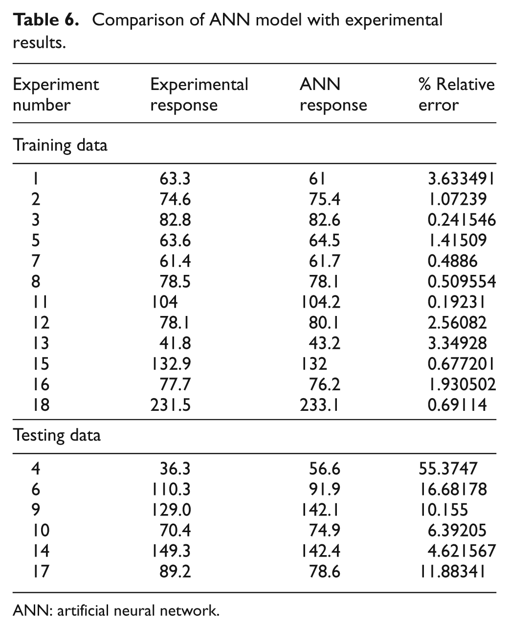
ANN: artificial neural network.

Table 7.

Synaptic weight distribution between input layer and hidden layer (n₁).

Factors		Hidden layer (n1 = 9)
		n (1:1)	n (1:2)	n (1:3)	n (1:4)	n (1:5)	n (1:6)	n (1:7)	n (1:8)	n (1:9)
Bias		−0.264	−0.217	0.467	0.125	0.086	−0.456	−0.454	0.335	−0.320
Sample I		−0.489	0.146	−0.119	−0.147	0.447	−0.104	0.191	−0.264	0.184
Sample II		−0.015	−0.241	0.462	−0.523	0.005	−0.066	−0.269	0.400	0.237
Electrode	Cu	0.156	0.413	0.496	0.132	0.410	0.263	−0.020	−0.406	0.260
	Gr	0.474	−0.202	−0.462	0.393	0.309	−0.052	0.323	−0.118	−0.200
	Cu–Gr	−0.025	−0.168	−0.210	0.023	−0.392	−0.584	−0.226	−0.213	0.036
Pulse-off time	15	0.448	0.781	−0.092	0.677	0.166	−0.183	0.318	0.179	−0.134
	30	0.559	0.123	0.127	−0.311	0.200	−0.376	−0.336	−0.423	0.013
	45	−0.122	−0.082	−0.390	−0.488	0.111	−0.148	0.441	0.327	0.076
Pulse-on time	10	−0.239	0.500	−0.076	0.128	−0.090	−0.076	0.227	0.116	0.407
	30	−0.314	0.561	−0.147	−0.343	−0.105	0.031	0.106	−0.420	−0.306
	45	0.032	0.050	0.533	0.270	0.175	0.171	0.129	−0.090	−0.134
Dielectric	D	−0.276	−0.339	−0.188	0.400	0.037	−0.511	−0.268	0.258	−0.035
	D + Cu powder	−0.247	0.115	0.242	0.468	−0.490	0.345	−0.295	−0.475	−0.260
	D + Gr powder	−0.328	0.175	0.206	−0.230	0.193	0.465	−0.043	−0.369	0.511
Current	4	0.302	0.398	−0.027	−0.021	−0.106	0.486	−0.194	−0.171	−0.253
	8	−0.304	−0.057	0.157	−0.270	0.318	0.033	0.045	−0.267	−0.379
	12	0.003	0.325	−0.095	−0.151	−0.044	−0.436	0.401	−0.478	0.389

Table 8.

Synaptic weight distribution between hidden layers n₁ and n₂.

	Hidden layer (n2 = 7)
	Bias	n (2:1)	n (2:2)	n (2:3)	n (2:4)	n (2:5)	n (2:6)	n (2:7)
Hidden layer (n1 = 9)	n (1:1)	−.0323	0.236	0.533	0.146	−0.345	0.172	−0.431
	n (1:2)	−0.386	0.477	0.014	−0.414	−0.184	0.126	0.497
	n (1:3)	−0.606	0.565	−0.571	−0.358	−0.289	−0.162	0.109
	n (1:4)	−0.102	0.397	0.521	0.020	−0.084	0.351	0.414
	n (1:5)	−0.152	0.466	−0.486	−0.471	−0.048	0.228	−0.381
	n (1:6)	−0.285	0.396	−0.322	0.281	0.058	0.225	−0.383
	n (1:7)	−0.402	−0.288	−0.078	−0.018	0.167	−0.243	0.260
	n (1:8)	0.220	0.400	−0.411	0.254	−0.208	0.012	0.165
	n (1:9)	0.264	−0.185	−0.088	0.480	0.288	0.315	−0.088

Table 9.

Synaptic weight distribution between hidden layer (n₂) and output.

Hidden layer (n2 = 7)	Output (residual stress)
n (2:1)	−0.040
n (2:1)	0.955
n (2:1)	−0.290
n (2:1)	0.658
n (2:1)	0.602
n (2:1)	0.064

$$\left|\%\text{Relative}\text{error}\right|=\frac{\text{Experimental}\text{value-predicted}\text{value}}{\text{Experimental}\text{value}}\times 100\text{}}$$

(7)

Figure 6.

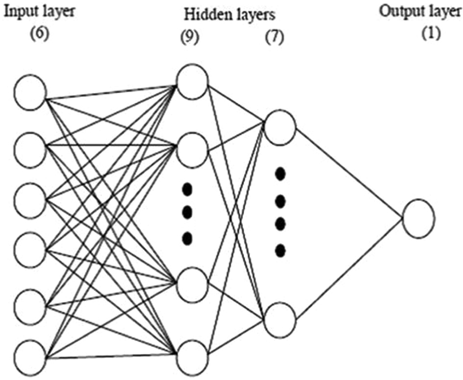
Neural network architect for residual stress calculation.

Figure 7.

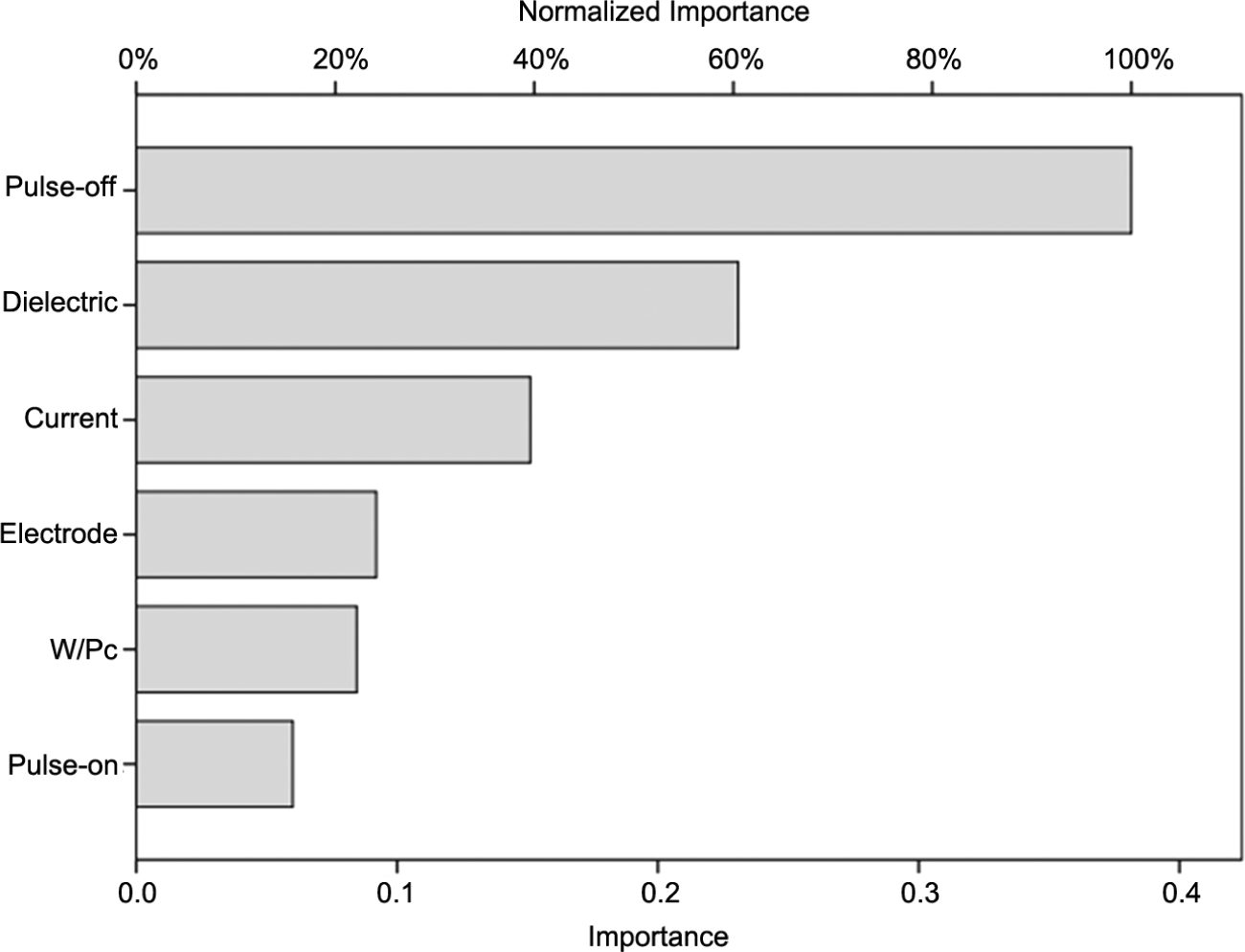
Normalized importance of each input factors on the residual stresses.

Figure 8 shows that the predicted data of network are very close to the experimental data results in verifying the network generalization capabilities.

Figure 8.

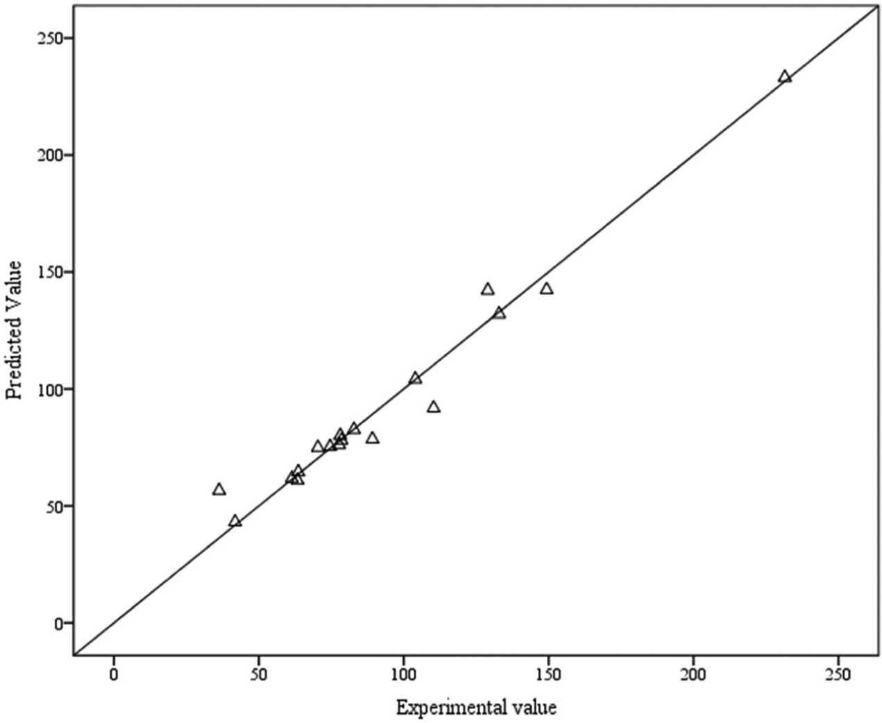
Comparison of ANN results and the experimental outputs.

Other statistical tools such as paired sample t-test and correlation were also completed to measure the amount of association between the experimental value and predicted value obtained from the network. The results are summarized in Tables 10 and 11. Table 10 shows that experimental value and the predicted value are positively correlated, r (N = 18) = 98.4%. Also, from Table 11, it can be concluded that the mean residual stress value increased from the experimental value to the predicted value by 0.227, t(17) = −0.119, p = 0.907 > 0.05. The experimental value and the results obtained from ANN model are not significantly different at 95% confidence range.

Table 10.

Correlation between the experimental value and ANN model value.

Variables	N	Mean	Standard deviation	Standard error mean	Correlation	Significance
Experimental value	18	93.039	45.9384	10.8278	0.984	0.000
ANN model value	18	93.266	44.9631	10.5979

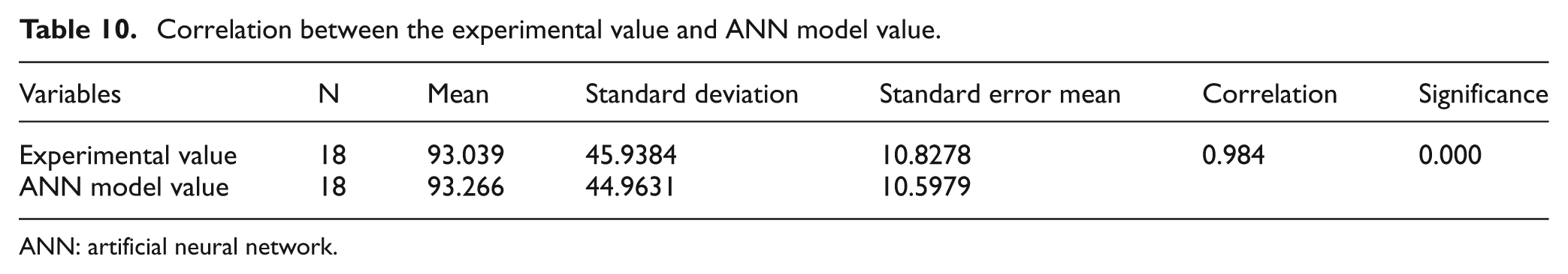
ANN: artificial neural network.

Table 11.

Paired sample t-test (experimental value and ANN model value).

Pair (N = 18)	Paired differences					t-test	Significance
	Mean	Standard deviation	Standard error mean	95% Confidence interval of the difference
				Lower	Upper
Experimental value and ANN model value	−.2273	8.1328	1.9169	−4.2717	3.8170	−0.119	0.91

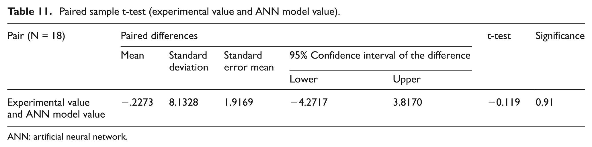
ANN: artificial neural network.

Microstructure analysis

For understanding the topography of EDMed surfaces in relation to the residual stresses induced during machining, a scanning electron microscope (SEM) study was completed on select samples for both materials used in this study. Figures 9 and 10 show the comparative residual stresses induced in materials I and II, respectively. Figure 9(a) shows the minimum residual stress in material I (65 vol% SiC/A356.2) obtained for trial 4 (I = 8 A; t_on = 45 µs; t_off = 15 µs, e = Gr, d = EDM oil + Cu powder). This may be because of a lower residual stress due to the pull out particulate and micro shrinkages, which are lesser deep. Similarly, the maximum residual stress for material I was obtained in trial 9, as shown in Figure 9(b) (I = 8 A; t_on = 10 µs; t_off = 45 µs, e = Cu–Gr, d = EDM oil + Gr powder). In this figure, the expelled material is resolidified on the workpiece in the form of globules leading to formation of micro cracks due to high energy level resulting in larger residual stresses.

Figure 9.

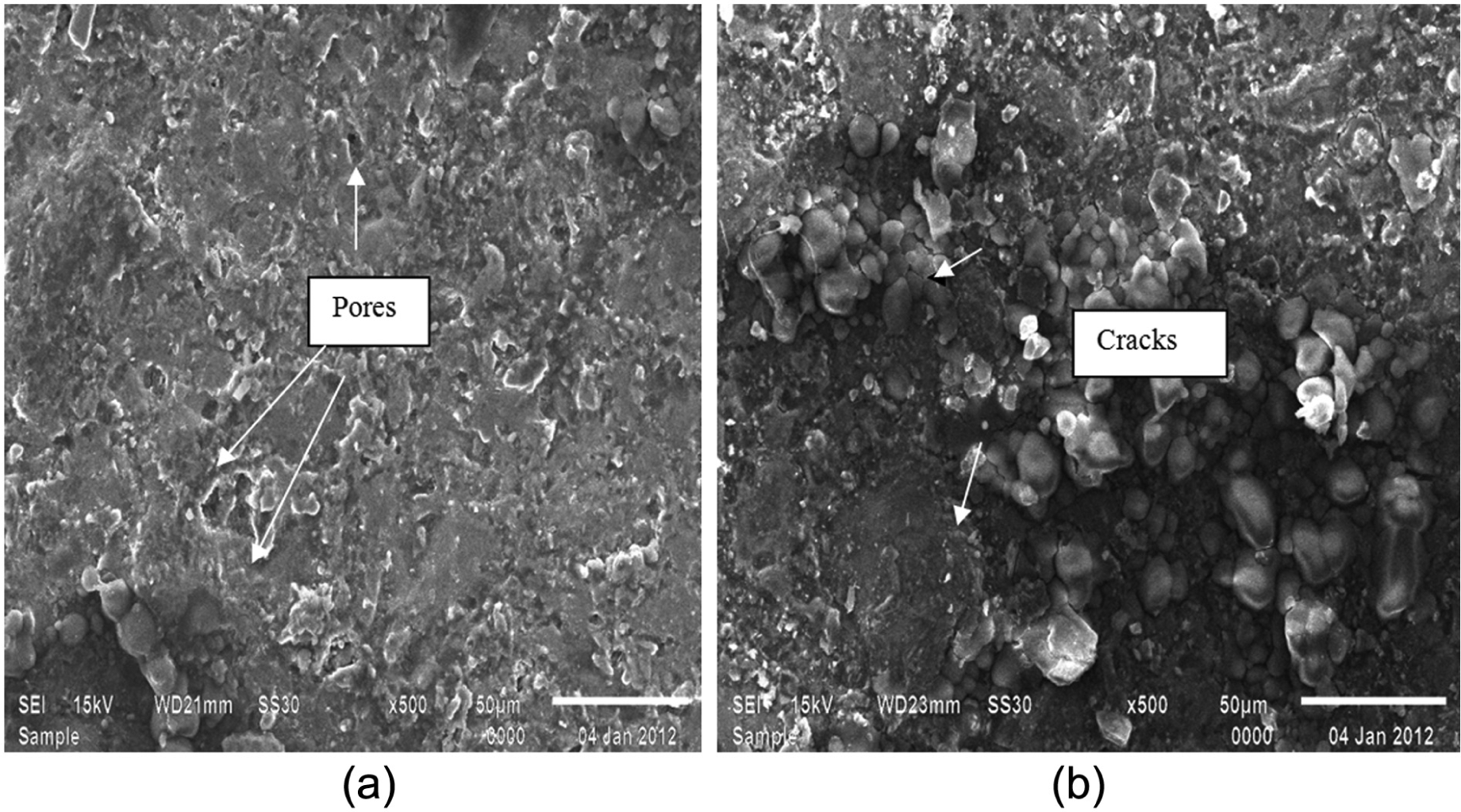
EDMed specimen of sample I: (a) residual stress = 36.3 MPa and (b) residual stress = 129 MPa

Figure 10.

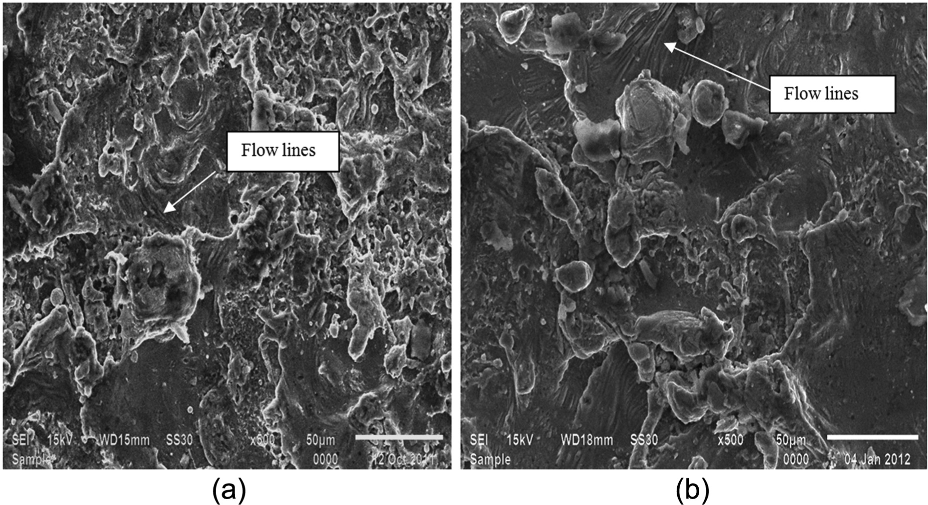
EDMed specimen of sample II: (a) residual stress = 41.8 MPa and (b) residual stress = 231.5 MPa.

Figure 10(a) and (b) shows the minimum and maximum residual stresses for material II (10 vol% SiC–5 vol% quartz/Al matrix composite). The minimum residual stress was obtained for trial 13 (I = 4 A; t_on = 45 µs; t_off = 15 µs, e = Gr, d = EDM oil + Gr powder), and maximum residual stress was obtained for trial 18 (I = 8 A; t_on = 45 µs; t_off = 45 µs, e = Cu–Gr, d = EDM oil). Both micrographs show the flow line of molten metal. However, these flow lines are more predominant in Figure 10(b) due to severe melting leading to high residual stress.

The SEM pictures of the machined surface represent the comparison of surface having highest and lowest residual stresses. This SEM analysis of the sample also reflects the surface properties of the machined surface such as surface roughness, porosity and crack. The machined surface in both the composites has a porous structure, which shows that the metal removal process was a result of melting, evaporation and spalling. ³⁸ Furthermore, the surface topography reveals that the residual stresses may be caused due to metal flow, globules pockmarks, voids and crack. For material I, the flow lines of molten matrix are not as severe as observed in material II due to low coefficient of thermal expansion and density of reinforced particulate but there is a formation of pores and voids in the micrograph.

Material I (65 vol% SiC/A356.2) does not show large flow line phenomena on the machined surface as seen in material II (10 vol% SiC–5 vol% quartz/Al composite). This could be due to low heat expansion coefficient and high density of reinforced particles in material I and thus do not experience high thermal gradient and volume change during EDM. The typical XRD spectra of un-machined and EDMed workpiece were carried out for both materials using Cu Kα radiations (λ = 1.5406 Å) to examine the changes on the machined surface using a scan rate of 1°/min and range up to 140° with the generator setting of 40 mA and 45 kV. The resulting scans are shown in Figures 11 and 12. The lower most plots in both figures are for the un-machined surface, and the other two plots are for trials, which exhibited lowest and the highest residual stresses. The XRD of machined surface in Figures 11 and 12 indicates the formation of new phases. The peak intensity reduces as the residual stress magnitude increases due to dislocation of planes of atoms.

Figure 11.

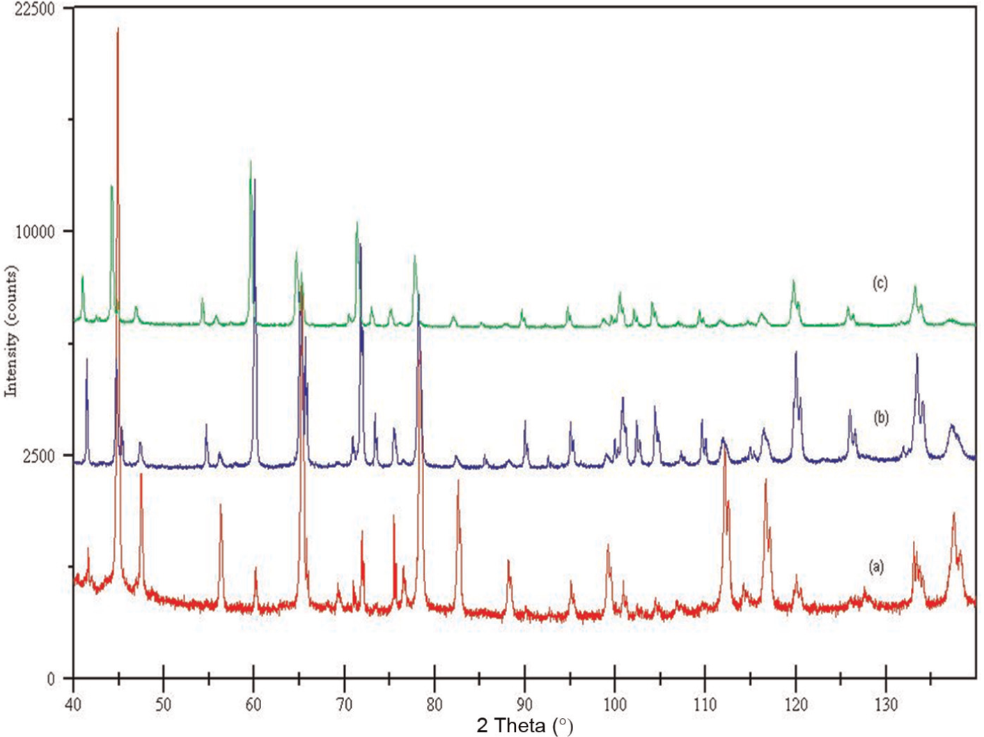
XRD spectra of sample I (a) before EDM and (b and c) EDMed surface with residual stress of 36.3 and 129MPa, respectively.

Figure 12.

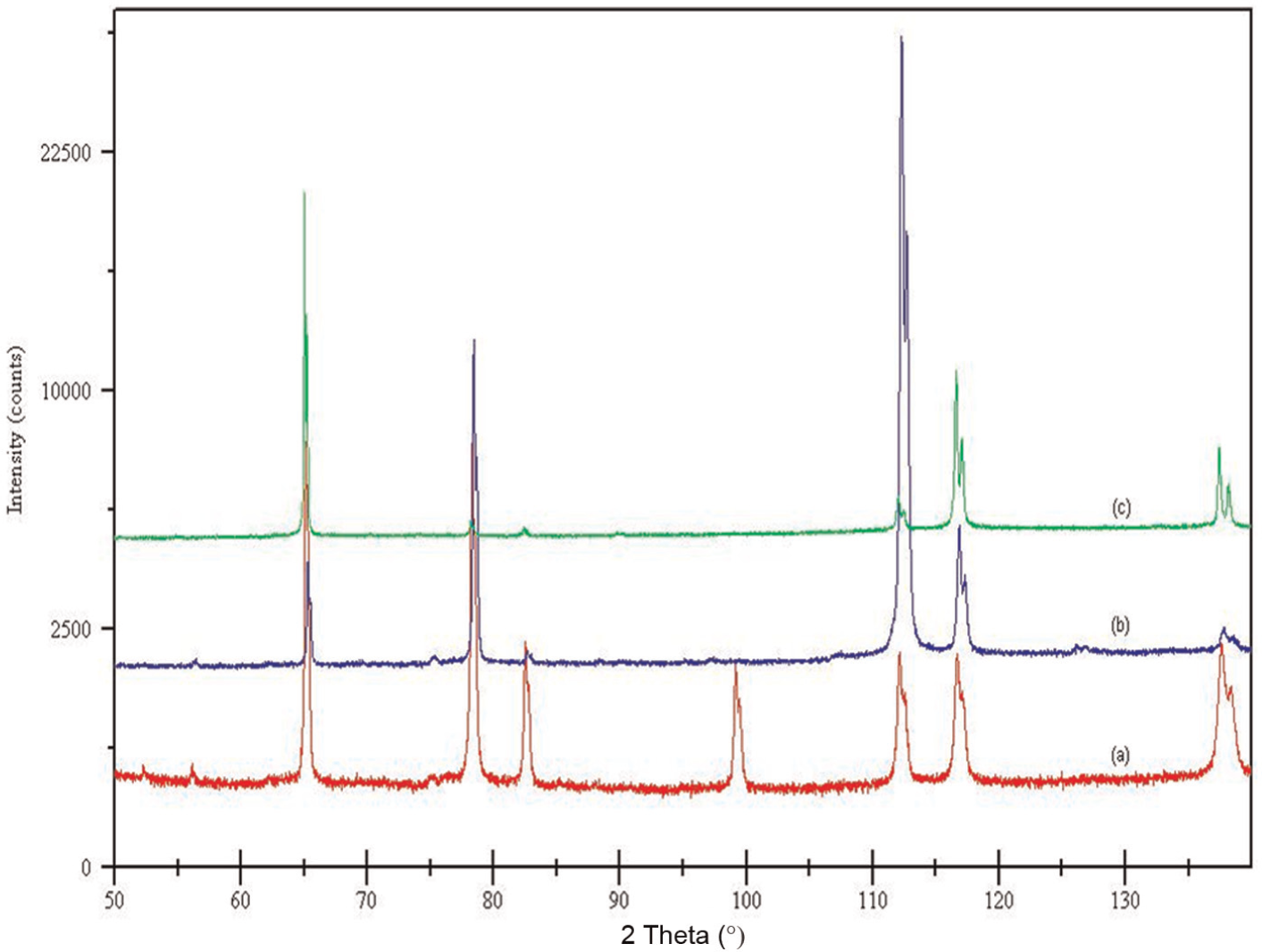
XRD spectra of sample II (a) before EDM and (b and c) EDMed surface with residual stress of 41.8 and 231.5 MPa, respectively.

Conclusion

This study reports the result of an experiment conducted on two different variants of MMCs for assessing the residual stresses induced while machining with an EDM process. Pulse-off time was identified as the most significant factor resulting in residual stresses in two materials. The analysis of results showed that MMCs with low coefficient of thermal expansion and a high density of reinforced particle have lower residual stresses. The electrode material which had high conductivity resulting in smooth formation of plasma channel between the electrodes induced least amount of residual stresses. The increase in pulse-off time causes a steep rise in residual stress due to extended solidification period while pulse-on time has no effect. The addition of power in the dielectric lowers the residual stresses. However, the conductivity of power particles has no effect on residual stresses. Subsequently, ANN model was developed to predict the residual stresses in such materials. The model accurately predicts the residual stresses and can be used as a reliable tool for the study of residual stresses in case of complex problems that involve qualitative and quantitative factors. The XRD patterns clearly indicate the formation of new phases on the machined surface. The peak intensity after machining is reduced due to dislocation of atomic layer resulting in residual strains.