
Abstract
Disassembly issues are important in the sustainable manufacturing field. One of them is influence factor analysis and time prediction of product disassembly. To deal with such issue, taking the bolt as a removal object, this work designs its removal experiment considering some factors influencing its removal process. Moreover, factor analysis and ranking on removal time are performed by a grey relational analysis method. In addition, based on the analysed and obtained main factors on removal time, its prediction models are established by multiple linear regressions, artificial neural networks and optimized artificial neural networks based on genetic algorithm methods. A numerical example is given to illustrate the proposed models and the effectiveness of the proposed methods.
Introduction
Due to stricter product recycling regulations, for example, Waste Electrical and Electronic Equipment (WEEE) Directive, and the higher awareness of environmental protection, recycling and remanufacturing issues for end-of-life products have raised the attention of the world. On the one hand, local government puts more efforts in policymaking of product recycling and remanufacturing.1–3 For example, in China, in order to enforce recycling and remanufacturing, some regulations are actively developed and implemented, that is, ‘Calculation method of recyclability and recoverability of road vehicles’ (2007) and ‘Recovery and management regulation on scrapped vehicles’ (2001). 4 On the other hand, some scholars have launched the discussion of their related issues. One of them is disassemblability analysis and design.
Gungor and Gupta 5 presented an evaluation and planning methodology to choose the best disassembly process among several alternative processes based on the total time for disassembly. Kroll et al.6,7 developed a method for quantifying the ease of disassembly. Its purpose was to advise designers to consider disassemblability for recycling from the beginning of design. Suga et al. 8 proposed a new method for the evaluation of disassemblability by introducing two parameters describing product disassemblability, namely, disassembly energy and entropy for disassembly. Mok et al. 9 presented a disassemblability analysis method for the recycling of mechanical parts in automobiles. The disassemblability analysis method include some important influence factors on product disassembly, for example, ease of fixing and ease of finding joining points, disassembly forces and disassembly directions. Desai and Mital presented a methodology to enhance the disassemblability of products. They defined disassemblability in terms of several influence factors on disassembly, namely, exertion of manual force for disassembly, degree of precision required for effective tool placement, weight, size, material and shape of components being disassembled and use of hand tools. Time-based numeric indices are assigned to each design factor. A higher score indicates anomalies in product design from the disassembly perspective.10,11 They developed a methodology to design products for disassembly incorporating ergonomic factors. 12 Chu et al. 13 presented economical green product design based on simplified computer-aided product structure variation. Mayyas et al. 14 and Vinodh et al. 15 addressed some disassemblability design issues on automotive products.
In addition, considering the impact of uncertainty factors on product disassembly, some disassemblability analysis methods dealing with the uncertainty management problem of product disassembly are presented. For example, Ilgin and Gupta16,17 presented a sensor-embedded product approach to detect missing components on disassembly uncertainty. Tian et al.18,19 defined some disassemblability evaluation parameters from the perspective of probability theory and established some probability evaluation models on disassembly process analysis. Tang and Zhou20,21 considered the uncertainty feature of disassembly time and quality of disassembled subassemblies in a disassembly process and analysed the expected disassembly cost and expected net profit of product disassembly based on the generic model for a human-in-the-loop disassembly system. They presented disassemblability analysis method considering human factors. Gao et al. 22 realized the intelligent decision-making of a disassembly process based on fuzzy reasoning Petri nets. Tang et al.23,24 discussed the uncertainty management issue based on the learning approach.
Based on the above overview, the current research mainly focuses on the integrated disassemblability analysis and design method incorporating one or multiple disassembly influence factors. In fact, to some extent, factors have a significant impact on the disassembly decision-making and design guideline of design for disassembly (DFD). Motivated by these, factor analysis issues on disassembly are probed. For example, Tang et al. 21 discussed the influence of operation fluency of human operators on disassembly using fuzzy logic. Shu and Flowers 25 investigated the selection issue of product life cycle fastening and joining methods from the perspective of design. Gungor 26 probed the evaluation issue of connection types in DFD using the analytic network process (ANP) method.
Although some researchers have proposed to use Fuzzy logic and ANP methods to address some influence factors on disassembly, they pay little attention to the grey analysis method and factor ranking issue of product disassembly. This work addresses influence factor ranking on component removal time based on a grey relational analysis (GRA) method. In addition, according to the obtained main influence factor, the prediction on component removal time is performed.
The rest of this article is organized as follows: Section ‘Removal experiment’ designs a removal experiment to obtain removal time. Section ‘Influence factors ranking on component removal time based on GRA’ presents the GRA-based influence factor analysis of component removal time. Section ‘Prediction of removal time’ describes some models to predict removal time and presents their prediction results. Finally, section ‘Conclusions’ concludes this article and describes future research issues.
Removal experiment
By taking the specified bolt of a transmission as an objective, this work obtains its removal times as presented in the following.
Removal objective and tools
Experimental objective
In this work, the M17 bolt of a transmission is taken as an objective to be removed, as shown in Figure 1. Its basic parameters are presented as follows: the bolt type is hexagonal, the maximum nominal diameter is 12 mm, the number of pitches is 12 and thread pitch is 1.82 mm.
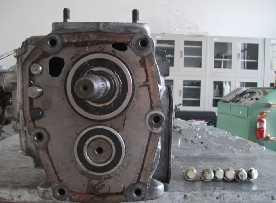
Schematic diagram of experimental objective.
Tools for removal
There are four types of tools used in this experiment, namely, wrench for tightening, wrench for removing, dynamometer and stopwatch. Wrench for tightening is used to fasten the bolt and demarcate the tightening torque of the bolt. Wrench for removing is a general ratchet wrench and is used to remove the bolt. Dynamometer is applied to measure the maximum tension of an operator. Stopwatch is used to measure the removal operation time of the bolt.
Experiment design and data acquisition
Experiment design
In the removal experiment, we consider only two factors, namely, the removal condition of the bolt and the quality of an operator. In terms of the removal condition of the bolt, it is simulated by the tightening torque of the bolt. It is demarcated by three levels, namely, 25 N m, 50 N m and 75 N m. Note that Newton metre (N m) is the unit of torque.
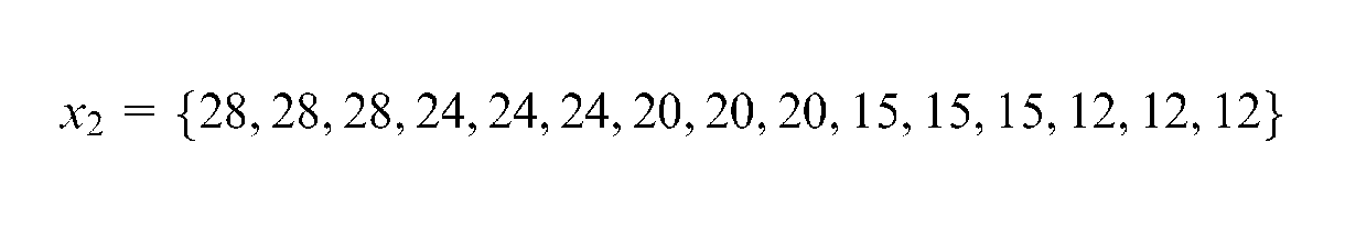
In terms of the quality of operators, during the removal experiment, since five skilled ones are selected, their operation fluency is considered as being high. Based on this premise, the quality of operators is determined by their maximum tension. Each maximum tension can be obtained by the tension experiment. Usually, the larger the maximum tension of an operator, the better its ability of disassembly and the smaller the needed disassembly time to disassemble a product.
In this experiment, it is demarcated by five levels, namely, 28 kg f, 24 kg f, 20 kg f, 15 kg f and 12 kg f. Note that kilogram force (kg f) is the unit of tension, 1 kg f = 9.8 N.
Data acquisition
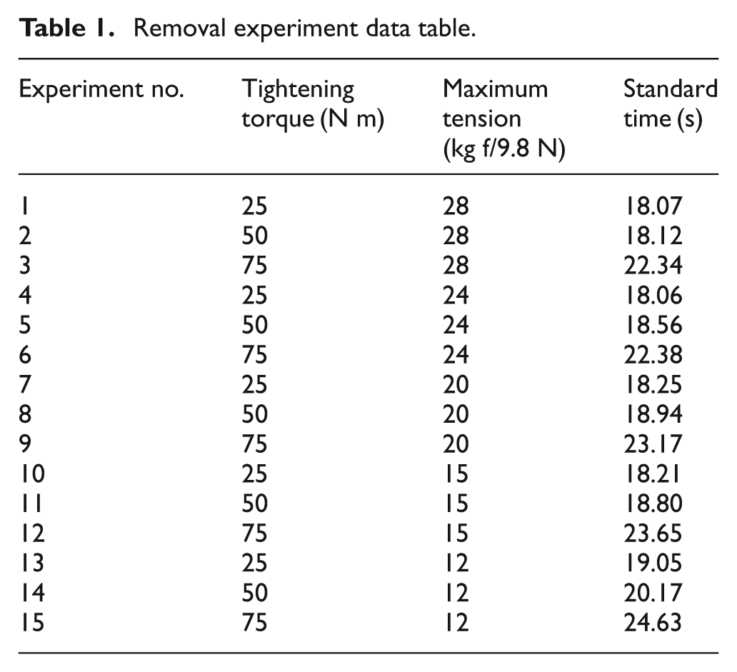
In this experiment, based on different tightening torque levels of the bolt and quality levels of operators, the corresponding 15 data points of removal standard time are obtained, as shown in Table 1. Note that at a specified corresponding level, six same bolts are removed each time and they are removed four times, that is, 24 data points of removal time of the bolt are obtained. Note that the standard time is the mean value of 24 removal time data points.
Removal experiment data table.
Influence factors ranking on component removal time based on GRA
GRA
GRA is a measurement method in grey system theory that analyses the degree of relation in a discrete sequence. In the case when experiments are ambiguous or when the experimental method cannot be carried out exactly, grey analysis helps to compensate for the shortcomings in statistical regression. 27 GRA is actually a measurement of the absolute value of the data difference between sequences, and it could be used to measure the approximate correlation between sequences.28,29
Data pre-processing
Data pre-processing is normally required since the range and unit in one data sequence may differ from the others. Data pre-processing is also necessary when the sequence scatter range is too large or when the directions of the target in the sequences are different. It is a means of transferring the original sequence to a comparable or target sequence. Depending on the characteristics of a data sequence, we have three typical methodologies of data pre-processing available for the GRA, namely, transformation method of the initial value, transformation method of the mean value and normalized transformation method.28,29 In order to calculate concisely a grey relational degree, the second method is adopted in this work.
Let a group of original sequences be
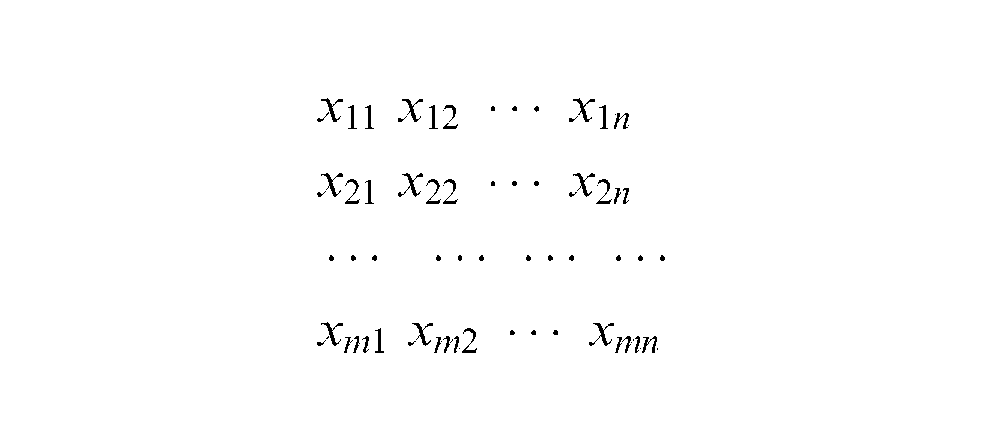
Let
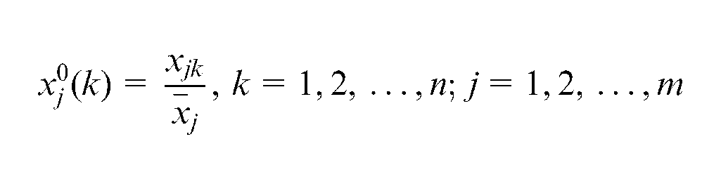
Then, a group of new comparable or target sequences is obtained, namely
The above-mentioned process is called the transformation of the mean value of data.
Grey relational coefficient and grey relational grade
In GRA, grey relational grade (degree) is defined as the extent of the relation between two sequences. Given two sequences, one can treat one as a reference sequence and another as comparison one. Let
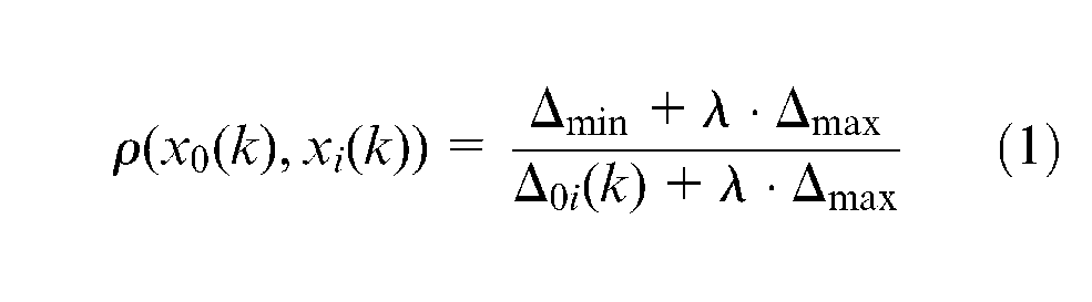
where
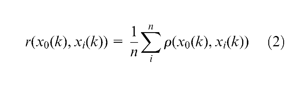
After the grey relational coefficient is derived, it is usual to take the average value of the grey relational coefficients between two sequences as the grey relational degree of ones as follows
Grey relational grade r is a value from 0 to 1, namely,
GRA-based influence factor analysis
Based on GRA and obtained experimental data shown in section ‘Removal experiment’, the influence factor analysis and the ranking of the bolt removal time can be presented in the following.
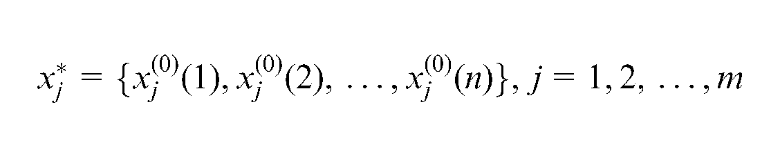
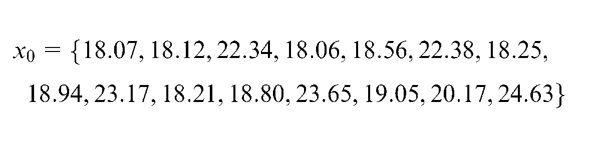
The removal time of the bolt x0 is viewed as the original reference sequence, which has 15 values,
Two factor data, namely, the tightening torque of the bolt x1 and the maximum tension of the operator x2, are seen as original comparison sequences, respectively
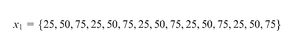
Let
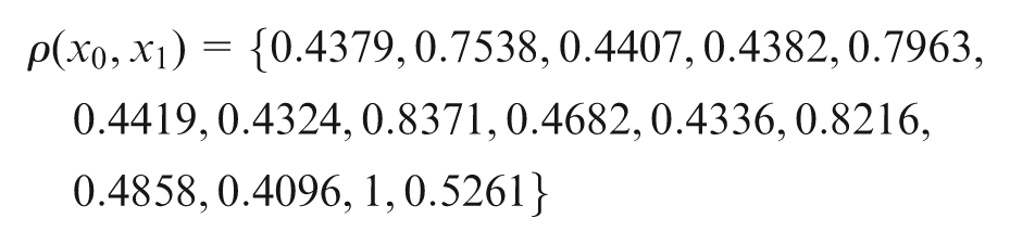
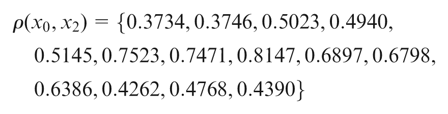
After the coefficient is averaged, the grey relational grade of the tightening torque of the bolt and the maximum tension of the operator on the removal time of the bolt are obtained, respectively


Based on the results of the grey relational grade, we can say that the influence of the tightening torque of the bolt on removal time x1 is larger than the influence the maximum tension of the operator on the removal time x2, namely, the influence factor ranking on removal time of the bolt is x1 > x2. In other words, the removal condition of a product has a significant impact on the disassembly decision-making. This result reflects the actual execution of disassembly practice.
In addition, two results of the grey relational grade are not very different, thereby indicating that the quality of the worker has an important impact on the removal time similarly. Therefore, when we discuss the prediction issue of the removal time next, both of them should be considered.
Prediction of removal time
Performing the prediction of the removal time can provide better judgment and support for disassembly decision-making and practice. Thus, based on the above-analysed two factors greatly influenced the removal time taken as the input variables in prediction and obtained removal time data regarded a comparative variable of prediction results, the prediction of removal time of the bolt is presented in the following.
In addition, considering the strong and non-linear relationship between the prediction target and its factors, we propose to use the following three methods to establish a prediction model for the removal time of the bolt, namely, multiple linear regressions (MLR), artificial neural networks (ANN) and optimized artificial neural networks based on genetic algorithm (GA-ANN) methods and their comparative results.
Prediction methods and algorithms
MLR model
MLR method was first introduced by Francis Galton in the late 19th century. Due to its good regression and prediction ability, it can be widely used to deal with such a variety of issues as biological, economic, chemical and engineering problems.30–32 In this work, it is used to predict the removal time of a component in an assembly.
An MLR model is generalized as
where t0 represents the prediction target variable or dependent variable, and
Since only two factors are considered in the example, the prediction model of removal time is expressed as

where the dependent variable t0 represents the removal time and y1 and y2 represent the tightening torque of the bolt x1 and the maximum tension of the operator x2, respectively.
Based on the above discussions, it can be seen that a dependent variable is considered as the combination of independent variables subject to their coefficients. Thus, only after their coefficients are determined can we realize effectively the prediction of the removal time. In this work, these coefficient can be obtained by the following MATLAB function, namely, regress.
ANN
ANN has been developed as generalizations of mathematical models of biological nervous systems. The basic elements of ANN are artificial neurons. In a simplified mathematical model of the neurons, the effects of synapses are represented by connection weights that modulate the effect of the associated input signals, and the non-linear characteristic exhibited by neurons is represented by a transfer function. The neuron impulse is then computed as the weighted sum of the input signals, transformed by the transfer function. The learning capability of an artificial neuron is achieved by adjusting its weights. The learning purpose in ANN is to update weights, such that given inputs, desired outputs are obtained. ANN learns the correlated patterns between input data sets and corresponding target values. After training, ANN is used to predict the outcome of independent input data or variable.33,34
In the prediction process of the removal time, we adopt a general ANN structure composed of three layers, namely, input, hidden and output layers. Its transfer function is a sigmoid function in this work.
The number of input neurons of the ANN structure is the number of input variables, namely, two influence factors; thus, the number of input neurons is 2. The number of output neurons is one representing the removal time of a component.
For the ANN structure, determining the best number of hidden neurons is one of the important problems. The number of hidden neurons can be infinite in theory but finite in practice due to two reasons: (1) Too many hidden neurons increase the training time and response time of the trained ANN and (2) too few hidden neurons make the ANN lack generalization ability. Therefore, it can usually be determined by the following formula:
In addition, learning an ANN, which is the calculation of the weights of the connections, is achieved by minimizing the error between its output and the actual output over a number of available training data points. In this article, the error term is controlled by the following MATLAB function, namely, net.trainParam.goal. It denotes the mean squared error between the output of ANN and the actual output over a number of available training data points, and it is 0.0000004 in this article.
The ANN algorithm is presented as follows:
Step 1. Initialize the number of neurons of input, hidden and output layers and initialize weighting vector w.
Step 2. Calculate the output of the hidden layer, the output of output layer and adjust the corresponding weights w.
Step 3. Calculate the error term, namely, training performance goal. If it is larger than the given error term value, go to Step 2 or otherwise end.
GA-ANN
Genetic algorithms (GA) form a class of adaptive heuristics based on principles derived from the dynamics of natural population genetics. 36 GA starts with a randomized population of parent chromosomes (numeric vectors) representing various possible solutions to a problem. The individual components (numeric values) within a chromosome are referred to as genes. New child chromosomes are generated by selection, crossover and mutation operations. All chromosomes are then evaluated according to a fitness (or objective) function, with the fittest surviving into the next generation. Generally, when the given maximum generation is reached, the algorithm ends. The best chromosome is assigned to the optimal solution of the problem. 37 In this article, we propose to use GA to optimize weights and thresholds of neural networks (NN) to improve its performance. Its steps are presented as follows:
Step 1. Initialize
Step 2. Determine the fitness or evaluation function. Based on a chromosome obtained by Step 1, weights and thresholds of the NN are assigned. If specified training data are input, forecast output of the trained NN can be obtained. In this article, the inversed function of the sum of absolute difference between forecast outputs of the trained NN and actual outputs is considered as the fitness value
where
Step 3. A selection operation is implemented by pinning the roulette wheel method. That is, a selection strategy is executed according to the fitness value. Thus, the selection probability

Step 4. A crossover operation is implemented by a real number crossover method. The operation in position
where
Step 5. A mutation operation is implemented as follows: given the jth gene
where
Step 6. Weights and thresholds of the NN are assigned based on the optimal chromosome from GA, and the optimal forecast outputs of the trained NN are obtained based on the obtained best weights and thresholds.
When it is used to predict the removal time, the following parameters are adopted. The number of input and output neurons of ANN is set to be
Prediction and performance evaluation
Based on the above-described algorithm, the prediction and its results on removal time of the bolt are presented in this section.
Prediction of removal time
Predicted result of MLR
Initializing the input data of MLR, namely, 15 experimental data of tightening torque of the bolt and maximum tension of the operator, combined with the experiment data of the removal time, related coefficients of MLR models is obtained by the MATLAB function regress. If they are brought into equation (4), then the MLR model for prediction of removal time of the bolt is obtained as follows
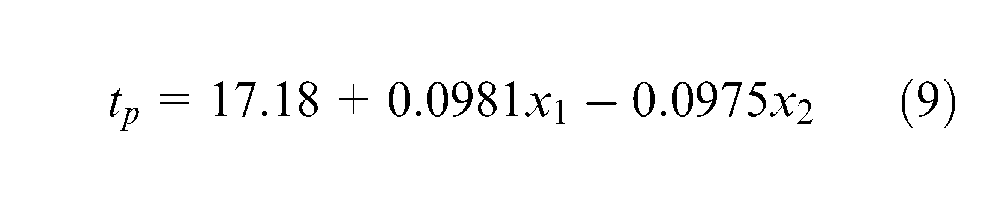
Based on the determined MLR model, combined with two factor data, the predicted value of removal time is obtained, as listed in the third column of Table 2.
Prediction results of MLR, ANN and GA-ANN models.
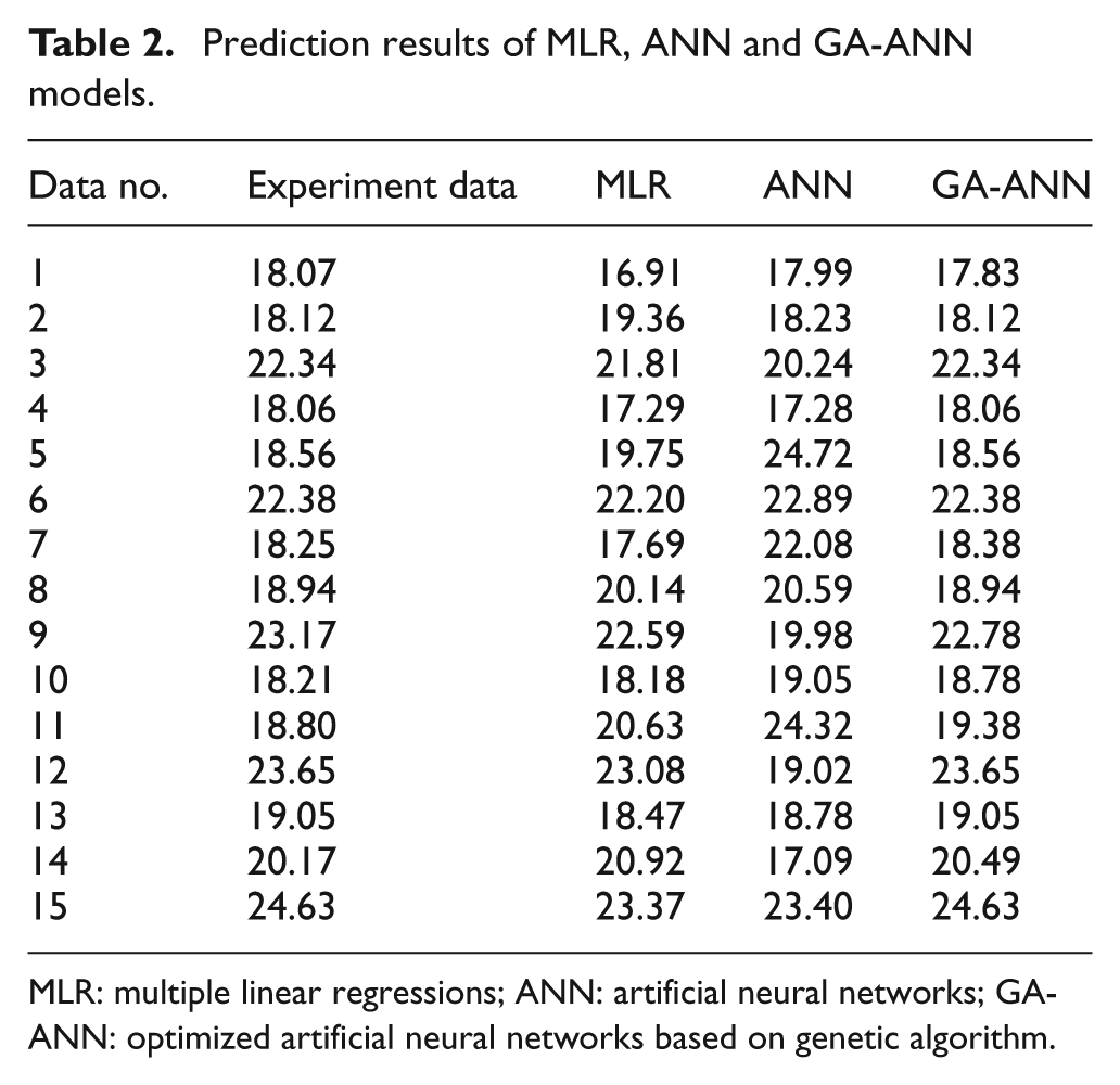
MLR: multiple linear regressions; ANN: artificial neural networks; GA-ANN: optimized artificial neural networks based on genetic algorithm.
Predicted result of ANN
Take two factors and removal time as input and output data of ANN training, respectively. After the ANN algorithm is run, the specific ANN is established. Then two factors x1 and x2 are brought into the trained ANN to obtain the predicted result of removal time, as listed in the fourth column of Table 2.
Predicted result of GA-ANN
Similarly, take two factors and removal time as input and output of GA-ANN training, respectively. After the ANN algorithm is run, the specific GA-ANN is established. Then two factors x1 and x2 are brought into the trained GA-ANN to obtain the predicted result of removal time, as listed in the last column of Table 2.
Prediction performance evaluation
In order to quantitatively evaluate the performance of three prediction models, the following evaluation parameters are introduced: the mean value of absolute error (MV), standard deviation of absolute error (SD) and correlation coefficient (
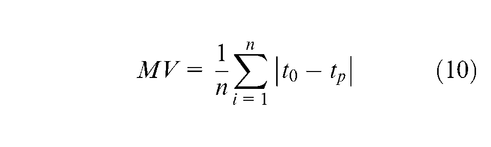
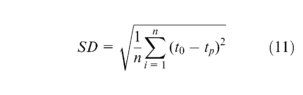
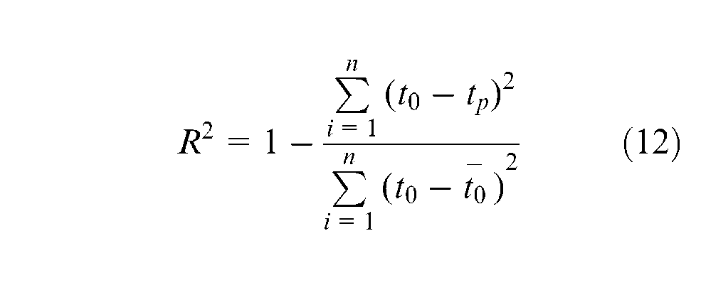
where
In addition, practical implications of these three parameters are described as follows:
Based on the presented performance parameters, their results are calculated and shown in Table 3. From Table 3, the following conclusions can be obtained: first, for these prediction models, their correlation coefficient (
Performance comparison for different prediction models.
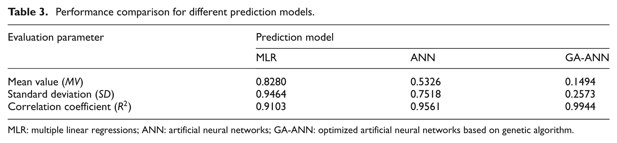
MLR: multiple linear regressions; ANN: artificial neural networks; GA-ANN: optimized artificial neural networks based on genetic algorithm.
Conclusion
Influence factor analysis and accurate prediction on product disassembly time play an important role in a product recovery management system. In order to determine the main factors of product disassembly and perform prediction on product disassembly time, this work takes the bolt as a removal object, and designs its removal experiment considering some factors influencing a removal process. Second, this work introduces a GRA method to solve the ranking issue of removal factors for the first time. Finally, based on the analysed and obtained main factors, this work establishes the following three prediction models on removal time: MLR, ANN and GA-ANN models. The results reveal that they are feasible and accurate when used to predict the component removal time. The obtained results can be used to guide decision-makers in making better disassembly decisions.
There exist some limitations with the proposed method. The future work is to design disassembly experiments considering more factors (e.g. the characteristic parameters of the removal part and the types of removal tools) to provide the best decision support of disassembly practice. In addition, the application of the research results to more complex product disassembly needs to be explored.
Footnotes
Acknowledgements
We would like to thank the editor and reviewers for the insightful comments that helped us improve this article. In addition, we would like to thank Prof. M. C. Zhou for his valuable comments to improve the presentation of this article.
Declaration of conflicting interests
The authors declare that there is no conflict of interest.
Funding
This work is financially supported by the Fundamental Research Funds for the Central Universities of China (DL12BB32), Natural Science Foundation of China under grant no. 61203037 and New Century Excellent Talents in University under grant no. NCET-12-0921.