Using Taguchi method to optimise performance and product cost at the conceptual stage of design

Abstract

The difficulty of obtaining a useful cost estimate at the design stage has long been acknowledged. Data for new products are hardly available and product specifications are often expressed as a range of values; yet, only limited progress has been made to date to improve the quality of the average cost estimate at the conceptual design stage. The aim of this research is to improve the quality of the cost estimate (average cost) at the conceptual stage of design to assist designers to consider cost as a critical factor in selecting the most appropriate design concept. This research investigates the use of Taguchi’s orthogonal array approach to reduce the variation in the product specification (when expressed as a range of values) in order to improve the quality of the average estimated cost for each concept at the conceptual stage of design. A new process has been created, and to validate the process, an industrial case study has been undertaken.

Introduction

One of the most difficult tasks undertaken by designers is to evaluate the cost of a future design. When designers start to design a new product, cost is a critical factor in determining whether the product will be produced or not. The cost of the product in the market place is one of the key contributions to success. ¹

To ensure the product price is appropriate, the cost estimate should be available as early in the design process as possible in order to provide valuable information to product designers. However, existing techniques are prone to error because the mistakes in cost estimating are many and varied. An example is the Scottish Parliament construction project. The project increased in cost 10-fold to £431m instead of the £40m predicted. ² Increasing the costs for the 2012 Olympics from £3.4b to £9.3b is another example. ³ The makers of the Airbus A380 aircraft offer another high-profile example where the actual costs differ from those predicted. ⁴ The F/A-22 aircraft has also experienced significant cost growth from its original estimated programme cost. ⁵ Higher than predicted project costs in the construction industry are not unusual since, current tendering processes force suppliers to tie down on costs to 98%. ⁶ Flyvbjerg et al. ⁷ indicate that over the past 70 years, cost underestimation has not decreased. They found that not only 90% of transportation projects were underestimated but also the actual costs for rail and road projects were on average 45% and 20% higher than estimated costs, respectively. They concluded that for all types of projects, estimated costs were lower than the actual cost by 28%. Many authors^8–11 indicate that both underestimates and overestimates can have negative impacts on a company’s business. Asiedu and Gu ¹² state that

• ‘The greater the underestimate, the greater the actual expenditure’.

• ‘The greater the overestimate the greater the actual expenditure’.

• ‘The most realistic estimate results in the most economical project cost’.

All these illustrate why cost estimation at the early design stages is very important for companies.

Many authors^13–16 have pointed out the importance of cost estimation at the design stage. Corbett ¹³ indicates that 80% of a product cost is committed during the early design stage. Mileham et al., ¹⁷ Dowlatshahi ¹⁶ and Hundal ¹⁸ agree that 70%–80% of a product cost is determined during the early design stage. As previously stated, Figure 1 depicts ¹⁵ the importance of cost estimation at the design stage and the cost commitment curve. This figure illustrates how decrease at the early design stage commits 80% of the product cost. Estimating cost accurately at this stage can help the designers and estimators to improve product designs in terms of performance and cost. ¹⁹

Figure 1.

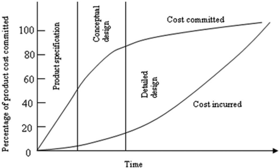
Cost commitment during design. ¹⁵

Although designers understand the importance of cost estimation at the conceptual stage of design, in general, cost estimation is usually very limited or does not really happen as the information is sparse and designers tend to wait until more detail and information is available.

Conceptual design (design development process) and available information at this stage

The previous section explained the importance of cost estimation at the conceptual stage of design and how available information can be limited at this stage. This section explains the definition of the conceptual stage of design used in this research and the available information for designers to estimate the cost.

Cross ²⁰ explains 50 years of design history and illustrates new design consists of scientific methods. There are many different definitions of design, each referring to a special application. Raymer ²¹ describes how the analytical processes are important in design especially for manufacturers to meet requirements. Design is a non-unique iterative process, the aim of which is to reach the best comprise for a number of conflicting requirements. Whether the need is for a totally new item or for the development of an existing product the design procedure commences with an interpretation of the requirements into a first concept. ²² Cross ²³ defines design as a set of activities from the establishment of a product requirement specification to the generation of the information necessary for making the product. Crossland ²⁴ and Mistree et al. ²⁵ provide a comprehensive review of developments in the field of design theories and methodologies. Although there are different definitions of design, in the majority of cases, it is defined as providing a new solution to a problem and can be broken into the three major stages: ²¹

1. Conceptual design;

2. Embodiment design;

3. Detail design.

Conceptual design, where is the focus of this research, is considered to be the most important stage in terms of decision-making in design. It is during the conceptual design phase that the basic questions of configuration arrangement, size, weight and performance are answered. ²¹ In the embodiment and detail design stages, material specifications, dimensions, surface condition and tolerances are specified in the fullest possible detail for manufacturing.

The concept stage varies from industry to industry and product to product. Ullman ¹⁵ introduces three major steps for conceptual design: generating concepts, evaluating concepts and selecting concepts. Figure 2, adapted from Pahl et al., ²⁶ illustrates an alternative view that conceptual design can be broken down into four major steps:

1. Abstracting to identify the essential problems;

2. Establishing function structures;

3. Developing working structures;

4. Developing concepts.

Figure 2.

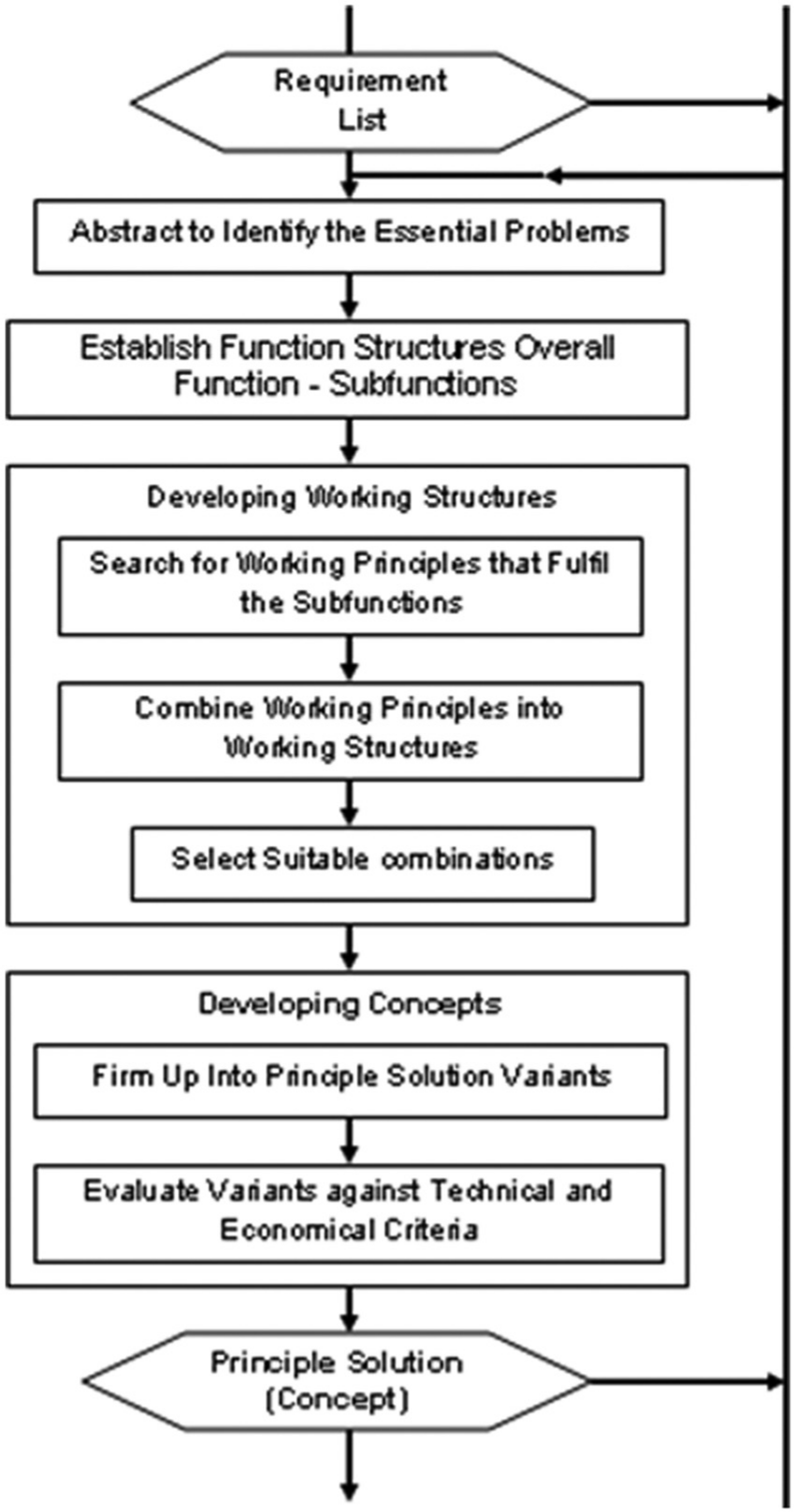
Steps of conceptual design. ²⁶

Abstracting to identify the essential problem stage is about formulating the problem. After identifying the problem, designers establish function structures, then they develop working structures and finally different concepts are created and the most appropriate one is selected.

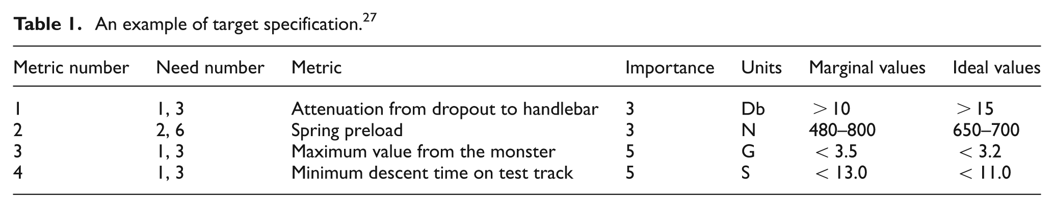
Ulrich and Eppinger ²⁷ created a generic diagram (Figure 3), which shows the activities that must be considered for all projects. These activities are identify customer needs, set target specification (ideal customer requirements set as design target), generate product concepts, select product concepts, test product concepts and set final specification. Often designers do not consider the identify customer needs stage, as part of the concept development process. Ulrich, however, emphasises the importance of this stage before the concept development process begins. The next stage is setting the target specification that is normally considered as the first stage in the concept development process. At the target specification stage, agreement on the general design functions is achieved. The target specifications are set to meet the design requirements. However, they are established before the designers know what constraints the product technology will place on the design and what can be achieved. ²⁷ Hence, targets are typically expressed as a range of values, shown in Table 1. For the target specification, the values are typically wide and are reduced in the final specification list. It is important to note that the target specification mentioned throughout this article is also known as customer requirements, that is, specifying what the customer would like.

Table 1.

An example of target specification. ²⁷

Metric number	Need number	Metric	Importance	Units	Marginal values	Ideal values
1	1, 3	Attenuation from dropout to handlebar	3	Db	>10	>15
2	2, 6	Spring preload	3	N	480–800	650–700
3	1, 3	Maximum value from the monster	5	G	<3.5	<3.2
4	1, 3	Minimum descent time on test track	5	S	<13.0	<11.0

Figure 3.

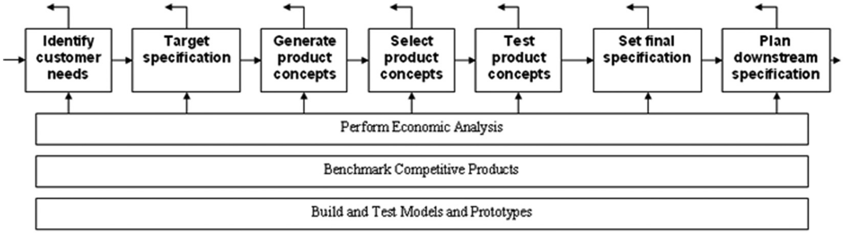
Concept development process. ²⁷

As shown in Figure 3, after the target specification stage, the next stage is to generate product concepts. Designers describe the technology, form and working principles of a product in this stage. Also in this stage, designers generate many concepts from which just a few will be selected. Designers then reduce the number of concepts to typically two or more when selecting product concept. ²⁷

As described, designers create a product target specification (Table 1) before starting to generate concepts. Therefore, the targets (metrics) are typically expressed as a range of values (Table 1). Designers’ rate metrics in terms of their functionality or performance using, for example, quality function deployment (QFD) techniques (which are described in detail in Shillito ²⁸ ), and a rating example is shown in the importance column in Table 1. The focus of the research for this article is based on rating these metrics in terms of cost as well as performance in order to carry out a more informed optimisation between performance and cost. It is important to note that, since the target specification is typically the only available information at the beginning of the conceptual stage of design, this stage is the main focus of this research.

Research hypothesis

As up to 80% of a product cost is committed at the conceptual stage of design, the research question is thus how can we improve the quality of the average cost during the early design stages using the limited information available? To answer this question, a novel process is introduced in this article.

As previously stated at the conceptual stage of design, data are often limited, and estimating cost accurately at this stage is very difficult. This is exacerbated for new products when product specifications (target specification) are expressed in ranges (see Table 1). In order to improve the quality of the average cost (the lower variation or variance) at the target specification stage, a new method proposed to rate the metrics in the target specification (Table 1) in terms of cost. Designers then put the cost and performance ratings together (performance rating is shown in Table 1) in order to carry out an informed optimisation between performance and cost to estimate the lowest possible average cost with the lowest possible variance for each concept (while meeting the product specification).

As the aim of the research presented in this article was to improve the quality of the cost estimate, the hypothesis was to use traditional quality improvement techniques within cost estimation. Various techniques were reviewed. These include QFD, ²⁹ failure mode and effect analysis (FMEA) ²⁹ and traditional design of experiments and Taguchi method. ³⁰ From a review of these techniques, Taguchi’s orthogonal array approach was selected as it offered the opportunity to reduce the variance in the average cost. Previous research has shown that how the Taguchi method has been used to improve the quality characteristics of products;^31–34 this article does not focus on improving the quality of the product; however, the aim was to utilise these techniques to improve the quality of the average cost. Quality in this article is defined as reducing the variance in the cost estimate while optimising the product specification.

Proposed solution

The new methodology uses Taguchi’s orthogonal array approach to assess and identify input values and their impact on a product’s average cost. For the analysis, SEER-DFM (SEER- Design for Manufacture) ³⁵ was used to estimate the manufacturing cost, and an industrial case study was undertaken to establish the viability of the new process.

In summary, to improve the quality of cost estimates, the following specific objectives were identified:

• To rate the metrics in the product specification and identify metrics that have the greatest impact on the average cost (rating metrics in terms of cost);

• To analyse the effect of different levels and carry out optimisation between performance and cost;

• To estimate the lowest possible average cost with the lowest possible variation by reducing the variation in the product specification while maximising performance.

Figure 4 illustrates a typical design process. The dashed box illustrates the focus of the research presented in this article.

Figure 4.

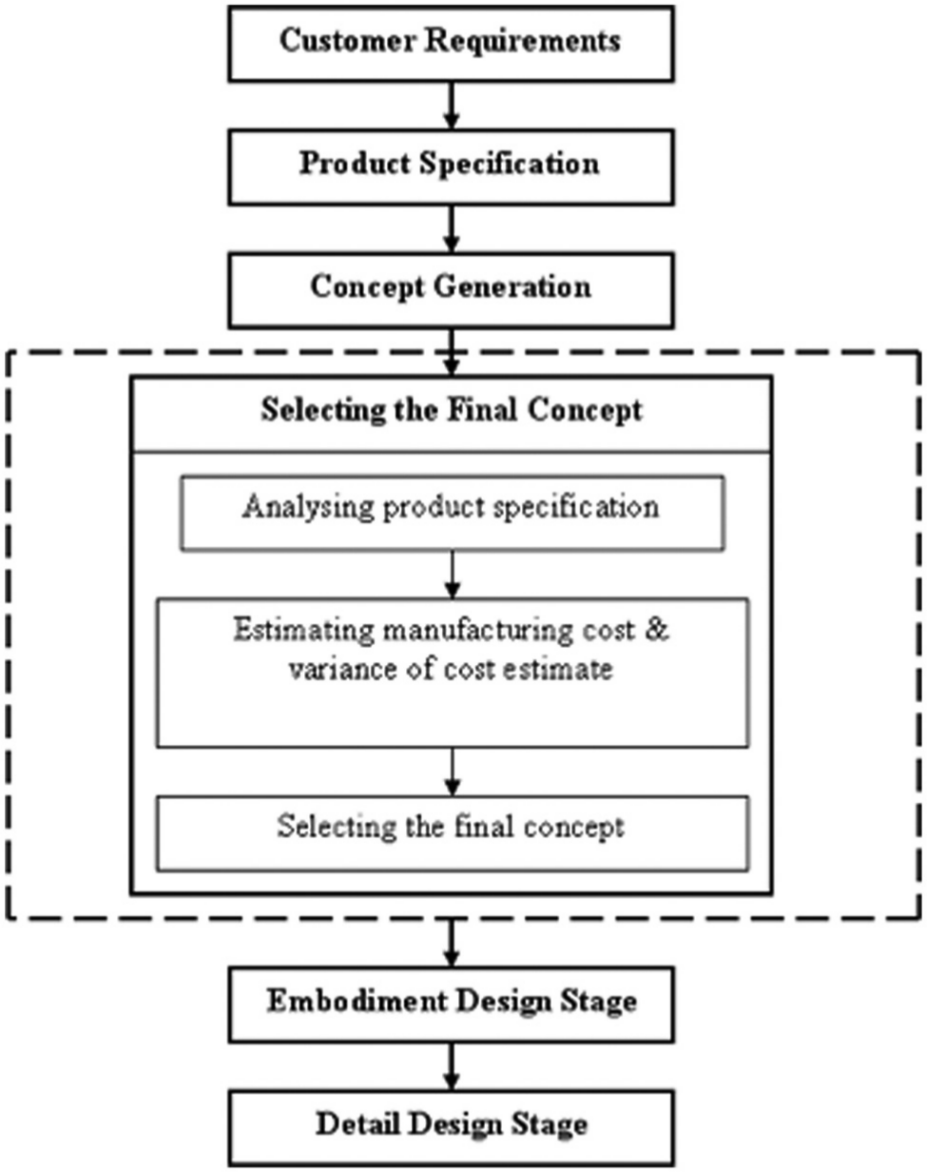
Design process and focus of the research presented in this article.

Proposed process for estimating product cost at the conceptual stage of design

Figure 5 shows the three phases of the new methodology and its applicability at the concept design stage of a product. The three phases within the process include analysing the product specification, estimating the manufacturing cost and variance of the cost estimate and selecting the final concept. Each of these phases is described in detail in the next sections via an applied case study.

Figure 5.

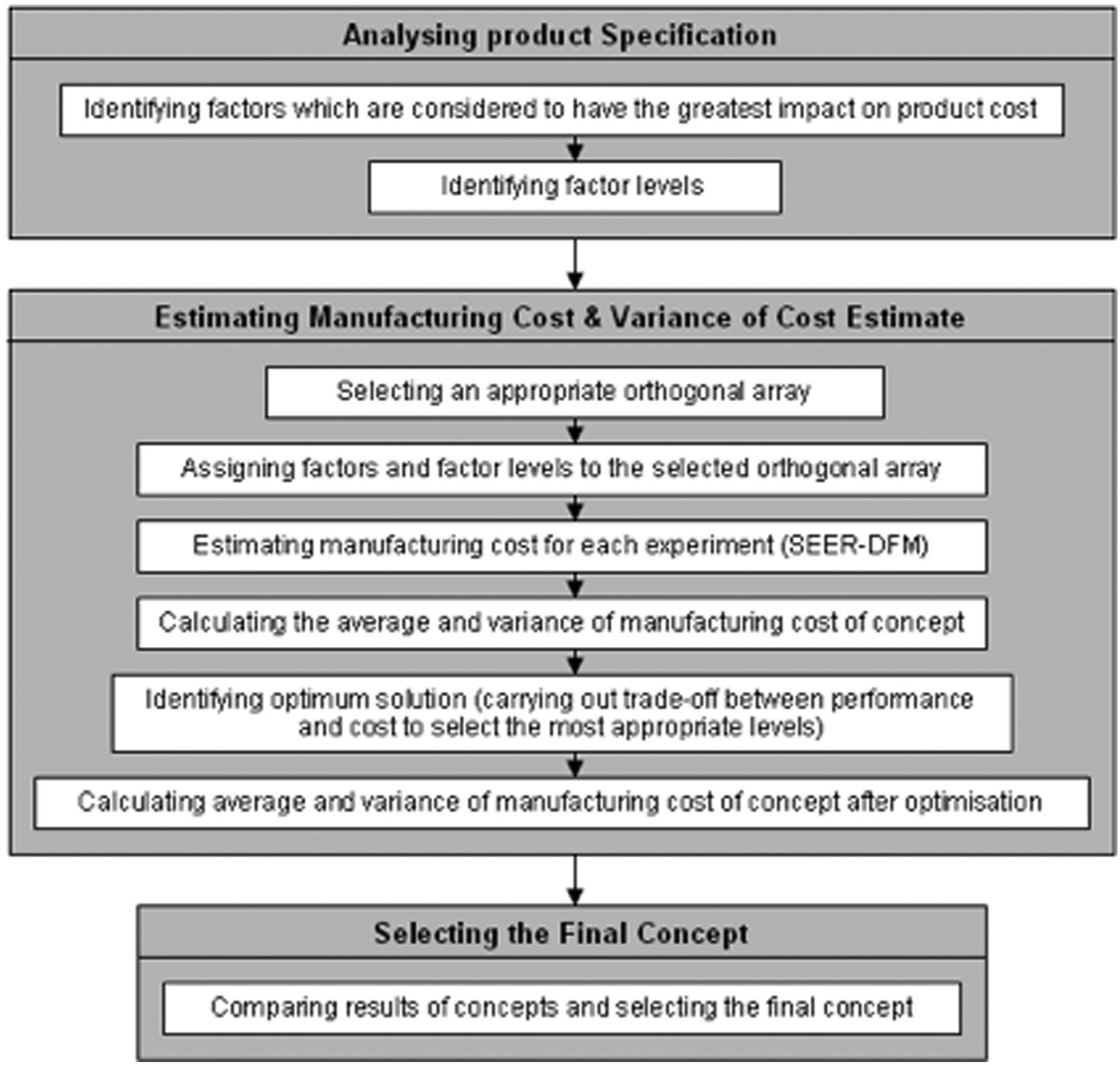
Specification/cost trade-off process.

Two main tools are used in the process. First, Taguchi’s orthogonal array approach is used to identify factors and assign these factors to the appropriate orthogonal array. Second, a cost estimating tool is used. In this research, SEER-DFM ³⁵ is used to estimate the average cost for each concept, although other cost estimating tools are also appropriate. Each of these should be implemented separately as part of the new process in order to estimate the concept’s lowest possible average cost (manufacturing cost) with the lowest possible variation. Section 5 of the article presents the new process via a step-by-step industrial-based case study.

Case study

This section describes the implementation of the new process (shown in Figure 5) for a real industrial case study undertaken with DePuy International. ³⁶ All three phases of the new process are explained in detail, and the outcomes discussed. Due to confidentiality reasons, full details of the designs, components and volumes of the designs are not provided.

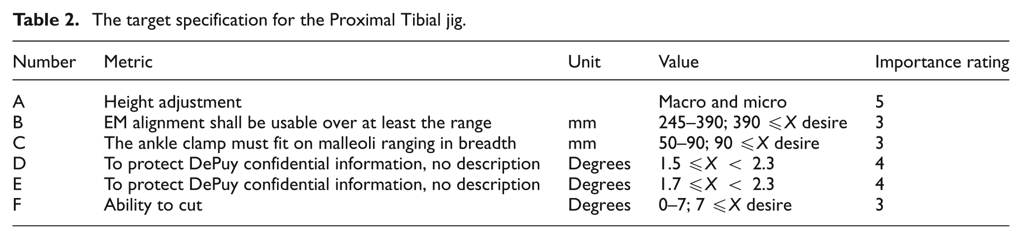
The aim of the case study was to design a new Proximal Tibial Jig in order to assist surgeons to cut the Tibial bone in the knee easily and accurately during knee replacement operations. The design activity was undertaken by designers within DePuy. The user requirements were identified and then translated into engineering terms and a target specification created as summarised in Table 2. From the requirements, six metrics or factors (A, B, C, D, E and F) were identified, and these factors were expressed as a range of values. The factors in the target specification were rated in terms of their functionality using the QFD technique, that is the importance rating depicted in the final column of Table 2.

Table 2.

The target specification for the Proximal Tibial jig

Number	Metric	Unit	Value	Importance rating
A	Height adjustment		Macro and micro	5
B	EM alignment shall be usable over at least the range	mm	245–390; 390 ≤X desire	3
C	The ankle clamp must fit on malleoli ranging in breadth	mm	50–90; 90 ≤X desire	3
D	To protect DePuy confidential information, no description	Degrees	1.5 ≤X < 2.3	4
E	To protect DePuy confidential information, no description	Degrees	1.7 ≤X < 2.3	4
F	Ability to cut	Degrees	0–7; 7 ≤X desire	3

Using the defined target specification, six concept designs were created.

• Concept 01 (All Dial Rack Based, Live Spring).

• Concept 02 (Combo A Dials and Levers, Live Spring).

• Concept 03 (All Pinch Rack Based, Constant Spring).

• Concept 04 (All Dial Helical Based, Constant Spring).

• Concept 05 (All Pinch Rack Based, Real-Feel).

• Concept 06 (All Dial Helical Based, Real-Feel).

As mentioned in the previous section, the aim of this research was to estimate the lowest possible average cost and the lowest possible variance of the average cost that the designers in DePuy could achieve by changing the factor values (shown in Table 2) in the design (while meeting the specifications). This was achieved by applying the process (Figure 5) to rate the factors (A, B, C, D, E and F, Table 2) in terms of cost and then carrying out the trade-off between performance and cost at the conceptual stage of design.

Based on the specification/cost trade-off process, the following sections illustrate the step-by-step implementation of the new process for each concept in the Proximal Tibial jig project (agreed production quantities on which to base the cost information were provided by DePuy, but for confidentiality reasons, they have not been published here).

Concept 01

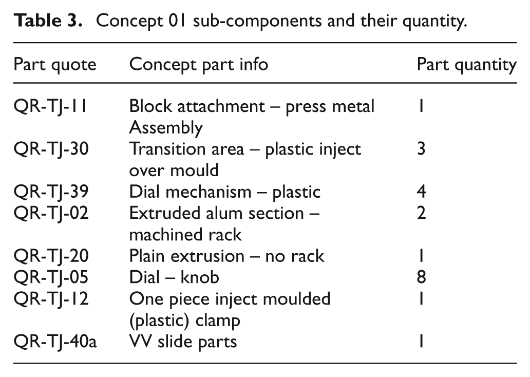
Figure 6 illustrates the computer-aided design (CAD) model of concept 01. The general shape of other concepts is the same as concept 01 but with different sub-components. Table 3 shows the sub-components and parts used in concept 01 and their quantity. Because of product confidentiality, information about each part cannot be shown here. (It is important to note that the case study in this article has relative small number of well-designed components. The new process proposed in this article can also be used for products with high complexity, with thousand of sub-components. This will be explained in the following sections.)

Table 3.

Concept 01 sub-components and their quantity

Part quote	Concept part info	Part quantity
QR-TJ-11	Block attachment – press metal Assembly	1
QR-TJ-30	Transition area – plastic inject over mould	3
QR-TJ-39	Dial mechanism – plastic	4
QR-TJ-02	Extruded alum section – machined rack	2
QR-TJ-20	Plain extrusion – no rack	1
QR-TJ-05	Dial – knob	8
QR-TJ-12	One piece inject moulded (plastic) clamp	1
QR-TJ-40a	VV slide parts	1

Figure 6.

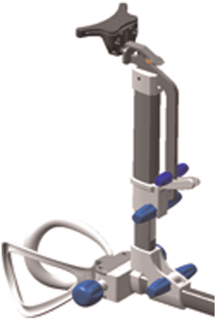
Concept 01.

To estimate the lowest possible manufacturing cost with the lowest possible variance for concept 01, the three phases (analysing product specification, estimating manufacturing cost and variance of cost estimate and selecting the most appropriate concept), shown in Figure 5, were then followed.

Phase 1 – analysing product specification

Identifying factors that are thought to have the greatest impact on product cost

The first stage was to identify special factors, which were thought to have the greatest impact on the cost of concept 01. For products with few factors (normally less than 10 factors), there is no need to identify special factors as all the factors can be assessed economically. Since only six factors (A, B, C, D, E and F, Table 4) had to be considered for the Proximal Tibial Jig, all these factors were assessed. Based on the analysis, it was also decided to ascertain whether the interaction between factors A and B could be considered as a separate factor A × B (this means interaction between factors A and B). In this example, the number of factors is less than 10, so all the factors can be considered. If the same technique was to be used for products with greater than 10 factors, designers have two options. First, all the factors can be modelled; however, the authors’ view in this would be time consuming. The second option is to use the Delphi method to identify factors, which are perceived to have the highest impact on product costs. This will enable a more focussed view and act as a guide in determining which factors to prioritise in the initial stages. Details of how designers can use the Delphi technique to identify factors with higher impact on the product costs can be found in Saravi et al. ³⁷

Table 4.

Factor levels.

Number	Metric	Value	Levels	Importance rating
A	Height adjustment	Macro and micro	Level 1: macro; level 2: micro	5
B	EM alignment shall be usable over at least the range	245–390; 390 ≤X desire	Level 1: 390; level 2: 400	3
C	The ankle clamp must fit on malleoli ranging in breadth	50–90; 90 ≤X desire	Level 1: 90; level 2: 100	3
D	To protect DePuy confidential information, no description	1.5 ≤X < 2.3	Level 1: 1.5; level 2: 2.0	4
E	To protect DePuy confidential information, no description	1.7 ≤X < 2.3	Level 1: 1.7; level 2: 2.0	4
F	Ability to cut	0–7; 7 ≤X desire	Level 1: 7; level 2: 10	3
A × B	Interaction between factors A and B		Level 1: A × B1; level 2: A × B2

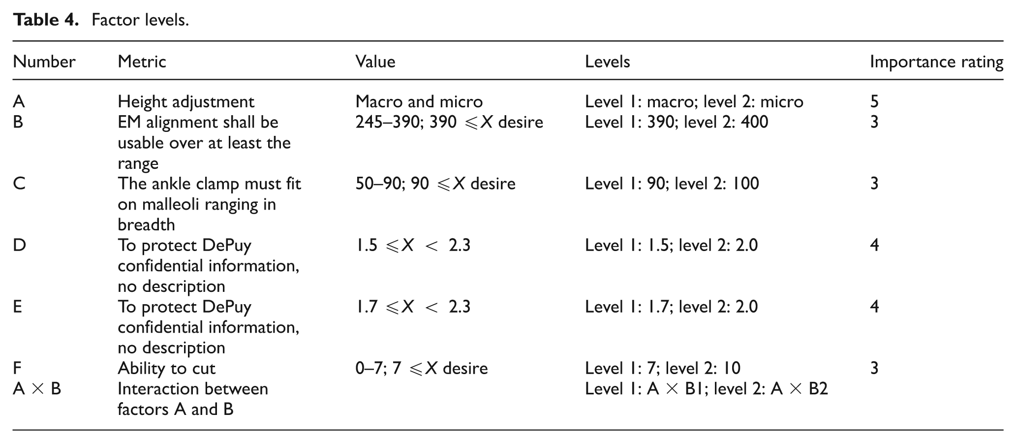
Identifying factor levels

The number of factor levels dictates the number of experiments required. Details on how to identify factor levels can be found in Belavendram. ³⁰ Levels identified for each factor were added to Table 4. In this example, two levels were identified for each factor.

• Factor A: Since there were two values for factor A, level 1 (A1) was macro and level 2 (A2) was micro.

• Factor B: As the product specification indicated that the new product should at a minimum covers the range 245–390 mm, and anything greater than 390 mm (390 ≤X) was a desire; level 1 (B1) was 390 mm and level 2 (B2) was 400 mm. These values were selected based on discussions with the design experts who highlighted the advantages of achieving greater than 390 mm.

• Factor C: The new product should cover the range 50–90 mm, and anything greater than 90 mm is a desire. Therefore, level 1 (C1) was 90 mm and level 2 (C2) was 100 mm.

• Factor D: As the value for factor D was 1.5°≤X < 2.3°, level 1 (D1) was 1.5° and level 2 (D2) was 2.0°. (2.00° was selected for level 2 since the value should be between 1.5° and 2.3°. It could be any value between this range, and it was just to check the effect of the value on the product cost. More than two levels could be selected if needed.)

• Factor E: Since the value for factor E was 1.7°≤X < 2.3°, level 1 (E1) was 1.7° and level 2 (E2) was 2.0°. (2.0° was selected for level 2 since it could be any value between 1.7° and 2.3°.)

• Factor F: The new product should cover the range 0°–7°, and anything greater than 7° was a desire. Therefore level 1 (F1) was 7° and level 2 (F2) was 10°.

The ranges, levels and importance ratings were set in conjunction with design requirements for DePuy and are shown in Table 4.

Phase 2 – estimating manufacturing cost and variance of cost estimate

Selecting an appropriate orthogonal array

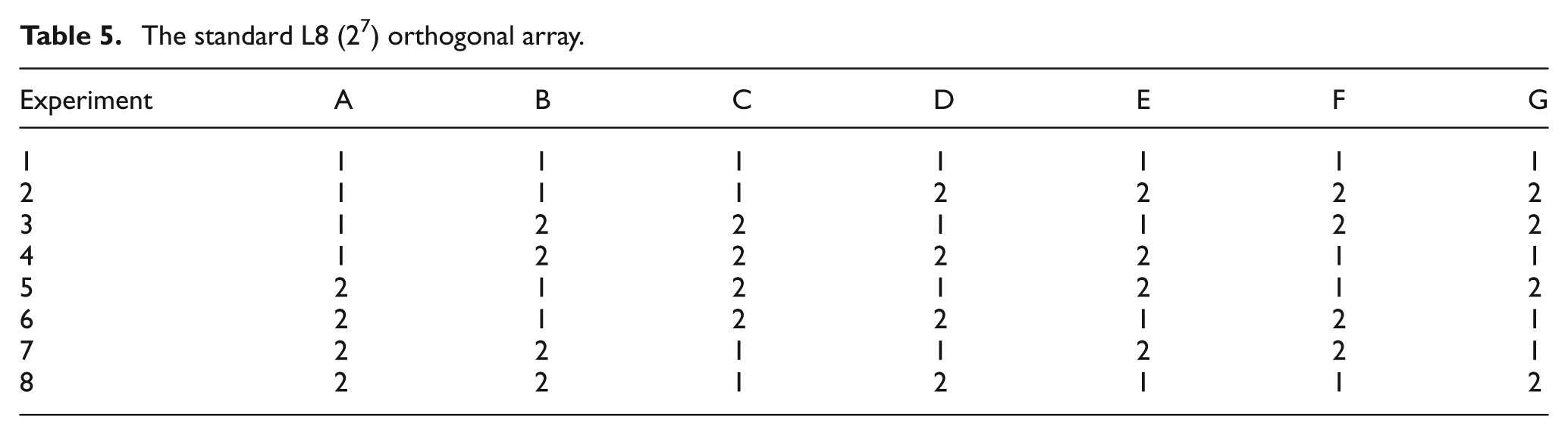
The first stage in phase 2 was to select the most appropriate orthogonal array and assign factor levels to it. As described in the previous section, six factors (A, B, C, D, E and F) and one interaction (A × B) were examined. Therefore, the smallest orthogonal array that could be used was an L8 (2⁷). Table 5 shows the standard L8 (2⁷) orthogonal array suggested by Taguchi. For products with a higher number of factors the appropriate standard orthogonal array table should be selected. In other words, it is not important how many factors designers need to consider; the most important thing is to select the right orthogonal array for the selected factors.

Table 5.

The standard L8 (2⁷) orthogonal array.

Experiment	A	B	C	D	E	F	G
1	1	1	1	1	1	1	1
2	1	1	1	2	2	2	2
3	1	2	2	1	1	2	2
4	1	2	2	2	2	1	1
5	2	1	2	1	2	1	2
6	2	1	2	2	1	2	1
7	2	2	1	1	2	2	1
8	2	2	1	2	1	1	2

Assigning factors and factor levels to the selected orthogonal array

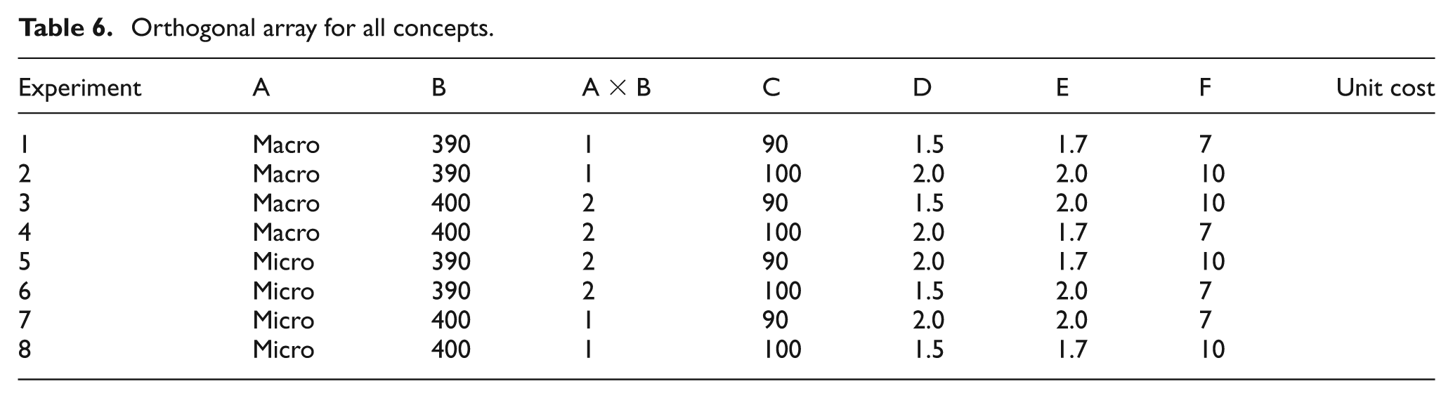
To assign factors (A, B, C, D, E, F and A × B), the linear graph (shown in Figure 7) was used. Using Figure 7 and Table 5, factors were assigned to the L8 (2⁷) orthogonal array. This is shown in Table 6.

Table 6.

Orthogonal array for all concepts

Experiment	A	B	A × B	C	D	E	F	Unit cost
1	Macro	390	1	90	1.5	1.7	7
2	Macro	390	1	100	2.0	2.0	10
3	Macro	400	2	90	1.5	2.0	10
4	Macro	400	2	100	2.0	1.7	7
5	Micro	390	2	90	2.0	1.7	10
6	Micro	390	2	100	1.5	2.0	7
7	Micro	400	1	90	2.0	2.0	7
8	Micro	400	1	100	1.5	1.7	10

Figure 7.

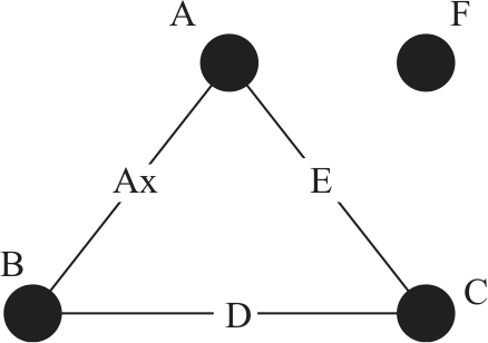
Linear graph for concept 01.

After assigning the factors, the next stage was to assign factor levels (shown in Table 6). Since experiments 1–4 (Table 5) should be at level 1, level 1 of factor A, macro was assigned to experiments 1–4. Also as experiments 5–8 (Table 5) should be at level 2, level 2 for factor A, micro was assigned to experiments 5–8. Appropriate levels were similarly added for the other factors following Table 6, that is, entering the values for each factor in terms of level 1 and level 2. Table 6 shows the average after the factors and levels have been determined. This table was the same for all six concepts and only became concept specific when the unit or manufacturing cost was added. How the manufacturing cost was calculated is explained in the following section.

Estimating manufacturing cost for each experiment (SEER-DFM)

Using Table 6, eight experiments were carried out, and the manufacturing cost for concept 01 for each experiment was estimated using the SEER-DFM software and then placed in the last column of Table 6. Although SEER-DFM is used to estimate the manufacturing cost, this process can be followed for any suitable cost estimation package, whether it is an in-house spreadsheet or another commercial package. The aim of the proposed process is to use the available information to estimate the manufacturing cost; therefore, designers can use the available information and use any appropriate cost estimation techniques to estimate the cost of the product, which enable a relative comparison between the concepts.

Table 7 shows the L8 (2⁷) orthogonal array for concept 01 after adding the estimated cost for each experiment. For example, for experiment 1, the estimated cost of concept 01 was 328.74 cost units (to protect DePuy’s confidential information, costing information has been referred to as ‘units’, which are sensitive enough to demonstrate the technique described in this article, but do not represent the true product manufacturing costs to DePuy) for the combination of factors fixed. In other words, for design concept 01 (Figure 6), if factor A was macro, factor B was 390 mm, factor C was 90 mm, factor D was 1.5°, factor E was 1.7° and factor F was 7°, the manufacturing cost of concept 01 was 328.74 cost units. The cost of the other experiments was calculated in a similar way. (It is important to note although the case study in this article has relative small number of well-designed components, the proposed process can be used for complex products as well. The most important thing is to consider all the different values for each factor and analyse the effect of changing these values on product designs.)

Table 7.

Orthogonal array and unit cost for concept 01.

Experiment	A	B	A × B	C	D	E	F	Unit cost
1	Macro	390	1	90	1.5	1.7	7	328.74
2	Macro	390	1	100	2.0	2.0	10	300.31
3	Macro	400	2	90	1.5	2.0	10	323.65
4	Macro	400	2	100	2.0	1.7	7	328.49
5	Micro	390	2	90	2.0	1.7	10	336.08
6	Micro	390	2	100	1.5	2.0	7	331.13
7	Micro	400	1	90	2.0	2.0	7	335.03
8	Micro	400	1	100	1.5	1.7	10	363.65

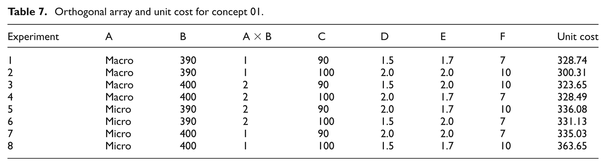
Table 7 shows that the lowest cost was 300.31 cost units and the highest cost was 363.65 cost units. This means that the lowest manufacturing cost for concept 01 was 300.31 cost units with factor A at macro, factor B 390 mm, factor C 100 mm, factor D 2.0°, factor E 2.0° and factor F 10°. The next stage calculates the variance in costs.

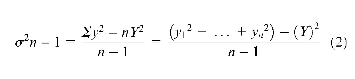
Calculating the average and variance of manufacturing cost of concept

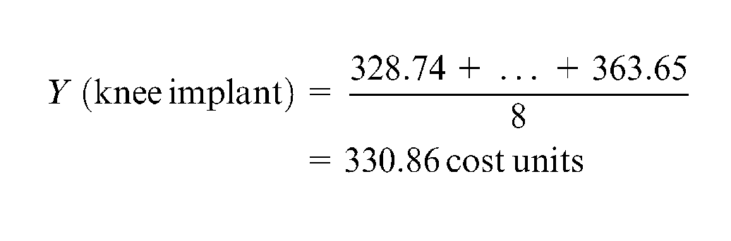
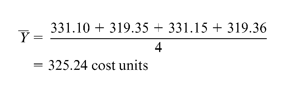
At this stage, the average manufacturing cost (equation (1)) and variance of the manufacturing cost (equation (2)) of concept 01 was calculated by averaging the unit cost of experiments 1–8 (this is called average manufacturing cost before optimisation).

The average manufacturing cost for concept 01 was

$$Y=\frac{y_1+y_2+\dots +y_n}{n}$$

(1)

where

y₁ is cost of experiment 1

y_n is cost of experiment n

n is number of experiments

Therefore, from equation (1)

$$\begin{array}{cc}\multicolumn{1}{c}{Y\left(\text{knee}\text{implant}\right)}& =\frac{328.74+\dots +363.65}{8}\hfill \\ \hfill =330.86\text{cost}\text{units}\end{array}$$

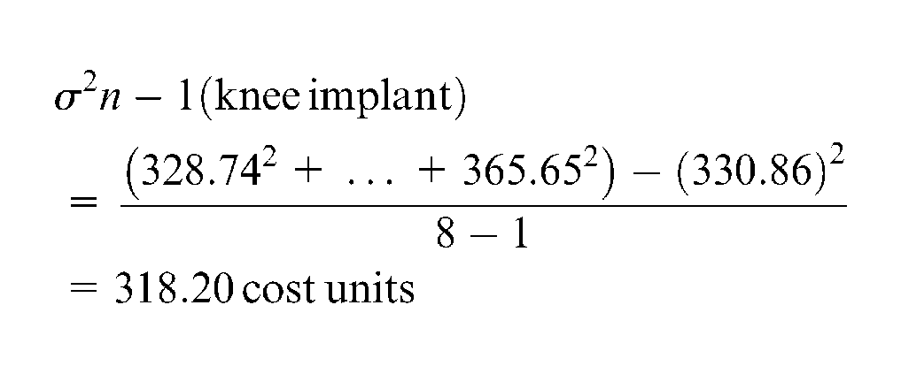
The variance of the manufacturing cost for concept 01 was

$${\sigma }^{2}n-1=\frac{\Sigma y^2-n{Y}^2}{n-1}=\frac{({y_1}^2+\dots +{y_n}^2)-{\left(Y\right)}^2}{n-1}$$

(2)

where

Y is the average manufacturing cost (from equation (1))

y₁ is cost of experiment 1

y_n is cost of experiment n

n is number of experiments

Therefore, from equation (2)

$$\begin{array}{c}{\sigma }^{2}n-1\left(\text{knee}\text{implant}\right)\hfill \\ =\frac{(328.74^2+\dots +365.65^2)-{(330.86)}^2}{8-1}\hfill \\ =318.20\text{cost}\text{units}\hfill \end{array}$$

To summarise the results:

• Average cost before optimisation: 330.86 cost units;

• Variance of cost estimate before optimisation: (σ²): 318.20 cost units;

• σ = 17.83 (SD).

The results indicated that there was a 68% probability that the cost would be within the range of 330.86 ± 17.83 cost units.

Identifying optimum solution

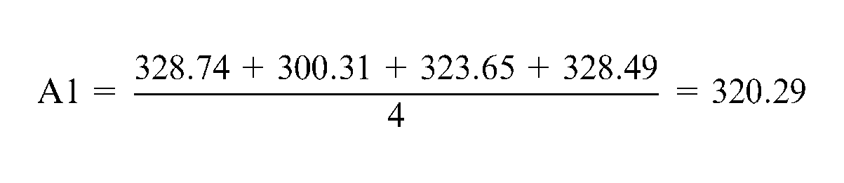
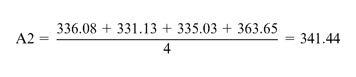
As mentioned, the main aim of this research was to estimate the lowest possible manufacturing cost and the lowest possible variance of the manufacturing cost that designers could achieve by selecting the most appropriate factor levels in the design (while meeting the specifications). To reduce the variance of the manufacturing cost for concept 01, the effect of different levels for each factor was compared. For example, the effect of A1 (level 1 of factor A) and A2 (level 2 of factor A) was compared by taking the average of the effect in those experiments using A1 (experiment numbers 1, 2, 3 and 4) with the average for experiments using A2 (5, 6, 7 and 8). Using Table 7, the average effect of the levels for factor A for concept 01 was

$$\text{A}1=\frac{y_1+y_2+y_3+y_4}{n}$$

(3)

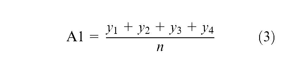
Therefore, from equation (3)

$$\text{A}1=\frac{328.74+300.31+323.65+328.49}{4}=320.29$$

$$\text{A}2=\frac{y_5+y_6+y_7+y_8}{n}$$

(4)

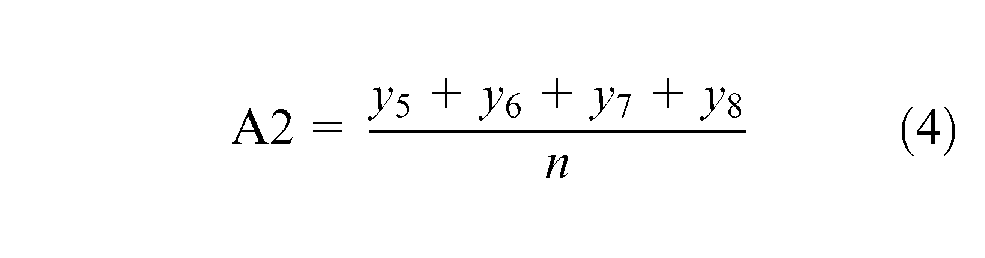
Therefore, from equation (4)

$$\text{A}2=\frac{336.08+331.13+335.03+363.65}{4}=341.44$$

The effect of levels 1 and 2 for other factors (B, A × B, C, D, E and F) was similarly calculated. These results were then added to the response table, shown in Table 8. The difference between level 1 and level 2 of each factor was calculated, and factors with the highest difference ranked as the factors that had the greatest impact on the manufacturing cost for concept 01. As shown in Table 8, factor A (height adjustment) had the greatest impact, and factor F (ability to cut) and factor C (ankle clamp) had the smallest impact on the cost.

Table 8.

The response table for concept 01.

	A	B	A × B	C	D	E	F
Level 1	320.29	324.03	331.93	330.84	336.79	339.21	330.84
Level 2	341.44	337.70	329.80	330.89	324.94	322.53	330.89
Difference	21.15	13.67	2.13	0.05	11.85	16.68	0.05
Rank	1	3	5	6	4	2	7

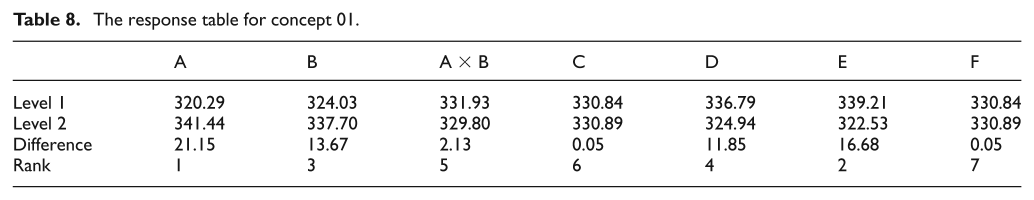
The next stage was to select the most appropriate levels for each factor to reduce the variance of the manufacturing cost. As a rule of thumb, ³⁰ half of the factors (A, E and B) that had the greatest impact on the variance of the cost for concept 01 should be selected.

One level for each of these factors needed to be fixed to reduce the variance. From the results shown in Table 8, the most appropriate factor levels to reduce cost were A1, E2 and B1. However, as lower cost does not necessarily mean better performance an optimisation between performance and cost was carried out. Factor A was rated 5 in terms of performance (shown in Table 2), so although selecting A1 could give the lower cost, A2 was selected to fulfil the performance requirement (this decision was undertaken with the industrial partner, where they believed meeting the desired performance would be a main driver). In the case of factors E and B, since they were rated 4 and 3 (Table 2), respectively, in terms of performance and 2.00° and 390 mm still met the performance requirement, E2 and B1 were selected. Therefore, the optimum solution for concept 01 was A2, E2 and B1.

Calculating the average and variance of manufacturing cost of concept after optimisation

After carrying out the trade-off and selecting the most appropriate levels, the next step was to select the most appropriate orthogonal array to analyse the remainder of the factors (C, D and F) after initial optimisation. Since three factors in two levels (levels 1 and 2) needed to be examined, the standard L4 (2³) orthogonal array was selected and the manufacturing cost of concept 01 for each experiment calculated, as shown in Table 9.

Table 9.

Orthogonal array and unit cost for concept 01 after optimisation.

Experiment	C	D	F	Unit cost
1	90	1.5	7	331.10
2	90	2.0	10	319.35
3	100	1.5	10	331.15
4	100	2.0	7	319.36

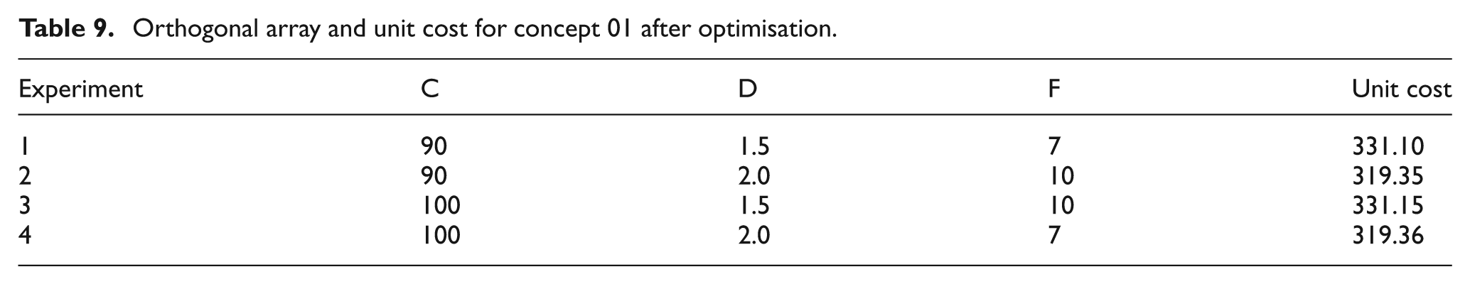
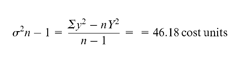
The last stage of phase 2 of the specification/cost trade-off methodology was to calculate the average and variance of the manufacturing cost of concept 01 after optimisation. The average manufacturing cost for concept 01 after optimisation was

$$\begin{array}{cc}\multicolumn{1}{c}{\overline{Y}}& =\frac{331.10+319.35+331.15+319.36}{4}\hfill \\ \hfill =325.24\text{cost}\text{units}\end{array}$$

The variance of the manufacturing cost for concept 01 was

$${\sigma }^{2}n-1=\frac{\Sigma y^2-n{Y}^2}{n-1}==46.18\text{cost}\text{units}$$

To summarise the results after optimisation:

• Average cost after optimisation: 325.24 cost units;

• Variance of cost estimate (σ²): 46.18 cost units;

• σ = 6.79.

This result indicated that with the smaller SD, the average cost would now have a 68% chance of being within the range 325.24 ± 6.79, an improvement of 90%.

Table 10 summaries the average and variance of the manufacturing cost of concept 01 before and after optimisation. It shows that the average manufacturing cost before optimisation was 330.86 cost units, and after optimisation, the average manufacturing cost had reduced to 325.24 cost units. Also the variance of the manufacturing cost for concept 01 was reduced from 318.20 to 46.18 cost units. The optimum solution showed the lowest possible cost and the lowest possible variance of the cost that the designers could achieve by selecting appropriate factor levels for concept 01 (while meeting the specifications).

Table 10.

The average and variance of manufacturing cost for concept 01 before and after optimisation.

Before optimisation		After optimisation
Cost	Variance	Cost	Variance
330.86	318.20	325.24	46.18

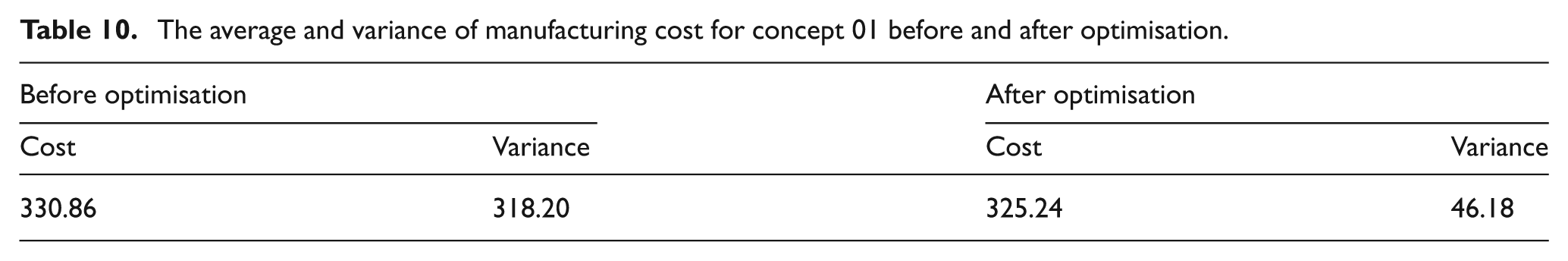
It is important to note that the variance of the manufacturing cost for concept 01 was reduced because the most appropriate values (levels) for factors/metrics A, B and E (factors that had the greatest impact on the product cost, Table 2) were selected and fixed. The variance of the manufacturing cost for concept 01 could be lower if further optimisation was carried for the remaining factors/metrics (C, D and F) and if their values were fixed. But since the effect of the remaining factors/metrics (C, D and F) on the product cost were low, their values need not be fixed at this point (expressed in a range of values). This can assist the designers to have more options in the next stage of design (embodiment or detail) to improve the product design.

To check if the average manufacturing cost would be within the predicted limit (325.24 ± 6.79), further optimisation for the remaining factors (C, D and F) was undertaken. Using Table 9 and the importance ratings in Table 2, optimisation between performance and cost was carried out. In the case of factors C and F, since they were rated 3 (Table 2) in terms of performance and their impact on the product cost was low, C2 and F2 were selected to increase the performance of concept 01. In the case of factor D, although its effect on the product cost was higher than factors C and F, however, because 2.00° still met the performance requirement, D2 was selected. Therefore, the optimum solution for concept 01 was C2, D2 and F2, and the average manufacturing cost for these levels was 319.38 cost units. Since the values of all the factors were now fixed, the variance of the cost estimate was zero.

These results indicated that the final average cost was within the predicted limit (325.24 ± 6.79), estimated in the first round of optimisation. It is important to note that the average cost could be higher if different levels for the remaining factors were selected.

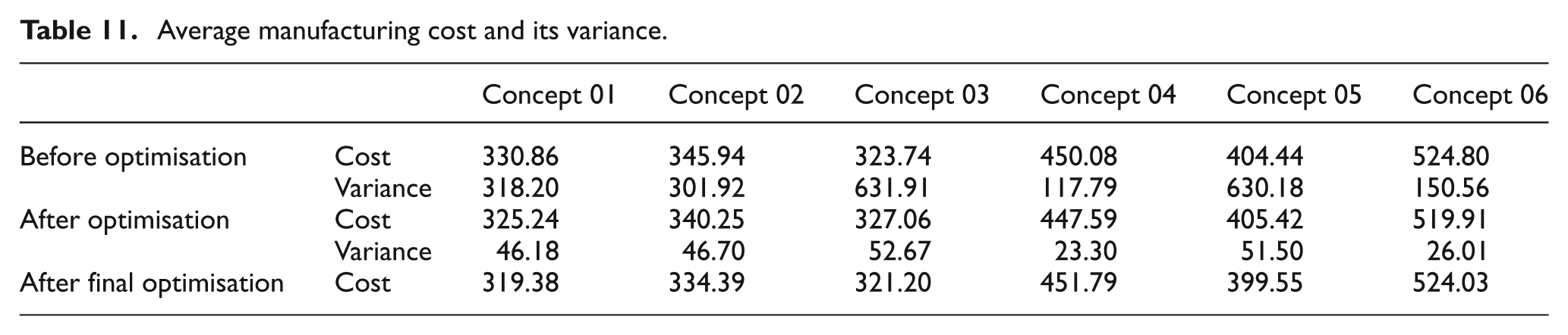
The same method (phase 1 and 2 of the proposed methodology, shown in Figure 5) was used to estimate the lowest possible manufacturing cost with the lowest possible variance for the other concepts (concepts 02–06), as illustrated in Table 11.

Table 11.

Average manufacturing cost and its variance.

		Concept 01	Concept 02	Concept 03	Concept 04	Concept 05	Concept 06
Before optimisation	Cost	330.86	345.94	323.74	450.08	404.44	524.80
	Variance	318.20	301.92	631.91	117.79	630.18	150.56
After optimisation	Cost	325.24	340.25	327.06	447.59	405.42	519.91
	Variance	46.18	46.70	52.67	23.30	51.50	26.01
After final optimisation	Cost	319.38	334.39	321.20	451.79	399.55	524.03

Phase 3 – selecting the final concept

Comparing results of concepts and selecting the final concept

After estimating the lowest possible cost and the lowest possible variance of the cost for all the six concepts, comparing the results and identifying the most appropriate factors were the next and last stage of the specification/cost optimisation process presented in this article. To compare the cost and variance of the cost for each of the concepts, the results are summarised in Table 11. The average cost and variance of the cost of four concepts (01, 02, 04 and 06) were reduced after optimisation. For concepts 03 and 05, the average manufacturing cost after optimisation was increased. This occurred as factor A had a very high impact on concept 03 and 05 in terms of the cost but as factor A was rated 5 (Table 2) in terms of performance, A2 (micro) needed to be selected. That is why the average cost after optimisation had increased, although the variance of the cost of these two concepts was still reduced.

One of the most interesting outcomes was that the results show that the average cost of concept 03 (323.74) was lower than the average cost of concept 01 (330.86) but after optimisation, this was reversed (03 (327.06), 01 (325.24)). This was again because factor A had a higher impact on the cost of concept 03 compared with concept 01. This indicates the importance of applying this method and carrying out optimisation between performance and cost at the conceptual stage of design.

To select the most appropriate design, concepts 01, 02 and 03 were chosen to be assessed (since the average manufacturing cost for concepts 04, 05 and 06 were above target cost). Comparing results for concepts 01, 02 and 03 after optimisation, the average manufacturing cost and its variance for concept 01 were lower than concepts 02 and 03. Therefore, concept 01 was selected as the final design by the designers.

Conclusion

This article has presented the importance of cost estimation at the early product design stages. A structured approach is presented, which offers a step-by-step process to optimise the specification and manufacturing cost for a mechanical product. The outcomes from the optimisation can then be used for designers/decision-makers to select the most appropriate concept. To validate the process, an industrial case study was undertaken. The results illustrated that by using the optimisation process, the outputs can assist designers with their decision-making by analysing how changing the factor levels (values in the product specification) can affect the product manufacturing cost. The results illustrate that the average manufacturing cost and the variance of the cost for each concept can vary when different values for the factors are selected. The process is also useful for ascertaining when a particular design feature can influence the cost. The process is not intended to select the final design but to enable designers to make evidence-based decisions using a repeatable and robust process. It should also be noted that the exemplar in this article was based on a real design challenge. It is the authors’ view that the process can also be used for more complex products; however, it is recognised that an additional pre-analysis will be required to assist users in selecting the initial factors to consider by, for example, the use of Delphi techniques.

Future work

The proposed process presented in this article was based on selecting the factor levels such that they minimise average cost and reduce variation in the product specification to reduce the variation of the average cost (reducing the distribution of cost estimates). Each estimate of the product cost, for each experiment, is a single point estimate, and the uncertainty in it is unknown. Further research is being undertaken to reduce the uncertainty of each single point estimate. To do this, three-point estimates (least, likely and most) for each component and assembly in SEER-DFM would be required and a similar process of identifying lower level factors for each component introduced.