Sage Journals: Discover world-class research

Abstract

A numerical model, developed for LS-Dyna solver, aimed to study the wedge rolling process is presented in this article. In addition, a comparison is made between the experimental and simulated results in order to set up the numerical model’s definition and simulation parameters. The computational performances are evaluated throughout this article to identify the best practice parameters for cold rolling numerical analysis using wedge tools. For an evaluation of the performances of the numerical model, an experimental system was developed to analyse the process parameters of the complex profiles with grooves formed by wedge tools. The methodologies used to record and evaluate the experimental results and the capabilities of the technique are discussed. For a complete analysis, the material behaviour is described by using a five-parameter strain-hardening law. Both the radial force (process force) and the micro-hardness were measured using the Vickers method on a radial section of the rolled piece. The issues addressing the numerical simulation can be extrapolated to other processes (e.g. riveting, flow forming) as this article provides the required information for the development of reliable numerical models.

Keywords

Wedge rolling rolling condition numerical model model parameters LS-Dyna

Introduction

This article is focused on the numerical analysis of a metal forming process. Although wedge rolling process is analysed, the numerical and technical aspects in this article can be extrapolated for other applications (e.g. riveting, flow forming), and it may provide a contribution to the present achievements in this field.

Cold rolling is widely applied to profiled surfaces like threads, grooves and teeth, which are found in various products used in automotive and aeronautical industry or other consumer goods.

The finite element modelling of the cold rolling process started in the 1990s,¹ but the high volume of calculations and the limited capacity of computers to handle the large amount of data within a reasonable time restricted these studies to the understanding of the deformation process.²

Martin³ used numerical models based on MARC finite element code to investigate the residual stress for a threaded profile obtained by cold rolling. This process was also investigated by Domblesky and Feng^4,5 using numerical models and methods (DEFORM). Among the parameters being investigated are the thread profile, friction coefficient, flow stress and workpiece diameter. Pater et al.⁶ investigated the thread rolling process applied to fixing screws using a numerical model developed for MSC.Super Forge. The work of Kamouneh et al.⁷ was focused on the manufacturing process of different types of helical gear using numerical models developed for Abaqus and DEFORM. Lee et al.⁸ present a methodology for the optimisation of the cross-wedge rolling process using a numerical model presented that can be adapted to a number of parameters, such as the friction coefficient, the spreading and forming angle, used to identify the appropriate working parameters in order to avoid defect formation. The published work of Wang et al.⁹ investigates the ring rolling process using numerical models developed for LS-Dyna, and following the simulation results, they were able to improve the manufacturing process by reducing the rolling time by 28%. Guo and Yang¹⁰ studied the radial–axial ring rolling forming process using numerical models developed for Abaqus. The in-feed method of circular grooves recently investigated by Niţu et al.¹¹ found a good agreement with the results obtained from numerical simulation (performed using Abaqus).

Optimisation procedures can be further developed as Aghchai et al.¹² presented in their work for a manufacturing process involving material forming at high strain ratios.

Concluding this survey, it may be stated that numerical analysis is a powerful and reliable tool for manufacturing process investigation. The accumulated knowledge has enabled the forming industry to improve product performance, service life and process competitiveness. Although specialised finite elements codes are available (e.g. DEFORM, MSC.Super Forge), investigations into the development of numerical models for general-purpose solvers are still ongoing.

This article presents a numerical model developed for an explicit finite elements code pointing to the benefits and shortcomings of this numerical method while detailing the features and the simulation parameters used for reliable results.

This study debuts with the investigation of the material used to manufacture the final products. A five-parameter strain-hardening law was used, which is similar to the most frequently used approach for the analysis and simulation of large plastic deformations¹¹ (e.g. Hollomon, Ludwik, Ludwik–Hartley,¹³ Voce, and Johnson and Cook¹⁴).

For the numerical simulation, LS-Dyna was used, an explicit/implicit general-purpose finite element code that has extended capabilities for three-dimensional (3D) modelling of rigid plastic parts, material modelling, finite element definitions and forming capabilities and supports parallel computing. The finite element modelling of cold rolling uses numerical models of the parts involved in the working process (workpiece and tools), with the aim of computing the evolution of different quantities during the process: forces (radial), stresses, strains, micro-hardness and the final dimensions of the product.

The validation results are based on forces (radial or process force) and micro-hardness measurements.¹⁵

Material characterisation

The material used in this investigation was AISI 1015 steel.¹¹ To characterise the stress–strain behaviour of the material, the compression test¹¹ was adopted because it can be used at high strain levels (up to an effective strain $\bar{ε} \approx 0.9$ ) as the stress state generated by the cold rolling process is mostly compressive.

Strain-hardening laws involving only three parameters are not able to provide a good account of the stress–strain curve in the test over the whole range (up to $\bar{ε} \approx 0.9$ ); thus, a five-parameter law was selected. This law combines Hollomon and Voce’s laws and expresses the hardening law in the form

σ_{LS} = [K \cdot ε^{n} + S \cdot (1 - A \cdot \exp (- B \cdot ε))]

(1)

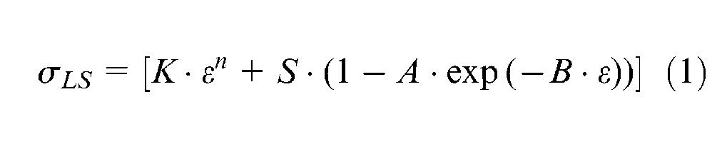
where K, n, S, A and B are material-related parameters.

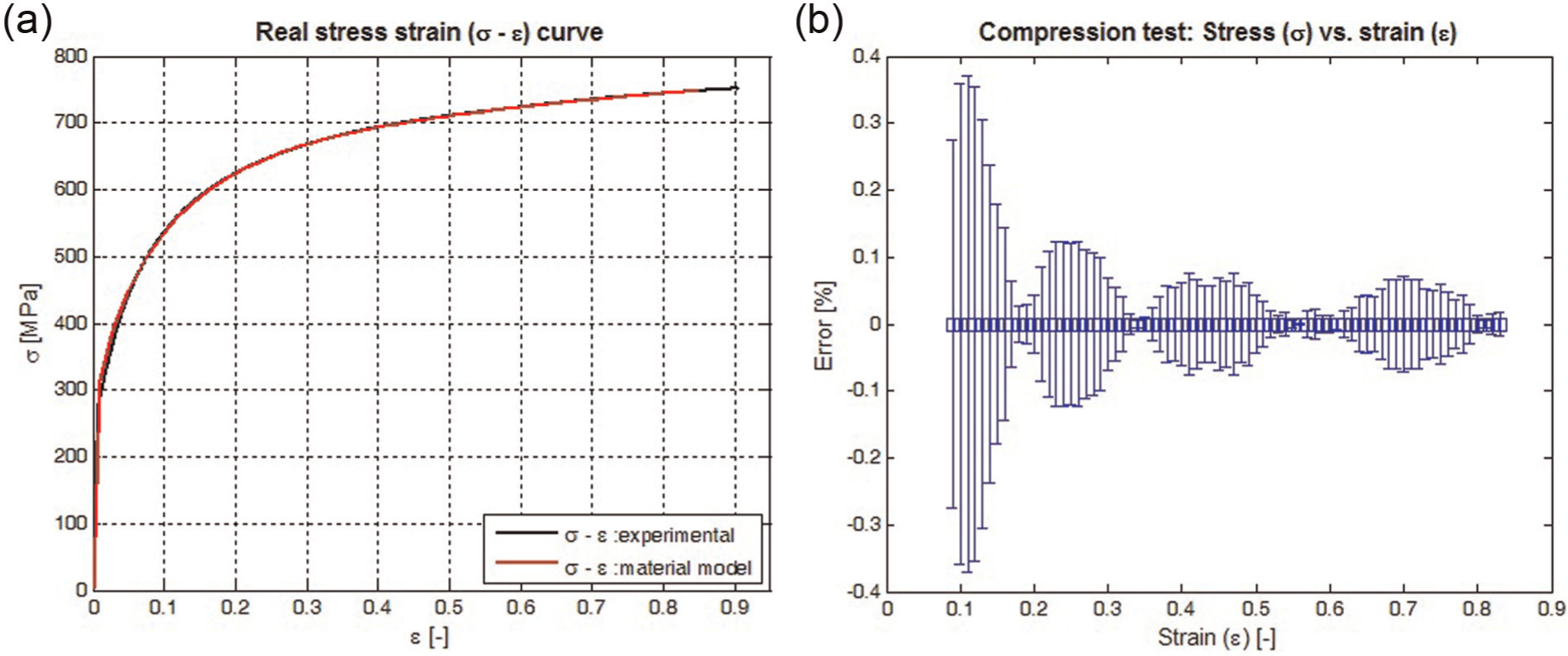
The identification of the five strain-hardening parameters for equation (1) is first performed by fitting the test data¹¹ and the following results were obtained: $K = 542.5 MPa$ , $n = 0.135$ , $K = 217.6 MPa$ , $A = 0.99$ and $B = 9.91$ . The resulting stress–strain curve is presented in Figure 1(a). Figure 1(b) presents the computed error between the measured (real) stress–strain curve and the analytical (equation (1)) stress–strain curve. Note that the maximum recorded error is 0.4%, with a global tolerance of 0.1%.

Figure 1.

Stress–strain curve: (a) real versus analytical stress–strain curve and (b) the computed error.

Once these parameters were identified, the stress–strain behaviour of the material was completely characterised, and a number of numerical simulations were performed. This step was performed to evaluate and compare the results obtained by numerical simulation with the results obtained from the experimental testing.

The numerical simulation of material testing process was performed using LS-Dyna software. Although the numerical method and models will be discussed in detail in a further section, a brief introduction of the numerical model is necessary. The contact between the moving plate and the specimen was implemented using a standard definition of the surface-to-surface contact interface. The material model for the specimen was set to piecewise linear plasticity, and the stress–strain curve defined by equation (1) was used.

For the moving plate, defined as a rigid structure, a prescribed displacement of 18 mm was set. The simulation time was defined according to the required plate travel of 18 mm and the prescribed test velocity.

The specimen was modelled using 3D solid elements. The mathematical model of the finite element modelling can be set by the ELFORM parameter that is defined on the *SECTION_SOLID card.

Two formulations were used: an under-integrated constant stress element (ELFORM = 1), further referenced as Model I, and a fully integrated solid element (ELFORM = 2), further referenced as Model II. For the under-integrated finite element (Model I), hourglass control had to be enabled.¹⁶

Figure 2(a) presents the shape of the specimen after the compression test. Figure 2(b) presents the shape of the specimen determined by the numerical simulation.

Figure 2.

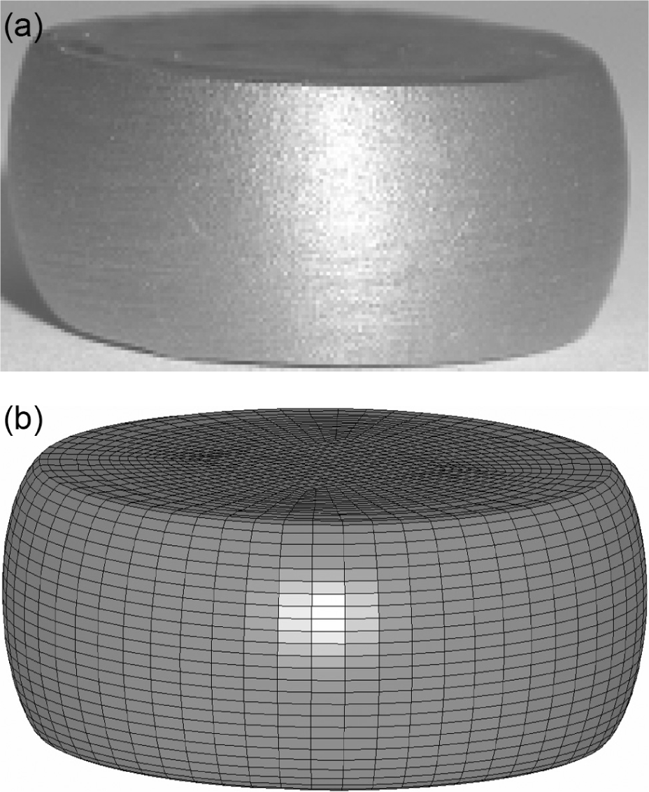
Shape of the specimen: (a) after the compression test and (b) the numerical simulation result.

The compression test was simulated, and the deformation force, measured at the contact interface, was recorded. The results obtained for the compression test are presented in Figure 3. Figure 3(a) presents the measured test forces and the computed test forces and Figure 3(b) presents the computed error.

Figure 3.

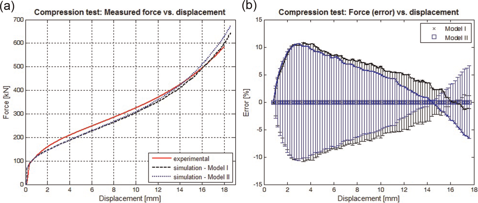
Results of the compression test: (a) deformation force (experimental vs numerical simulation (Model I, Model II)) and (b) computed error.

The maximum calculated error is approximately 10%, and a difference of up to 3% between the different mathematical models of the solid element is recorded. In Figure 3(b), for strain levels above 50%, the under-integrated solid element (Model I) with corrected viscosity (by hourglass control) can predict with satisfactory accuracy the value of the deformation force pointing to this model as a good candidate for the analysis of the forming process.

Experimental work

Process description

The cold rolled parts were obtained using an industrial rolling flat wedge machine. The process is presented in Figure 4(a), and Figure (b) displays the machine used for the experiments.

Figure 4.

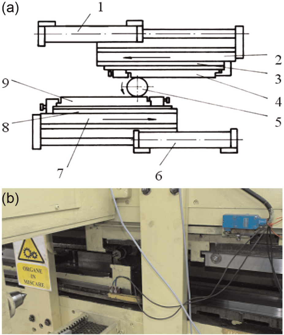
The generation method of the part: (a) schematic view and (b) photograph of the experimental apparatus.

The workpiece (5) is positioned and secured on the machine. The contact is set between the workpiece and the lower and upper flat wedges (4) and (9). The displacements of the two sleds are correlated by a pinion, which engages, with a small clearance, with the wedge tools mounted on the sled. The tools have a prescribed velocity, $v$ , and due to the friction forces developed, the workpiece rotates while the tools are moving. Thus, the profile is obtained by the translational displacement, due to the special construction of the tools. Finally, the two tools are mounted on sleds (2) and (7), actuated by two linear hydraulic motors (1) and (6), and are constrained by the guides (3) and (8).

Experimental research

The processed profiles are circular ones, with the geometry—in an axial section—corresponding to metric threads of general use. The forming depth is the maximum distance of penetration of the wedge tool in the semi-finished products and can be calculated with

h = \frac{d_{0} - d_{i}}{2}

(2)

where $d_{0}$ is the workpiece diameter and $d_{i}$ is the groove diameter of the part (Figure 5).

Figure 5.

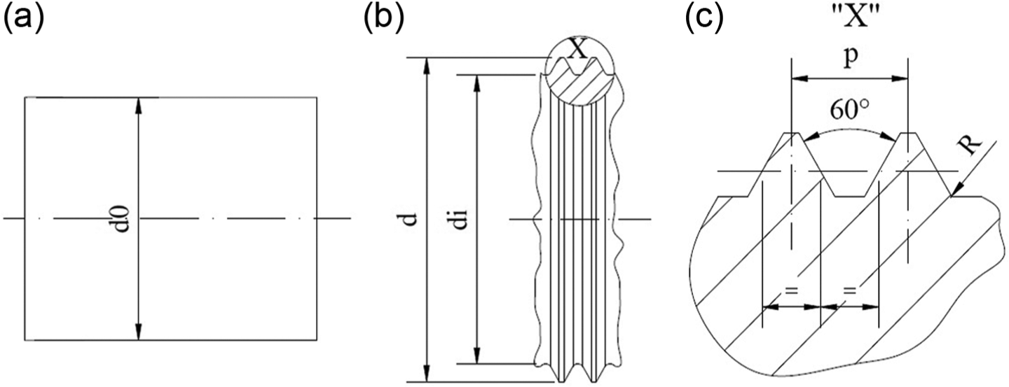
Dimensions of the part: (a) the workpiece, (b) finished part and (c) detailed view of the profile (M20).

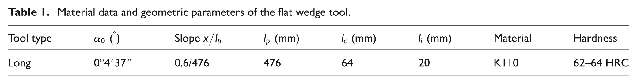
Regarding the tool configuration, the following sections are identified: an inclined section to provide at least one rotation for the part (l_p, Figure 6), a section without tilting to achieve the profile circularity (l_c, Figure 6) that must provide at least 0.5 turns of the part and a reverse slope part (l_i, Figure 6) to ensure the spacing of the part from the wedge tool by the cancelling of the elastic forming in the system. The slope of the wedge tool is provided by the construction of the tool. The tool has a total length of 560 mm. The slope angle has a value of $0^{\circ} 4' 37 ″$ . The constructive elements of the tools are presented in Figure 6 and Table 1.

Table 1.

Material data and geometric parameters of the flat wedge tool.

Tool type	$α_{0} (^{\circ})$	Slope $x / x l_{p}$	$l_{p} (mm)$	$l_{c} (mm)$	$l_{i} (mm)$	Material	Hardness
Long	0°4′37″	0.6/476	476	64	20	K110	62–64 HRC

Figure 6.

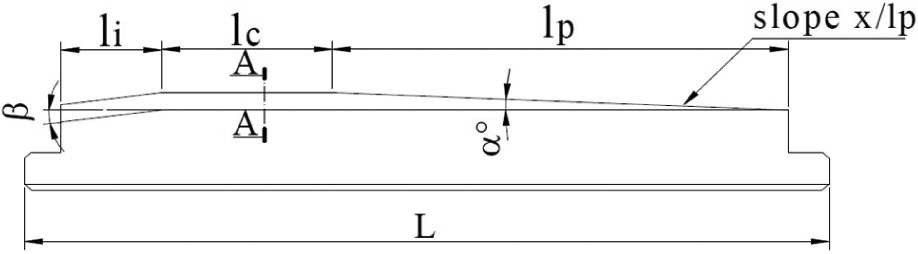
Flat wedge tool construction.

The rolling force, the process parameter examined, is a plane force with two components: radial component, F_r, and tangential component, F_t , (Figure 7) as determined by the formula

F = \sqrt{F_{t}^{2} + F_{r}^{2}}

(3)

Figure 7.

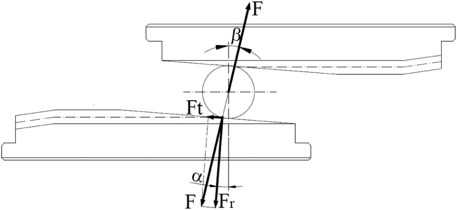
Rolling force components.

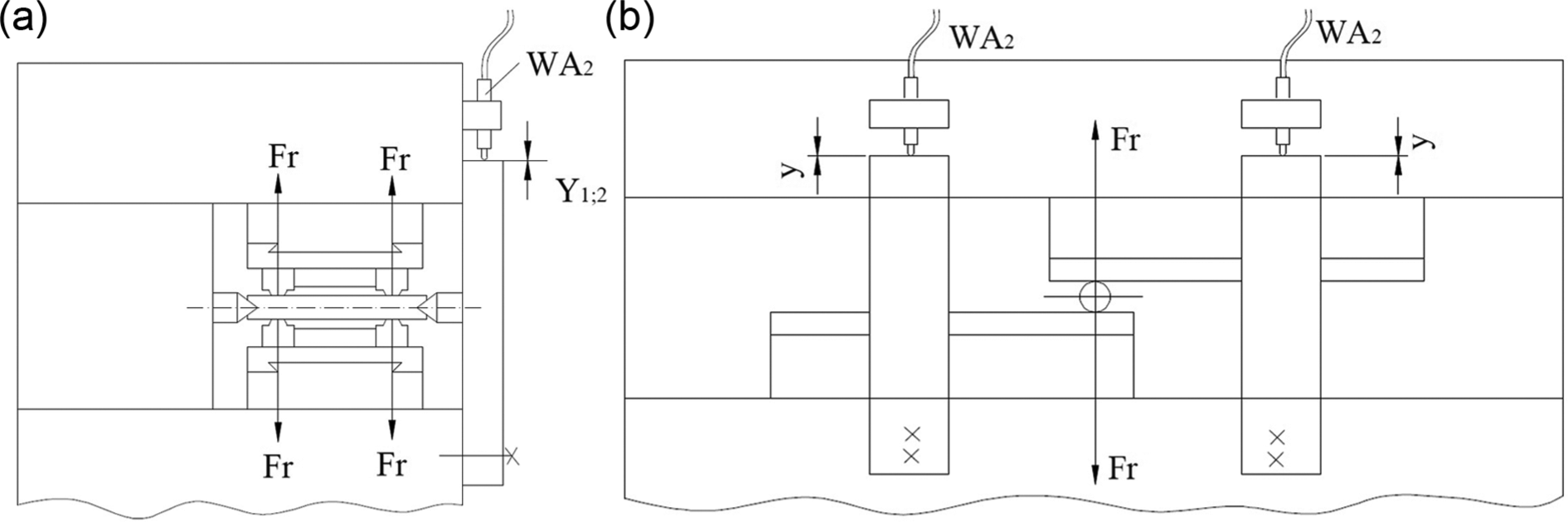
The main component is the radial force, $F_{r}$ , that produces the radial displacement of the material. The tangential component, $F_{t}$ , is significantly smaller due to the values of the angles, $α$ and $β$ , which produce a rotational motion of the workpiece about its axis and cause a material shift in the tangential direction. The measurement of the radial forming force component, $F_{r}$ , was performed by measuring the displacement of support of the flat rolling wedge (Figure 8).

Figure 8.

Measurement of the radial force: (a) side view and (b) front view.

The measurement process takes into consideration the fact that in a run, on the same flat wedge are processed successive profiles with both wedge tools and that the wedge tools are displaced by 110 mm in between. Vertical tool displacements are measured with two inductive displacement transducers, WA₂, mounted symmetrically against the part to be rolled.

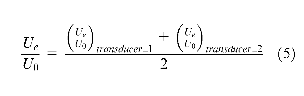
A known radial force was applied using a mechanical system (screw and nut), and the value of the force was measured using a load cell (maximum load 200 kN, sensitivity 2 mV/V, deviation from linearity below 0.1%). The signals from the displacement transducers were recorded. To calculate the force in the equation of calibration, the averaged value of the electrical signals recorded from the two transducers was used. Therefore, the equation of calibration can be written as follows

F = 15.6285 \cdot (U_{e} / U_{0})

(4)

where $U_{e}$ is the output (recorded) value, $U_{0}$ is the input (supply) value and ratio $U_{e} / U_{e} U_{0}$ is the averaged value of the signal recorded from the displacement transducers

\frac{U_{e}}{U_{0}} = \frac{{(\frac{U_{e}}{U_{0}})}_{transducer_1} + {(\frac{U_{e}}{U_{0}})}_{transducer_2}}{2}

(5)

Experimental results

The data recorded during the experiments were processed, and the resulting radial force history is presented in Figure 9.

Figure 9.

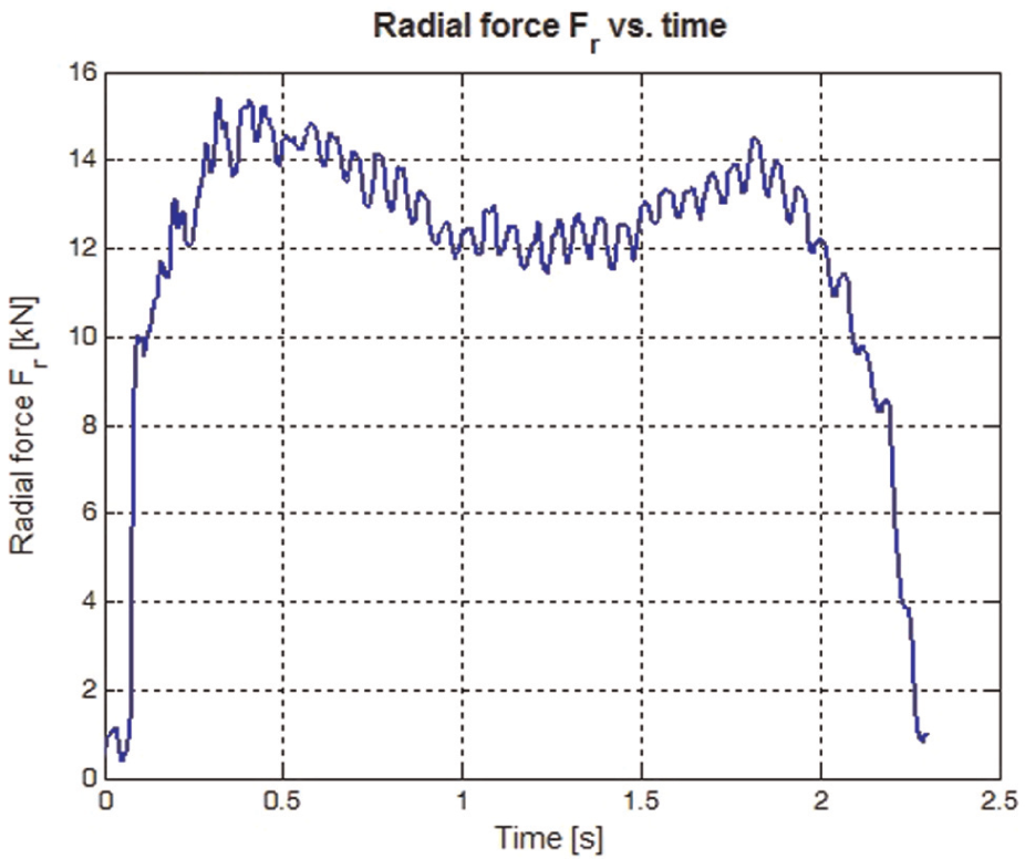
Measured radial (process) force $F_{r}$ versus time.

Micro-hardness measurements were made by the Vickers method, which allows the use of small loads, to compare the results with other mechanical quantities (Figure 10). The load was taken to be equal to 300 g to take into account the estimated micro-hardness and the grain size. The piece was cut, and the micro-hardness in the radial section of the tooth was measured.

Figure 10.

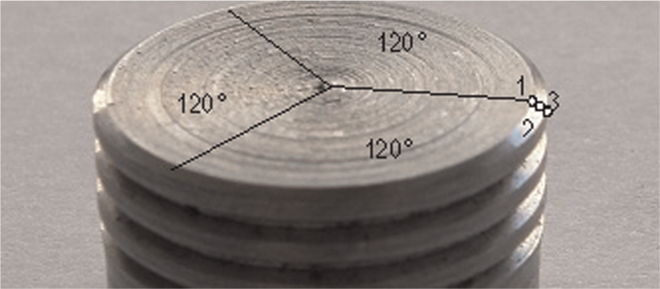
Schema of the micro-hardness indentations.

The measurements were performed at three points located at the bottom, middle and top of the tooth for three radial locations (0°, +120°, +240°). The results are listed in Table 2.

Table 2.

Micro-hardness results.

Measured	0°	+120°	+240°	HV	HV average
1 (bottom)	287	275	275	279	272
2 (middle)	287	263	263	271
3 (top)	263	275	263	267

Numerical model and simulation prerequisites

The numerical simulations were performed using the general-purpose finite element explicit solver LS-Dyna in the ANSYS ACADEMIC RESEARCH LS-Dyna package. The machine used for running the simulations has an Intel-based architecture with a Dual Xeon QUAD Core (E 5620) CPU running at 2.4 GHz. The machine has a total installed RAM of 12 GB. The operating system is Windows 7, 64 bits architecture. The existing infrastructure provided the necessary support to run the simulations using massively parallel processing (MPP) features available in LS-Dyna. A number of issues related to the numerical simulation will be further discussed and analysed with respect to the performance of the numerical simulation.

Units

The system of units that was defined for the numerical simulations is presented in Table 3.

Table 3.

Units.

Mass	Length	Time	Force	Stress	Energy	Density (kg/mm³)	Young’s (GPa)	Gravity (mm/ms²)
kg	mm	ms	kN	GPa	kN mm	7.85e−6	2.10e2	9.81e−3

Numerical model

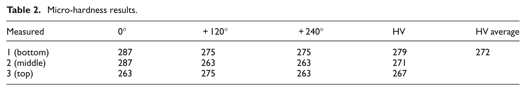
The numerical model used in this study is presented in Figure 11. The size of the finite element is closely related to the configuration of the tool. Figure 11(a) is an overview of the numerical model displayed at the beginning of the simulation time. Figure 11(b) presents a detailed view of the numerical model at the interface between the workpiece and the tool. The number and size of the finite element were defined with respect to the interface between the workpiece and the tool to ensure that there will not be any highly distorted elements during the simulation and that for each segment of the tool defined in a transversal cut, there should be a satisfactory number of elements. The width of the finite element (measured along the axis of the workpiece) is 0.125 mm. The model has a total number of 33,400 shell elements, for the tool and the contact interface (quadrilateral), and 196,800 solid elements, for the workpiece model (190,464 hexahedral elements and 6336 pentahedral elements).

Figure 11.

Numerical model: (a) overview of the numerical model and (b) detailed view of the interface (tool–workpiece).

Time step and simulation time

There are two methods to solve the numerical problems. The explicit formulation has the benefit of solving a system equation for each unknown displacement, while the implicit formulation solves a set of equations using matrix operations. The explicit formation requires the time step to be smaller than a critical value defined by a model metric and material properties. The implicit formulation does not require a critical time step but there is a high computational cost due to the matrix assembly and solve. For numerical problems with an increased number of elements (high number of degrees of freedom), this may not be a feasible method unless high performance computing machines (large amount of RAM) are available. Using the computing machine presented above, the computational requirements of the implicit method were not matched by available resources; therefore, the only available solution was the explicit method.

With respect to the system of units that was selected for the numerical analysis with the chosen finite element size, the time step can be defined as

Δ t = \frac{l_{min}}{c_{steel}}

(6)

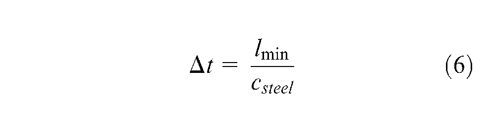
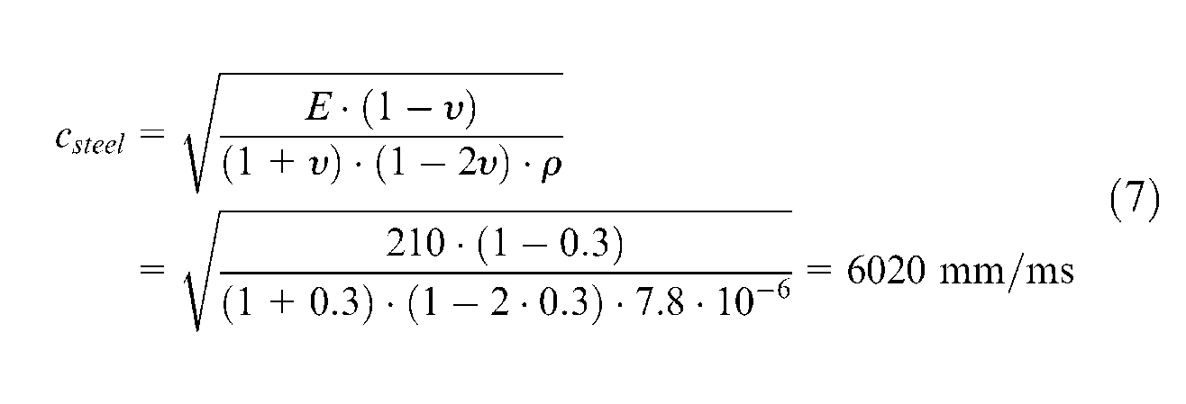
where $l_{min} = 0.125 mm$ is the minimum edge length of the finite elements (current model) and $c_{steel}$ is the sound velocity in the material.

The sound velocity is

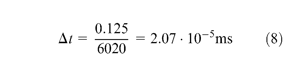
\begin{matrix} c_{steel} & = \sqrt{\frac{E \cdot (1 - υ)}{(1 + υ) \cdot (1 - 2 υ) \cdot ρ}} = \sqrt{\frac{210 \cdot (1 - 0.3)}{(1 + 0.3) \cdot (1 - 2 \cdot 0.3) \cdot 7.8 \cdot 10^{- 6}}} = 6020 mm / ms \end{matrix}

(7)

The time step size is

Δ t = \frac{0.125}{6020} = 2.07 \cdot 10^{- 5} ms

(8)

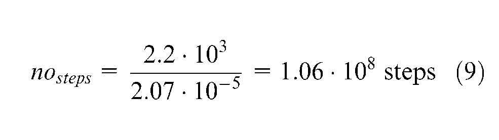
From the experimental results, the calculated fabrication time is 2.2 s (Figure 8), so the total number of steps is

n o_{steps} = \frac{2.2 \cdot 10^{3}}{2.07 \cdot 10^{- 5}} = 1.06 \cdot 10^{8} steps

(9)

The average CPU time (on our machine) for each time step is 0.5 s. Therefore, the runtime will be

runtime = 1.06 \cdot 10^{8} \cdot 0.5 s

(10)

or approximately $14 \cdot 10^{3} h$ , which is an unacceptable runtime.

The simulation time needs to be adjusted in order to fit the requirements of the computational model and to fit the available hardware resources. The first step is to reduce the simulation time from seconds to milliseconds. The runtime is

runtime = 1.06 \cdot 10^{5} \cdot 0.5 s

(11)

resulting in a total runtime of approximately 14 h.

By translating the simulation time from seconds to milliseconds in order to match the computational resources, the total energy will also be scaled. Starting from 2.2 ms, by scaling this value using integer values (e.g. 3, 5), the resulting simulation times of 6.6 and 11 ms were obtained, and a number of runs were performed to select the most satisfactory simulation time.

The deformation force was computed and the resulting time histories are presented in Figure 12. The time values were normalised with respect to the final simulation time.

Figure 12.

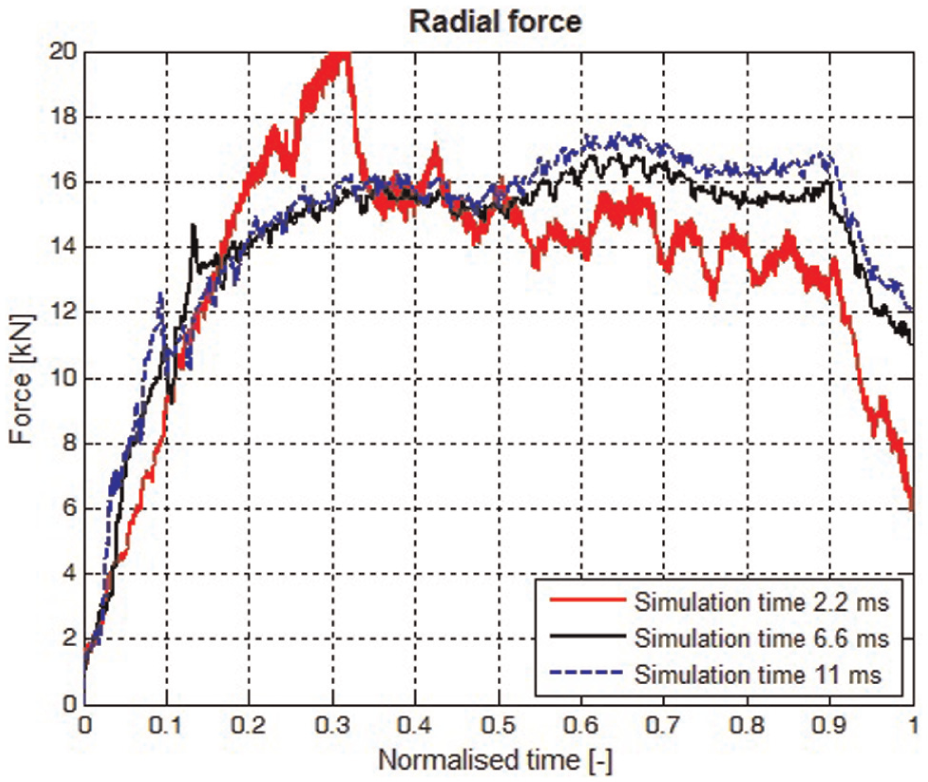
Deformation force. Simulation time 2.2, 6.6 and 11 ms (normalised time).

The history of the calculated force for 6.6 and 11 ms is similar in terms of the value and the shape, but the history of the calculated force for a simulation time of 2.2 ms displays large variations in terms of the shape and the values from the previously presented force histories (Figure 13). Following this remark, the total simulation times were set to 6.6 and 11 ms, and complementary results were further analysed.

Figure 13.

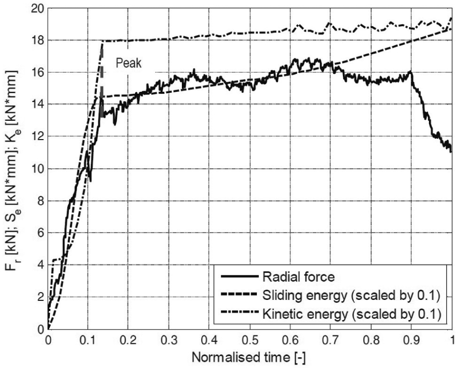
Radial force, sliding and kinetic energies for the 6.6-ms simulation.

Contact interface

To benefit from the forming capabilities implemented in LS-Dyna, the contact interface was set to a surface-to-surface model (FORMING_SURFACE_TO_SURFACE), and the value of the coefficient of friction was set to 0.3. In this case, a surface was generated on the workpiece cylindrical surface. The material model of this surface was set to *MAT_NULL, so it will have no influence over the workpiece model; however, to ensure the required contact conditions, Young’s modulus and Poisson’s ratio for this material are used only to set the contact interface stiffness.

Solid element

As previously mentioned, two mathematical formulations for the finite elements of the workpiece were selected and analysed for this article. The first mathematical model (under-integrated constant stress solid/one point integration) is set by a value of the ELFORM parameter of 1 (currently defined as Model I). This mode is efficient (in terms of computational resources), accurate and behaves well even in the case of severe deformations. One shortcoming of the under-integrated model is that it requires hourglass stabilisation (by using the *CONTROL_HOURGALSS card), thus adding a non-physical measure that has to be evaluated. Hourglass stabilisation is performed by the addition of internal forces to the element¹⁷ in order to control the deformation of the under-integrated elements. The viscosity type (IQH parameter) and the hourglass coefficient (QH parameter) depend on the problem to be solved. For the current application, the viscosity type was set to 5 (stiffness of type 3), and the hourglass coefficient was varied from 0.15 to 0.05. Finally, a value of 0.10 (recommended for most application) was used.

The second mathematical model, the fully integrated solid element, is set by assigning a value of 2 to the ELFORM parameter (currently defined as Model II). This element model does not need hourglass stabilisation, but due to the additional computational effort, the runtime increases. Another shortcoming of this model is that there are cases when it becomes too stiff, due to shear locking,¹⁷ for models with poor aspect ratios of the elements¹⁶ or for large deformations.

The model with fully integrated elements (Model II) is used as a benchmark for the stress and strain analysis and to evaluate the effect of hourglass stabilisation required by the under-integrated elements.

Material model

The material was considered as isotropic. The parameters describing the elastic behaviour are those generally defined with the following values: Young’s modulus, E = 210,000 MPa, and the Poisson’s ratio, $υ = 0.3$ . For the strain hardening, von Mises criterion with isotropic hardening was used and the yield function is given by

f = \sqrt{\frac{3}{2} s_{ij} s_{ij}} - \bar{σ}

(12)

where $s_{ij}$ are the deviatoric stress components, $\sqrt{(3 / 2) s_{i j} s_{i j}}$ is the von Mises equivalent stress and $\bar{σ}$ is the current yield stress. The law obtained in the compression test (section ‘Material characterisation’) was used to describe the stress–strain behaviour of the material for the numerical simulations.¹¹

For the workpiece, the material was set to the piecewise linear plasticity model (*MAT_24), while the tools were modelled using rigid material. Rigid material provides the capabilities of constraining a user-defined number of translational and rotational degrees of freedom of the part.

Results and discussion

One of the major benefits of the numerical simulation method is that it provides results for a large number of time histories of different parameters that are in some cases very difficult to measure using experimental equipment.

The numerical models were set to evaluate during the simulation, among standard parameters (e.g. dimensions, stress and strain), the kinetic energy, internal energy, hourglass energy, sliding (contact) energy and the forces. The time history of the kinetic energy is used to outline the transition from the initial state (stationary) of the workpiece to the nominal working state (constant rotational speed).

Figure 13 presents the sliding and kinetic energies and the radial force obtained from the 6.6-ms simulation. The energies were scaled to fit the scale associated with the radial force.

Figure 14 presents the sliding and kinetic energies and the radial force obtained from the 11-ms simulation. The energies were also scaled to fit the scale associated with the radial force.

Figure 14.

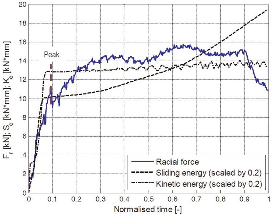
Radial force, sliding and kinetic energies for the 11-ms simulation.

The peaks of the radial force marked in Figures 13 and 14 indicate the end of the transition from the initial state (stationary) to the process rotational velocity of the workpiece by evaluating the slope of the kinetic energy, which is close to horizontal. Combining these results, Figure 15(a) presents the experimentally measured radial force and the computed radial force.

Figure 15.

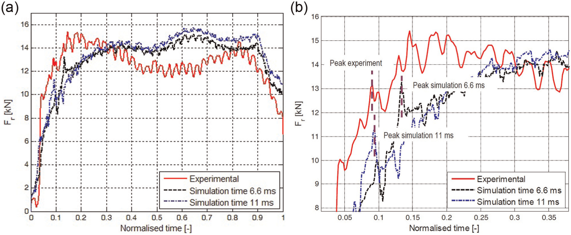
Radial force, experiment versus simulation. Simulation time 6.6 and 11 ms. (a) Histories of the radial force and (b) detailed view.

Note that there is good agreement between the peak location (with respect to the normalised time) for the experimental force and the 11-ms simulation (Figure 15(b)).

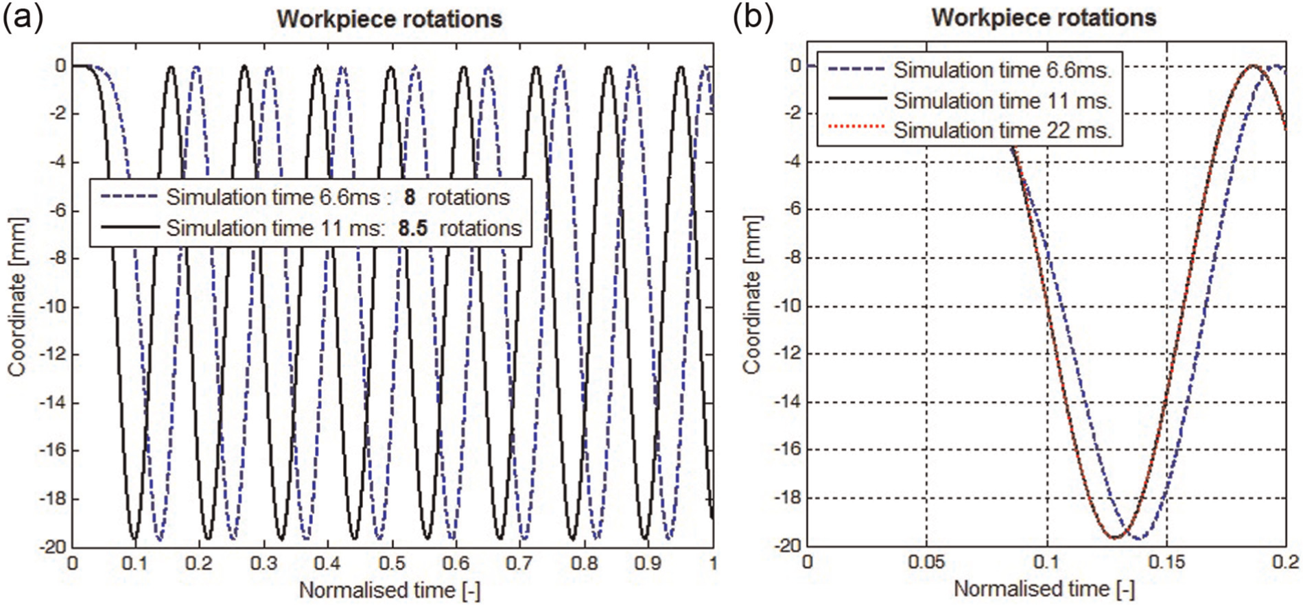
A second parameter that is investigated at this point is the total number of workpiece rotations during the process. The total length of the tool is of 540 mm and the workpiece diameter is 19.717 mm. The change of diameter can be neglected in order to evaluate the number of rotations of the workpiece during the rolling process

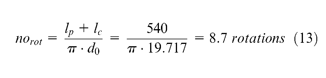
n o_{rot} = \frac{l_{p} + l_{c}}{π \cdot d_{0}} = \frac{540}{π \cdot 19.717} = 8.7 rotations

(13)

Selecting a point on the circumference, the number of workpiece rotations can be calculated using the numerical model. For the model with the simulation time set to 6.6 ms, the number of rotations is 8, while for the model with the simulation time set to 11, the number of rotations is 8.5, which is close to the number predicted by equation (13).

The normalised time when the first half-rotation of the workpiece is completed is in agreement with the location of the marked peak force. Once the first half-rotation is completed, the rotation time (normalised time, Figure 16(a)) for both numerical models is similar. This result (the time when the first half-rotation is completed) is also related to the predicted (and used) value of the coefficient of friction for the numerical model.

Figure 16.

Workpiece rotations: (a) number of workpiece rotations and (b) workpiece rotation after 20% of the simulation time.

The simulation time can be identified by comparing the peak (force) that marks the end of accentuated sliding of the workpiece at the beginning of forming process. Also the rotation of the workpiece is related to this transition. Comparing the results for different simulations with different simulation times, the most reliable value can be identified. In order to validate the simulation time of 11 ms, another simulation with a total process time of 22 ms was set and the run was stopped after 20% of this time. The first workpiece rotation for the mentioned simulation times are presented in Figure 16(b)) showing a close match with the values recorded for the 11-ms simulation. Therefore, for the preliminary phases of model development and results evaluation, it is not required to complete the entire selected simulation time as it can be performed only up to about 20% of this value. This is a considerable advantage when the time required for the development of the numerical model is addressed.

Following these preliminary results, the simulation time of the process was set to 11 ms, and the model was solved using the MPP capabilities of LS-Dyna and using a total number of 8 CPUs assigned to the job.

The experimental and simulated histories of the radial force are presented in Figure 17 in order to evaluate the performance of the numerical models. This figure is useful because the radial force is a parameter of interest when the wedge rolling process is analysed, thereby providing information that can be used for the evaluation of the tool lifetime.

Figure 17.

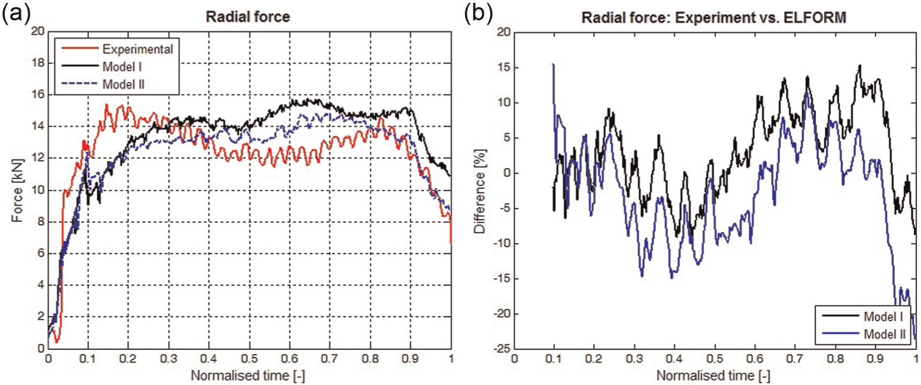
Radial force: (a) Model I versus Model II and (b) the calculated difference.

In Figure 18, the final shape of the model is presented; note that there are no distorted elements (due to contact interface). In Figure 19, the shape of the part is presented as obtained from the manufacturing process.

Figure 18.

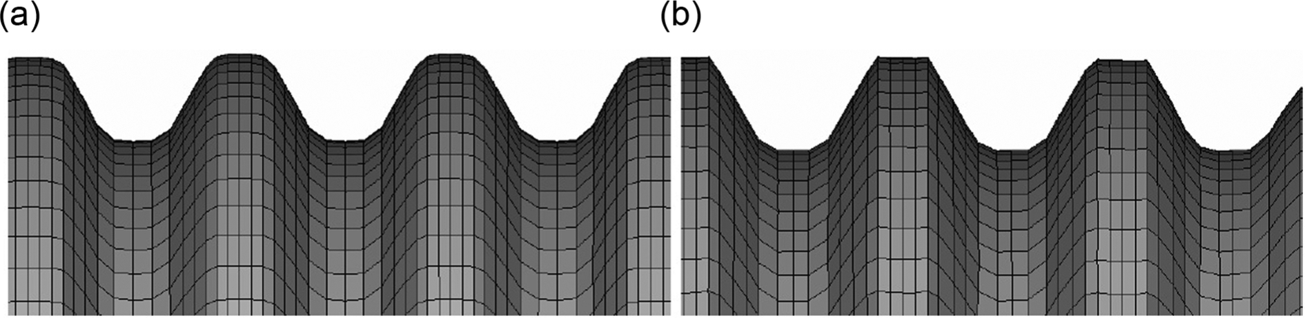
Deformed shape: (a) Model I and (b) Model II.

Figure 19.

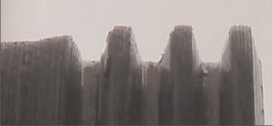
Part (obtained from the manufacturing process).

The bottom shape of the teeth is more rounded for the numerical models than in the experimental part due to the contact definition and the number of solid elements defined, yet a rounded shape of the top of the tooth is obtained for both the numerical models and the experimental part. The top of the tooth is sharper for the model that uses the fully integrated solid element (Model II).

In Figure 20, the stress state of the part is presented. The stress state displayed by the model using the constant stress model is closer to the real case. The average stress recorded is of 450 MPa (0.45 GPa)

Figure 20.

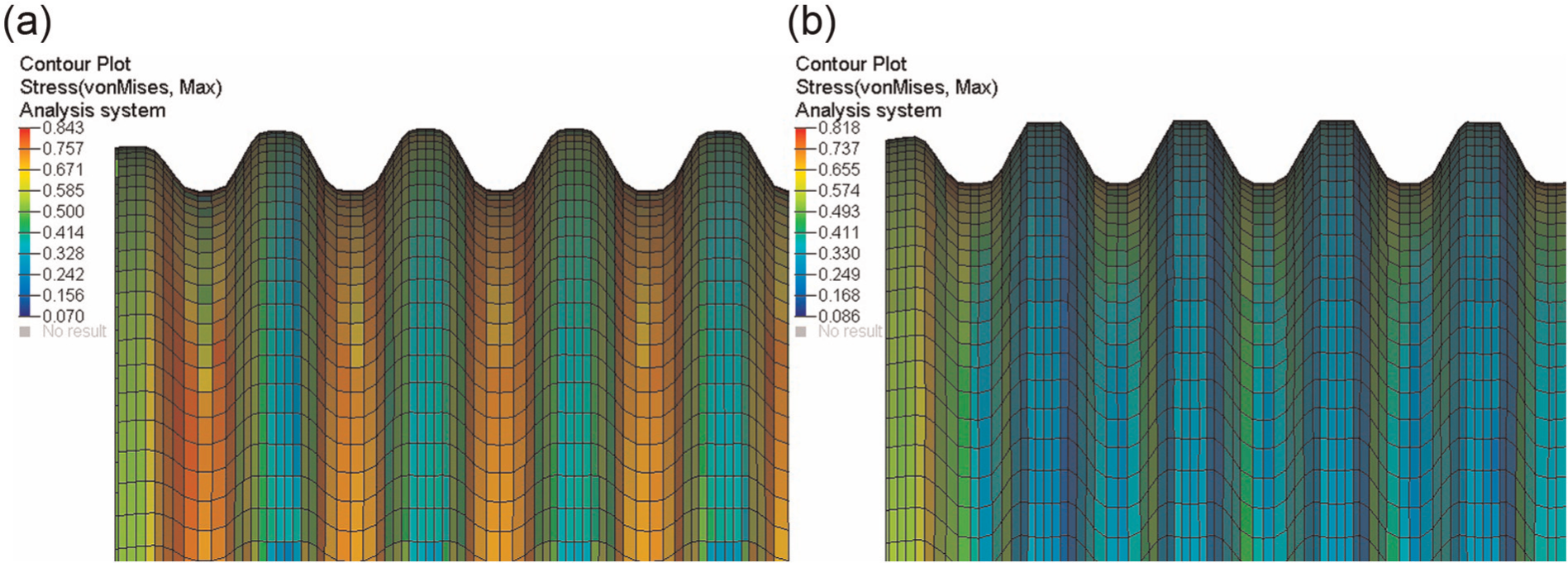
Stress state (von Mises, GPa): (a) Model I and (b) Model II.

In Figure 21, the strain state (plastic strain) of the part is presented. The dimensions of the final models, as obtained from the numerical simulations, are presented in Figure 22.

Figure 21.

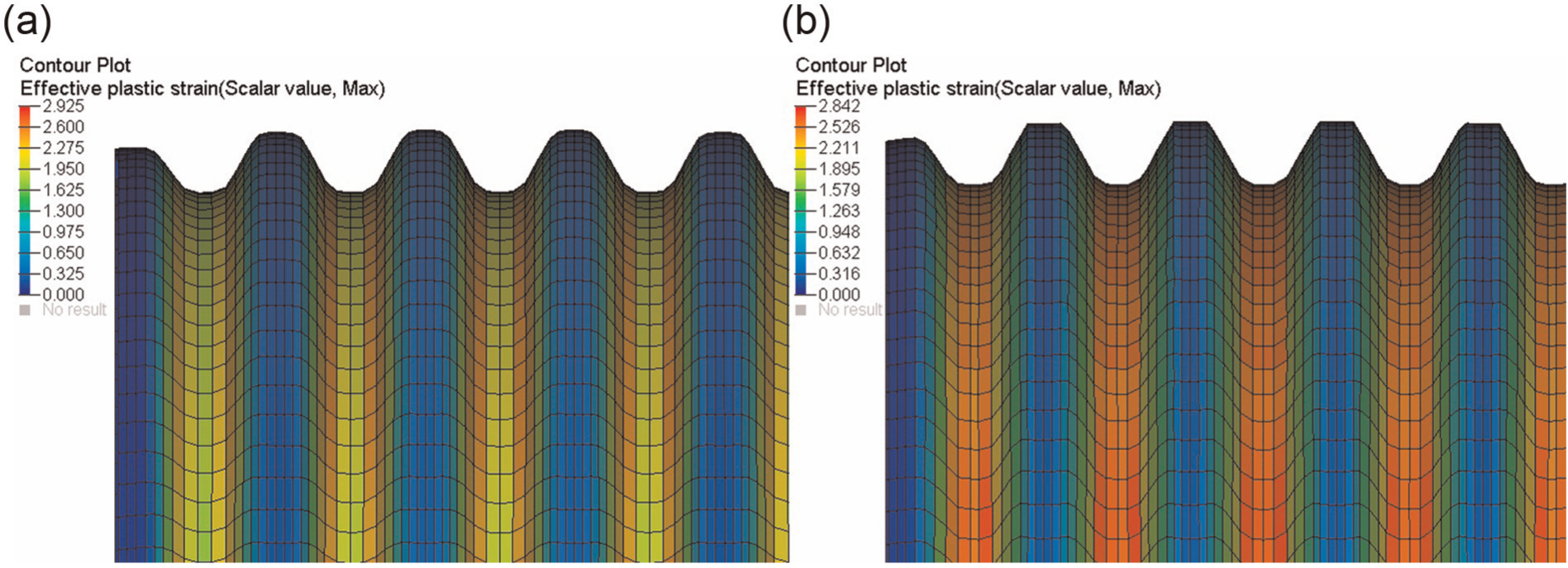
Strain state (plastic strain (–)): (a) Model I and (b) Model II.

Figure 22.

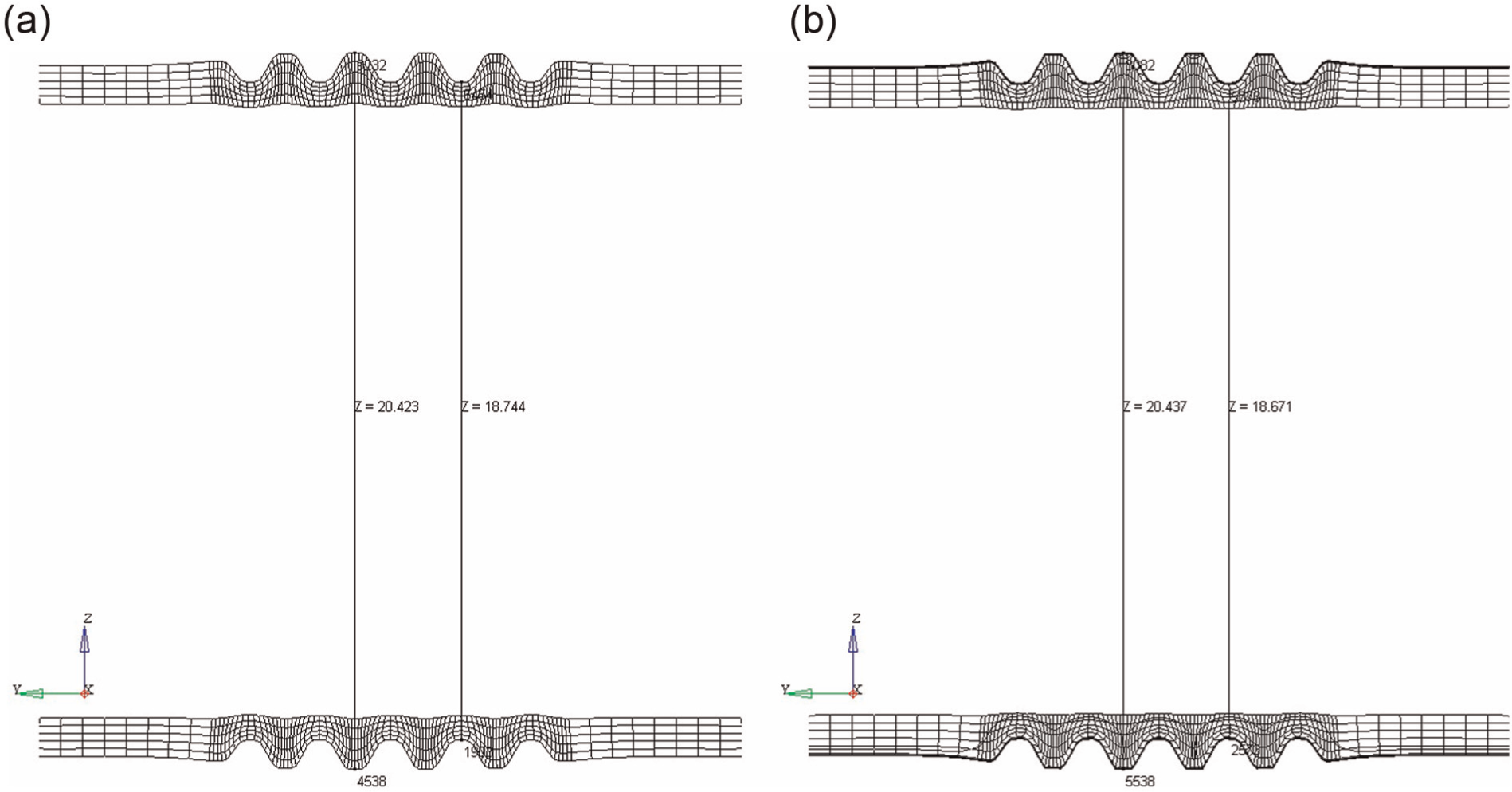
Dimensions of part (end of process): (a) Model I and (b) Model II.

The dimensional results are summarised in Table 4. For blank materials, the Vickers micro-hardness HV is found to be proportional to the initial yield stress σ_y¹²

Table 4.

Dimensional results (mm).

	Part	Model I	Model II
Workpiece diameter	19.717	19.7	19.7
Outer diameter (d)	20.136	20.429	20.437
Inner diameter (d_i)	18.807	18.744	18.671

H V = α \cdot σ_{y}

(14)

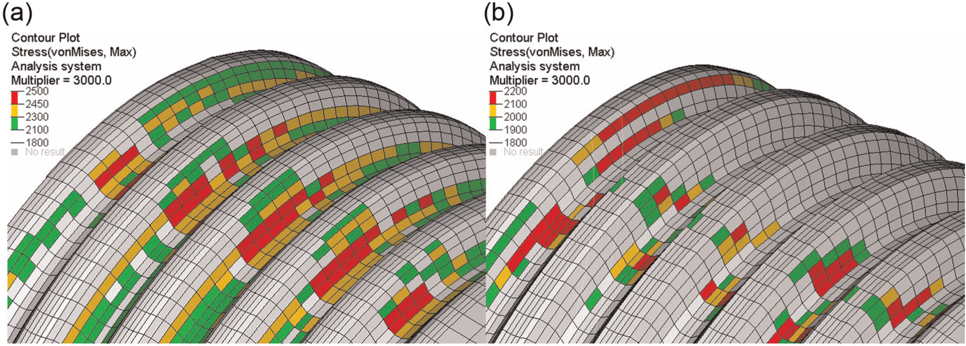
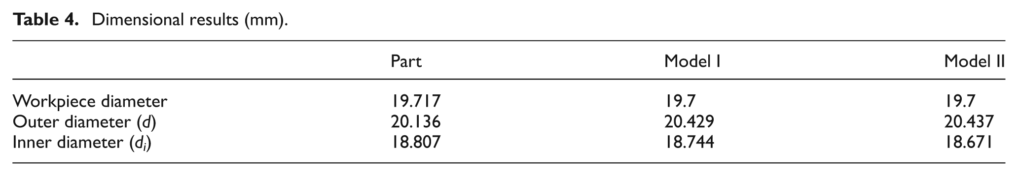
where the proportionality factor, $α$ , is approximately 3. For plastically deformed materials, $σ_{y}$ in equation (14) should be replaced by the current yield stress, $\bar{σ}$ , in order to take into account the strain hardening. In Figure 23, the scaled stress is presented for both numerical models.

Figure 23.

Micro-hardness Vickers (MPa; scaled by equation (14)): (a) Model I and (b) Model II.

For the experimental model, the hardness varies from 2619 to 2736, that is, over an interval of 117 units. The hardness displayed on the side of the teeth for the under-integrated solid element (Model I) is 2450 units and varies from 2500 to 2350, that is, over an interval of 150 units. For Model I, there is a difference of −7.8% in relation to experimental hardness. The results obtained for the fully integrated solid element (Model II) are less conclusive. The hardness varies from 2200 to 1900, that is, over an interval of 300 units. For the fully integrated model, there is a difference of −19.1% in relation to experimental hardness (Table 5).

Table 5.

Micro-hardness results.

Measured	HV	Scaled HV (by 9.81 m/s²)	Numerical model
			Model I (MPa)	Model II (MPa)
1 (bottom)	279	2736	2500	2200
2 (middle)	271	2658	2450	2150
3 (top)	267	2619	2350	1900

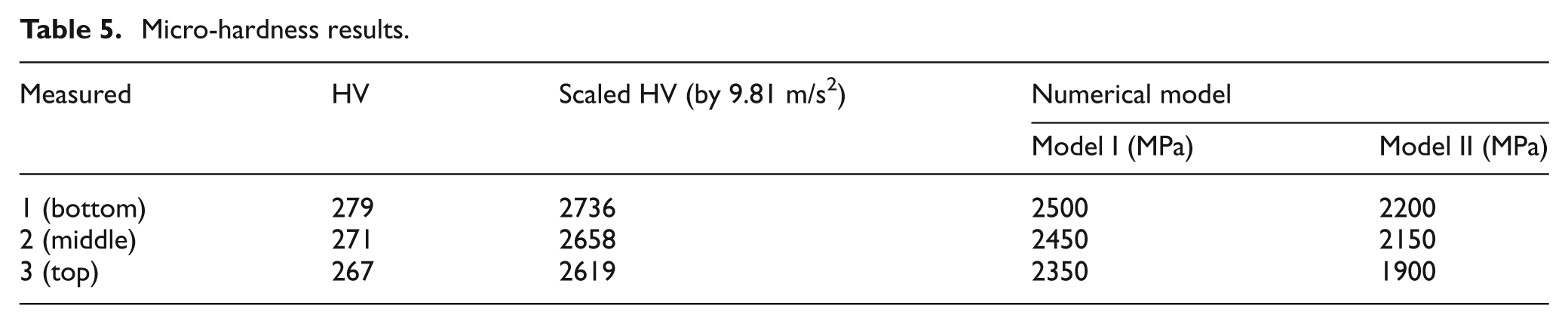
Figure 24 presents the histories of the energies recorded during the numerical simulation. Major differences between the calculated values would have indicated that the numerical models behaved differently during the simulation process.

Figure 24.

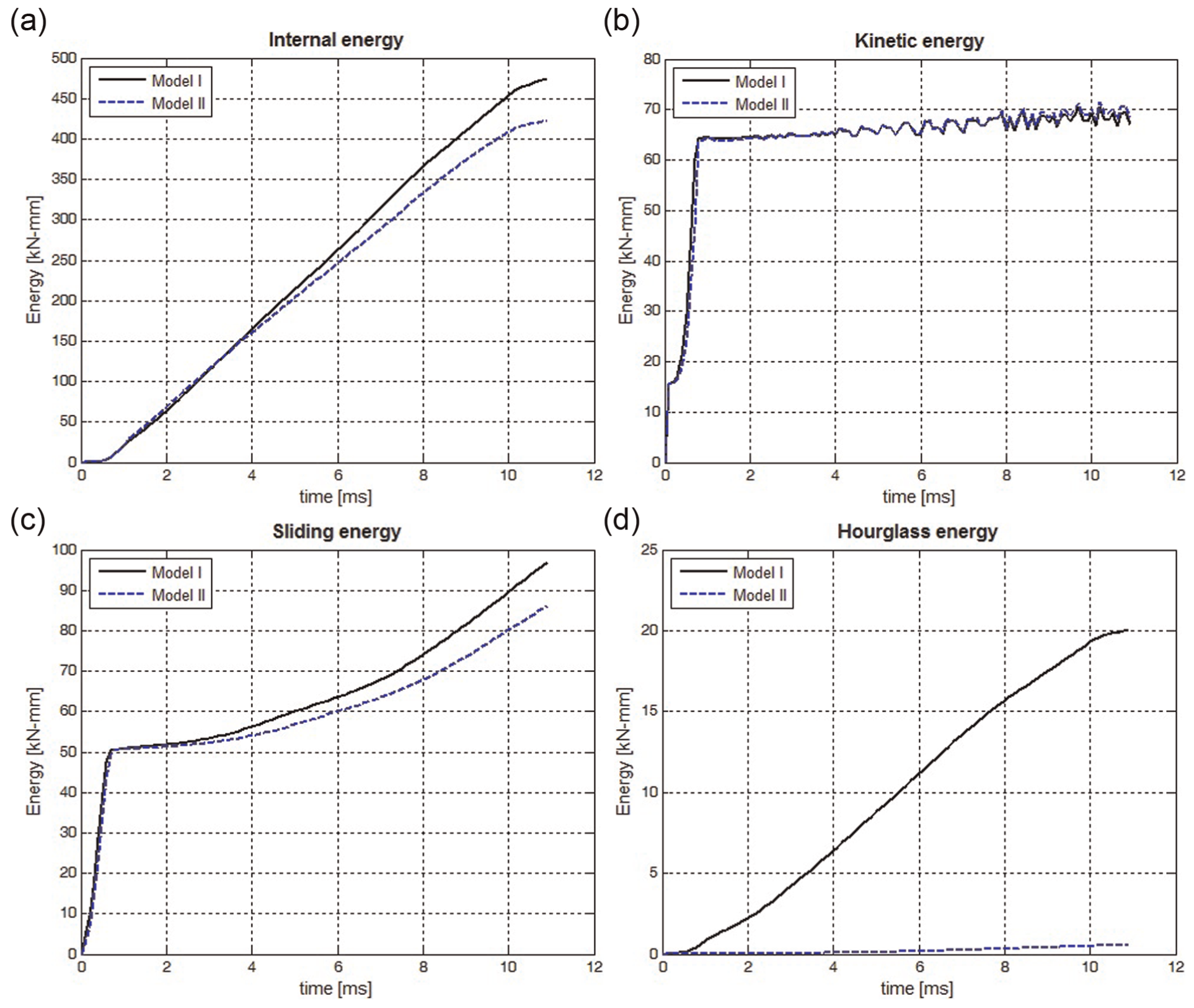
Measured model energies: (a) internal energy, (b) kinetic energy, (c) sliding energy and (d) hourglass energy.

The internal energy consumed during the rolling process is approximately 12% higher for the model with constant stress elements (Model I), and there is a close match between the recorded histories for the kinetic energy. The sliding energy is 12% higher for the model with constant stress elements, yet a noticeable difference between the results is obtained for the hourglass energy, due to the necessity of hourglass stabilisation of the under-integrated solid element. The recorded values of the hourglass energy, as this energy originates from a force applied to the element,¹⁷ can provide an explanation for the recorded differences between the rolling forces (Figures 17 and 24).

Conclusions

In this study, complex profiles with grooves have been formed by wedge tools. A complete experimental system was developed to acquire and analyse the process parameters for these grooves. The methodologies used to record and evaluate the experimental results and the capabilities of the technique were discussed.

The radial (process) force was measured during the manufacturing process, but the experimental equipment provides the necessary background for the measurement of other parameters, such as the tangential force, using the pressure on the hydraulic circuit from the engine to the tool and the tangential velocity of the wedge tool, which are parameters that will be the focus of further work. The experimental tests were extended, and the material used for the workpiece was investigated to identify a valid mechanical model. Additionally, metallographic studies and micro-hardness studies were performed.

Following the experimental results, a complete numerical model of the wedge rolling process has been presented in this study. The rolling process was investigated using both experimental methods and numerical methods (explicit analysis with LS-Dyna).

Finite element simulations of the cold rolling process have been performed using a robust numerical model and an extrapolation of the stress–strain law with the five parameters identified in the compression tests. A number of parameters were investigated to identify the best practise for the wedge rolling analysis: element formulation (fully integrated versus under-integrated element), material model, contact interface and simulation time.

Based on the experimental results and the numerical analysis, to obtain a reliable computational model (to lead to good results to be run in a short time), the following issues should be addressed:

-The material model and material data used for the numerical analysis should be related to a law with multiple parameters;

-The numerical model must be developed with respect to the process definition (contact between parts using null material);

-Adequate use of the forming capabilities of LS-Dyna that will provide the contact interface;

-Identification of the simulation time (method and parameters evaluated). The simulation time can be identified by comparing the transition from stationary to forming process using successive times. It was also found that for the preliminary analyses, only 20% (first workpiece rotation) of the time should be run thus providing a considerable advantage for model set-up.

-The under-integrated finite element with hourglass stabilisation is capable of providing accurate results (dimension and micro-hardness) over the fully integrated element and it has the major benefit of reasonable runtimes.

The numerical model makes it possible to forecast the strain and stress state, evaluate the process forces and anticipate the phenomena limiting the wedge rolling process stability. The model can be used to analyse the influence of several process parameters (e.g. workpiece material, workpiece diameter, wedge slope and wedge translational velocity) on the final part (e.g. dimensions, stress and strain state and micro-hardness).

The present model will be further improved to enable the simulation of various rolling processes for products with more complex shapes and to enhance the integration of the rolling process in computer-aided design (CAD)/computer-aided manufacturing (CAM)/computer-aided engineering (CAE) systems.

Footnotes

Declaration of conflicting interests

The authors declare that there is no conflict of interest.

Funding

This work was supported by CNCSIS – UEFISCDI, project number PN II – IDEI 711 – 2008, ‘Analytical and numerical modelling of the processes of cold plastic processing of complex profiles’.

References

Rowe

Sturges

CEN

Hartley

. Finite-element plasticity and metalforming analysis. Cambridge: Cambridge University Press, 1991.

McCormack

Monaghan

. A finite element analysis of cold forging dies using 2D and 3D models. J Mater Process Tech 2001; 118: 286–292.

Martin

. Fundamental finite element evaluation of a three dimensional rolled thread form: modeling and experimental results. In: Fatigue Fract Resid Stresses, ASME/JSME Joint Pressure Vessels and Piping Conference. San Diego, 26–30 July, 1998; 373: 457–467.

Domblesky

Feng

. Two-dimensional and three-dimensional finite element models of external thread rolling. Proc IMechE, Part B: J Engineering Manufacture 2002; 216: 507–517.

Domblesky

Feng

. A parametric study of process parameters in external thread rolling. J Mater Process Tech 2002; 121: 341–349.

Pater

Gontarz

Weroñski

. New method of thread rolling. J Mater Process Tech 2004; 153–154: 722–728.

Kamouneh

Stephenson

. Diagnosis of involumetric issues in flat rolling of external helical gears through the use of finite-element models. Int J Mach Tool Manu 2007; 47: 1257–1262.

Lee

Yoon

. Optimization of design parameters using a response surface method in cold cross-wedge rolling. J Mater Process Tech 2008; 201: 112–117.

Wang

Fan

. Complete modeling and parameter optimization for virtual ring rolling. Int J Mech Sci 2010; 52: 1325–1333.

10.

Guo

Yang

. Towards a steady forming condition for radial–axial ring rolling. Int J Mech Sci 2011; 53: 286–299.

11.

Niţu

Iordache

Marincei

. FE-modeling of cold rolling by in-feed method of circular grooves. Stroj Vestn: J Mech E 2011; 57: 667–673.

12.

Aghchai

Razani

Mollaei

. Flow forming optimization based on diametral growth using finite element method and response surface methodology. Proc IMechE, Part B: J Engineering Manufacture 2012; 226: 2002–2012.

13.

Hartley

Srinivasan

. Constitutive equations for large plastic deformation of metals. J Eng Mater: T ASME 1983; 105: 162–167.

14.

Johnson

Cook

. A constitutive model and data for metals subjected to large strains, high strain rates and high temperature. In: Proceedings of the 7th international symposium on ballistics, La Haye, The Netherlands, 19–21 April 1983. American Defense Preparedness Association (AFDA): pp.541–547.

15.

Tabor

. The hardness and strength of materials. J I Met 1950; 70: 1–18.

16.

Borrvall

. A heuristic attempt to reduce transverse shear locking in fully integrated hexahedra with poor aspect ratio. In: 7th European LS-DYNA conference, Salzburg, Austria, 14–15 May, 2009.

17.

Hallquist

. LS DYNA theory manual. Livermore, CA: Livermore Software Technology Corporation, 2006.

Finite element analysis and experimental validation of the wedge rolling process