
Abstract
This article examines the relationships between the quality of a machined component and the non-intrusive measurements that can be made during the manufacturing process. For the purposes of this study, the overall quality of a machined component is defined by the surface finish and any residual stress induced by the machining process. The focus of the work involves turning of difficult-to-machine metals and non-intrusive measurements recorded during machining. These measurements were acoustic emission, cutting forces and cutting insert temperature. An austenitic stainless steel was chosen as a commonly available metal whose high work-hardening rate and ability to strain transform to martensite make it potentially difficult to machine. Tests were carried out under different cutting conditions to promote thermally and mechanically induced residual stress and variations in the surface finish. Analysis of the mean frequency of the acoustic emission signal has made it possible to determine whether thermal or mechanical interactions dominate the machining process. The mean frequency of the machined samples provided evidence of a thermally driven process. This was confirmed by the close relationship between cutting insert temperature and component residual stress. The analysis of low-frequency acoustic emission generated during machining (below 100 kHz) identified poor surface finish derived from vibrations of the cutting insert.
Introduction
It is becoming increasingly important for many manufacturing industries to be able to control the quality of the final component. Two key attributes that determine the overall quality of a machined component are residual stress and surface finish, as both can have a significant effect on service life. Although there are numerous techniques for measuring the residual stress in a component, most require the component to be removed from the machine tool and either destructively tested or have energetic particles fired at them. Similarly, it is difficult to assess the surface finish comprehensively without removing the component from the machine tool. For industries manufacturing high-value components, these techniques are often not a viable solution.
The tool–workpiece interaction obviously plays an important role in the generation of the final component surface, both in terms of its finish and any residual stress. For example, if the cutting tool breaks during machining, the resulting surface will be much rougher due to variations in the cutting edge. On the contrary, an excessively blunt cutting edge may fail to penetrate the surface during cutting and produce a smoother surface, although often of poorer quality due to burnishing and pressure welding. A further cause of poor surfaces is from vibrations present during machining. Machine tools inherently have natural vibration frequencies. Any relative vibration of the machine tool, cutting tool or workpiece can be imprinted onto the surface of the component.
A robust technique is therefore desirable to quantify the residual stress and surface finish of a component that is both non-destructive and small enough to use in situ during machining. The aim of the current work is to investigate whether acoustic emission (AE) can be used as an online sensor to provide information about the quality of a turned component as defined by the surface finish and residual stress.
Background
AE is the term used for the generation of elastic waves by rapid changes in the internal stress field of the material. 1 The waves cause surface displacements as they propagate through the material that can be detected using transducers. AE analysis has the distinct advantage that data can be recorded while machining operations are occurring. The signal carries information on processes such as plastic deformation (dislocation movement), crack growth and martensitic phase transformations and so, in principle, is suitable for the application.
Figure 1 depicts a generic AE set-up, which will typically involve one or more (usually lead zirconate titanate (PZT)–based piezoelectric) transducers with associated preamplifiers, which convert a surface disturbance in the nanometre range to a voltage, which can be acquired from a computer. The ‘raw’ signal typically contains frequencies in the 0.1–1 MHz range, and it is common for the preamplifiers to contain an analogue band-pass filter in this range. A number of AE systems exist, many of which provide software for processing the raw signals and extracting various time-, frequency- and time-frequency features. However, the approach taken in this work was to acquire the raw signal in its entirety, and the extract features by digital signal processing, using techniques very similar to those use for acceleration monitoring, except that frequencies are generally higher. 2 In the current work, only two AE features are used, the simplest being the ‘AE energy’, which is essentially the integral of the square of the AE voltage over a fixed record length with a fixed degree of amplification. 3 This energy is not calibrated but gives a relative measure, provided the sensor sensitivity and the amplifier settings are held constant. The other method that is used is to demodulate the AE time series, by batch averaging it. This allows characteristics to be revealed below the signal bandwidth, with the propagating ultrasound acting as a carrier wave. 4 The averaged signal can be cast into the frequency domain using standard signal processing techniques, such as the fast Fourier transform (FFT), and, as in the current case, single features can be extracted from the demodulated (or raw) spectrum such as its mean frequency (first moment of the spectrum).
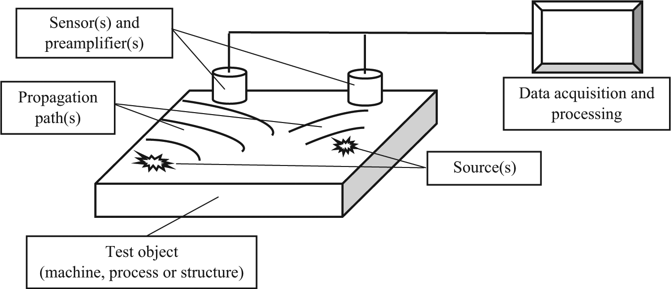
Generic AE set-up for monitoring machines, processes or structures.
There has been a wealth of research into process monitoring during orthogonal single point turning.5,6 General machining theory suggests that increasing the feed rate produces components with worse surface finishes and that altering the depth of cut has no effect. An ideal value for the surface finish (Ra) can be determined by considering only the geometric contribution from the feed rate (f) and cutting nose radius (r), 7 see equation (1). This ideal will, of course, be affected by vibration, tool set and tool wear:

Jang et al.8,9 have observed that increasing both the cutting speed and the feed rate increase the tensile surface residual stress of turned austenitic stainless steel bar and attributed the erratic effect of depth of cut to variable pre-existing residual stresses. Outeiro et al. 10 found that increasing the feed rate led to increased residual stresses in turned austenitic stainless steel, whereas increasing the depth of cut produced a reduction in the residual stress. Using a selection of steel grades with varying mechanical properties, Capello 11 found that the main variables that affect the residual stress of a component were feed rate and tool nose radius, and that the depth of cut had no effect. Finally, M’Saoubi et al. 12 reported increased residual stresses of orthogonally machined stainless steel components with increased cutting speed and feed rate.
The use of AE for machining process monitoring has been studied for several decades,13–16 the majority of the research being focused on the relationship between tool wear and AE generated during machining. Significantly less has been done on the effect of machining parameters on the AE signal and the consequent effects on workpiece quality. Rangwala and Dornfeld17,18 investigated the relationship between the energy and the spectral content of AE recorded during orthogonal turning of tubular 6061-T6 aluminium alloy components and the cutting conditions. They suggested that a decrease in dislocation mean free path or increase in dislocation velocity would shift the AE signal power to higher frequencies. Plastic deformation of highly strain hardened material is expected to decrease the mean free path due to the large numbers of dislocation forests and sessile dislocations that obstruct the movement of mobile dislocations. Whereas it is unlikely that the speed of dislocation movement would be affected by strain rate, an increased strain and strain rate would certainly result in a higher frequency of arrival of dislocations at obstacles. Competing against these two mechanisms was thermal softening effects, which would increase the dislocation mean free path, hence reduce the dislocation arrival rate at obstacles and shift the spectra towards lower frequencies. Therefore, a maximum mean frequency of the AE spectrum might be expected, above which the thermal softening effects begin to dominate the mechanical effects. In the aluminium alloy studied by Rangwala and Dornfeld, this occurred at a cutting speed of approximately 1 m/s. Araújo et al., 19 working with carbon steels, also found that the mean AE frequency increased with the increasing strain rate and decreased with the increasing temperature. This small collection of work contains a very important observation, as it relates the cutting temperature and plastic deformation, both mechanisms of residual stress formation during machining, to a measure of the AE signal.
Diniz et al. 7 attempted to link the AE energy (measured as the root mean square (RMS)) generated during machining to the surface finish of the final component but did not find any correlation. In addition, Beggan et al., 20 working with diameter turned leaded mild steel bar, observed that, while the RMS AE was highly dependent on cutting speed, Ra values were influenced more by the feed rate, and so a direct correlation between AE and Ra was not established. They did report, however, that the percentage deviation between the measured and the modelled RMS AE, and the Ra showed similar dependences on cutting conditions and hence this deviation in the RMS AE could be used to predict Ra values. This article shows that there is some promise for the use of AE as a method of predicting surface finish, perhaps using some features other than RMS.
Experiment
The basic experimental rationale was to carry out a set of machining tests under various cutting conditions while monitoring the AE in-process and making ancillary measurements of force (three axes) and tool tip temperature. Each test consisted of a facing operation (Figure 2) on a thick stainless steel disc and, after facing, the surface of the disc was assessed for surface quality.
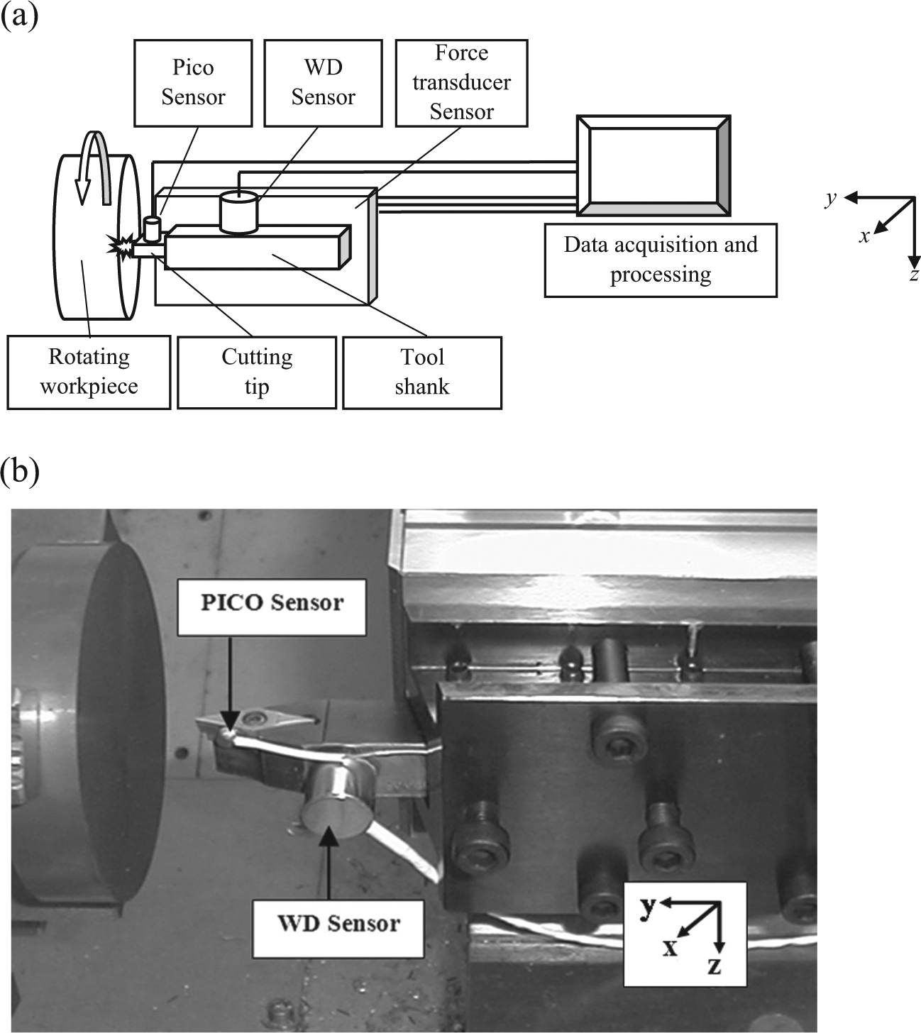
Machining set-up: (a) schematic and (b) photographic, showing the positions of both AE sensors and directions of orthogonal cutting forces, where x is the feed direction, y is the tool axial direction and z is the tool vertical direction.
The stock material was a low-carbon austenitic stainless steel (304L), supplied as 50-mm diameter round bar, and was cut into 25-mm discs to make each sample. The samples were faced after cutting and were each stress relieved at 1050 °C for 1 h followed by cooling at a rate of 100 °C per hour. Once prepared, the specimens were then mounted in the chuck of a Dean Smith and Grace CNC MT2410 ‘Pony’ lathe. A fixed spindle speed of 500 r/min was used for the facing operation, giving cutting speeds that varied between 160 m/min and 0 between the outer diameter and the centre of the bar. Three feed rates, 25, 50 and 100 mm/min, were used and depths of cut varied between 0.05 and 2 mm, so that a total of 38 different cutting conditions were used, giving a range in material removal rate (MRR) of between about 400 and 47,000 mm3/min, a similar range to that used by Rangwala and Dornfeld. 18
Two wideband piezoceramic sensors (Physical Acoustics type wideband differential (WD) and PICO) were used to record the AE. Both sensors respond in the range 0.1–1 MHz, and both were equipped with preamplifiers containing analogue filters over this range. The WD sensor is about 5 dB more sensitive than the PICO sensor, but the latter is small enough that it could be mounted directly onto the tool tip, thus avoiding potential transmission losses along the shank and across the tip–shank interface. In addition to recording the AE, a three-axis Kistler dynamometer was used to record the cutting forces, and an infrared pyrometer was used to monitor the bulk cutting insert temperature. The experimental set-up is shown in Figure 2. AE was recorded at full bandwidth across the whole cut in each sample, synchronously with the cutting forces and cutting insert temperature. This meant that, although the forces and the temperature were considerably over-sampled, the entire record could be indexed with the post-machining quality indicators.
After machining, the quality of the turned components was assessed by measuring the surface finish, residual stress, hardness and determining the sub-surface microstructure. The surface finish was measured using two-dimensional and three-dimensional scanning with a Form Talysurf stylus profilometer. Subsequently, the hardness of the machined surface was measured using a Vickers hardness indenter. Following these measurements, a hole drilling technique was used to quantify the manufacturing stresses on the machined surface. Rosette strain gauges were bonded to the surface of the component through which a high-speed turbine drill incrementally machined a small diameter hole. Metallurgical sections were prepared to investigate the extent to which residual stresses were caused by martensitic transformation using optical microscopy and electron backscattered detection (EBSD). All of the quality indicators were recorded at a range of diametral positions on the machined surface, so that they could be identified with the AE and other in-process measurements.
Results and discussion
The raw recorded AE for each sensor consisted of between 30 s and 2 min of data sampled at 2 MS/s per sensor. A suite of codes was especially written in the LabVIEW environment to determine the frequency content of the AE signal and also calculate the mean frequency of the raw AE, the RMS at a variety of averaging times and the AE energy.
Figures 3 and 4 show typical output screens from the software suite, illustrating how the main AE features were derived. Figure 3 is the output from a typical 1-s batch of raw AE, used to obtain spatially localised values of AE energy and mean frequency. The 1-s batch is a compromise between giving sufficient time to obtain the features but not so much time that the cutting speed varies significantly. Figure 4 shows a longer (15-s) segment of AE, used to form a demodulated spectrum that reveals frequencies below the sensor bandwidth. As can be seen, the amplitude of the raw AE record declines gradually over the 15 s, a consequence of the reducing cutting speed as the tool moves towards the centre of the workpiece. As can also be seen, the demodulated spectrum contains ‘system’ peaks that do not vary with cutting conditions as well as motile peaks that change in frequency as the cutting conditions change.
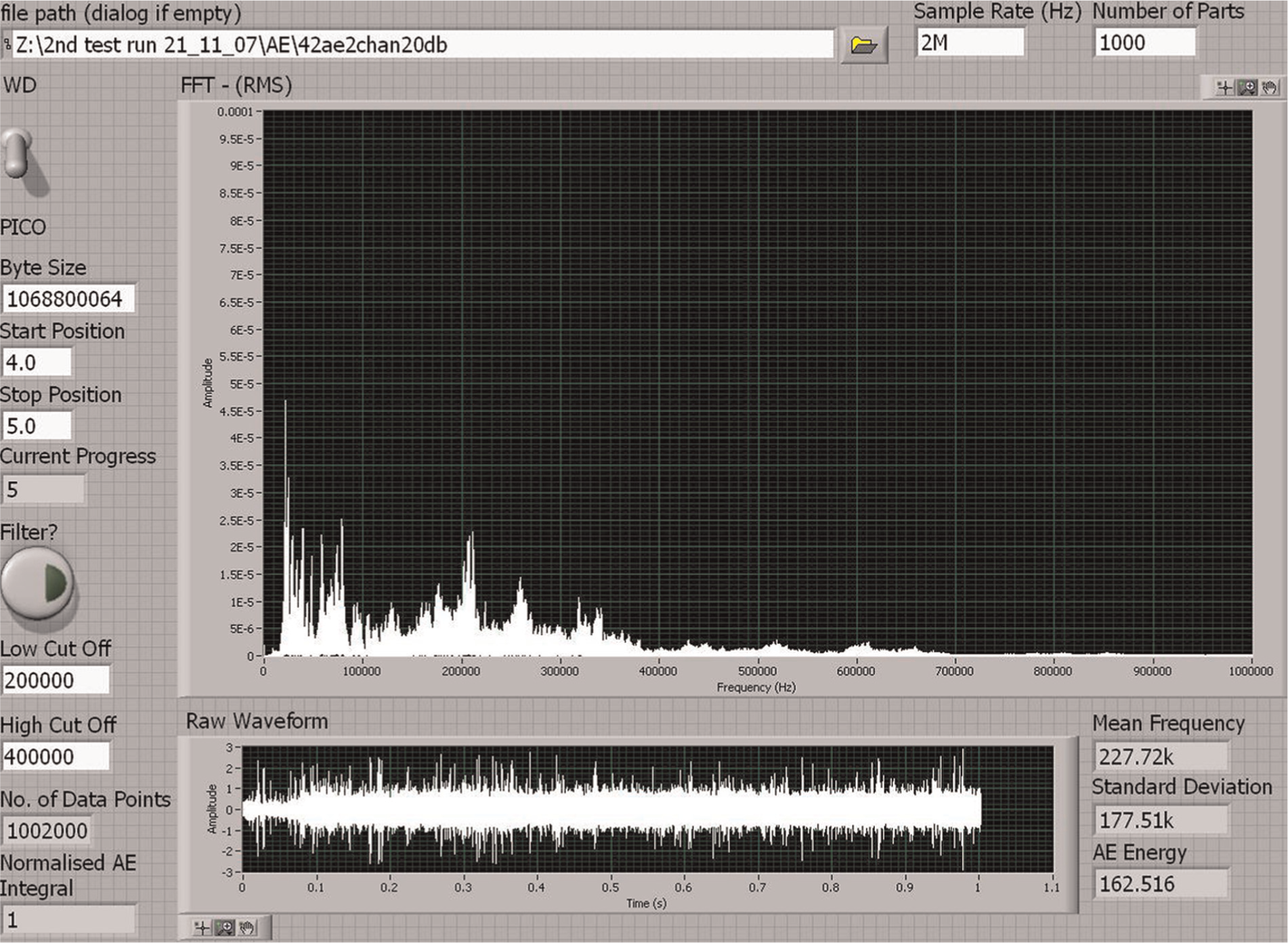
Sample output screen of typical 1-s batch of raw AE recorded with the PICO sensor. Bottom trace shows the raw record and the top trace shows the power spectrum.
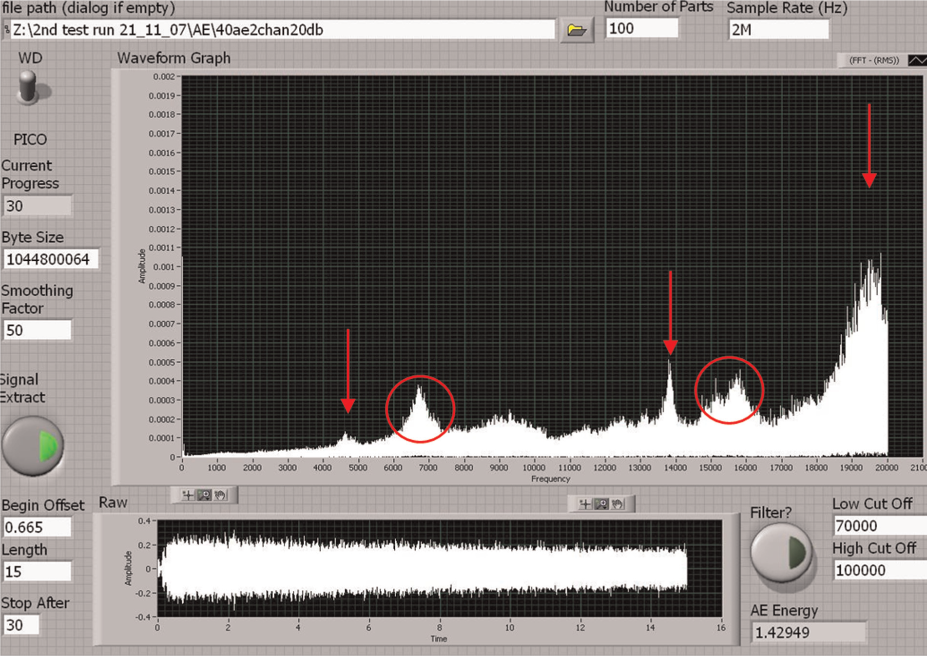
Typical 15-s record of AE averaged over 50 points from the raw record recorded by the WD sensor. Bottom trace shows the raw signal (before averaging) and the top trace shows part of the demodulated spectrum.
The analysis of online processing data and post-machining component quality results has established the following relationships.
AE mean frequency variation with cutting speed
Figure 5 illustrates the variation of cutting speed with AE mean frequency measured using the WD sensor. The data come from three specimens that were all machined with the same depth of cut over a range of feed rates. Two-second segments of the raw AE data were extracted from each sample record, each segment being assigned an average cutting speed. The segments were each analysed for mean frequency, giving results over a range of cutting speed to compare with the data of Rangwala and Dornfeld 18 for orthogonal turning of aluminium. The data presented here are a small subset of the study, although the remaining datasets, using different depths of cut recorded by both the PICO and WD sensor, showed very similar results.
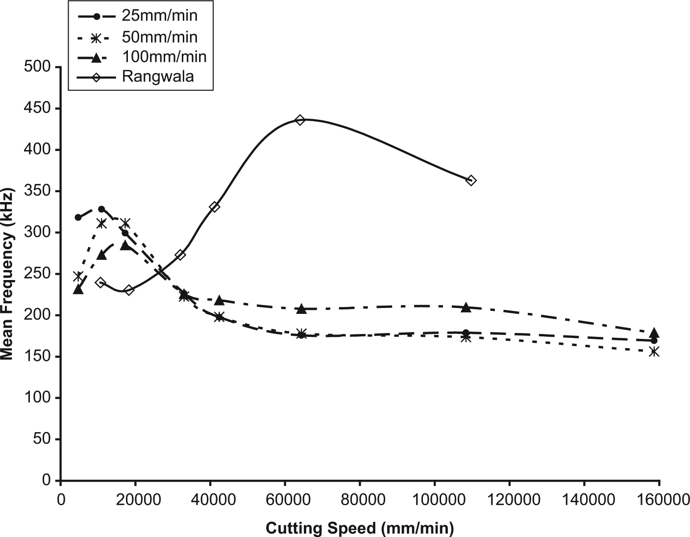
Variation of AE mean frequency with cutting speed at different feed rates compared with published data. 17
As mentioned earlier, Rangwala and Dornfeld 18 attributed the peak at a cutting speed of about 70 m/min to the point at which the effect of thermal softening overcomes the strain hardening. The aluminium alloy studied by Rangwala and Dornfeld has a lower thermal softening temperature and a higher thermal conductivity than the stainless steel in the current work. Despite this, the results from machining stainless steel demonstrate a very similar trend except that the critical cutting speed is around 20 m/min and is independent of depth of cut or feed rate (from examination of the full dataset). The difference can be explained by the lower work-hardening rate of aluminium alloys (affecting the mean cutting stress at a given temperature, thus reducing the work done at a given MRR) and the greater thermal conductivity of aluminium (leading to faster heat dissipation for a given heat input). These effects could also explain why the peak mean frequency is lower in stainless steels than it is in aluminium. The cutting speed of 20 m/min occurred when the insert was very close to the centre of the stainless steel component, after 95% of the machining operation had been completed. Thus, for the vast majority of the machining operation, the data suggest that thermal effects were dominating over mechanical effects and hence all of the residual stress and hardness measurements were recorded in areas of the specimen that were thermally driven. It is not surprising, then, that metallurgical and e-beam back-scatter analysis found no evidence of martensitic phase transformation. The dominance of thermal effects is in agreement with conclusions formed by Sharman et al. 21 when machining Inconel. It is also interesting to note that Outeiro et al. 10 did not observe martensitic phase changes with a similar machining operation on a similar material.
Residual stress, temperature and hardness variation with MRR
The variation of cutting temperature measured at the insert and machined surface hardness with MRR can be seen in Figure 6.
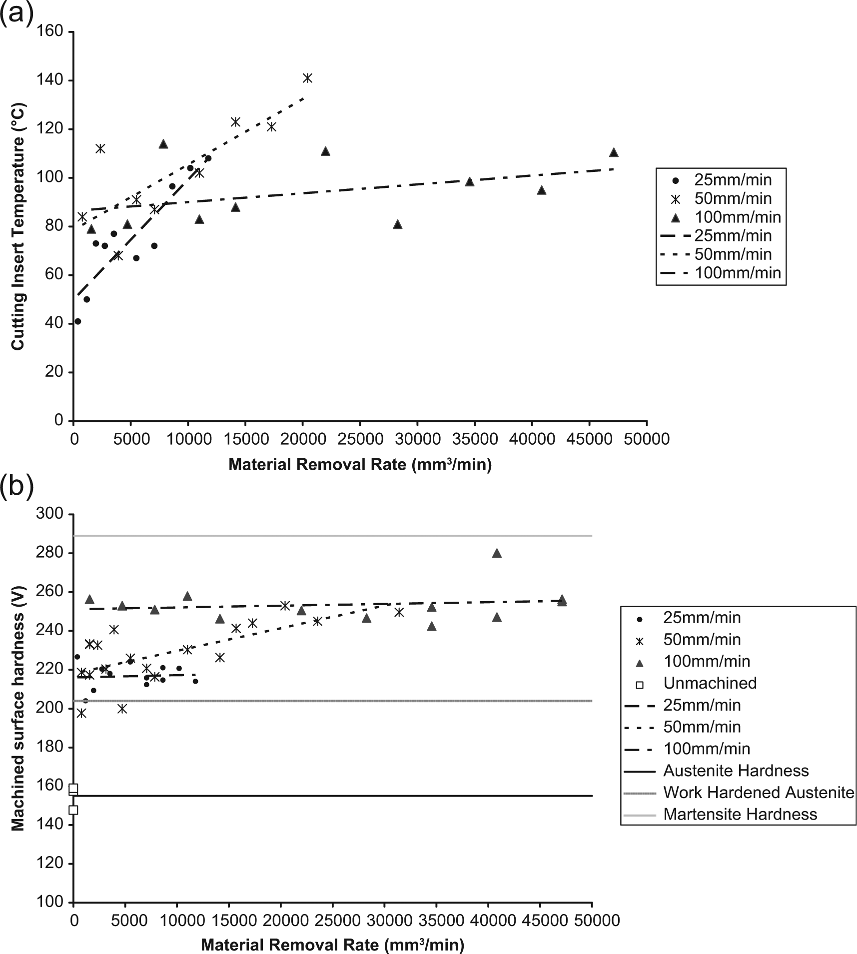
Effect of material removal rate on (a) cutting insert temperature and (b) machined surface hardness.
The cutting insert temperature generally increases with MRR, although the rate of increase decreases with the increasing feed rate. M’Saoubi et al. 12 suggested that increasing the cutting speed increases the chip flow rate and consequently leads to greater heat dissipation through the chips, although it is not clear why this would be proportionately greater than any other dissipation mechanism, such as the increased surface area provided for conduction into workpiece and chip offered by an increased depth of cut. Since increased cutting speed increases the deformation rate, whereas the other two cutting conditions, depth of cut and feed rate, increase the cutting force (at a given temperature and strain rate, hence stress), it seems more likely that the data suggest that strain rate has a larger effect on the energy input to the workpiece and tool. The temperature of the tool tip might be expected to be proportional to the product of cutting force and cutting speed and the disproportionate effect of cutting speed can be attributed to its affecting the cutting force through work hardening.
The variation of hardness with MRR shows a weaker, but similar, trend in that the lower feed rates have a greater tendency to increase with MRR than the highest feed rate. The trend for the variation between residual stress and MRR reflects that for hardness, where an increase with MRR is evident for the 50 mm/min feed rate, whereas it varies little for the 100 mm/min feed rate. The variation is also very weak for the 25mm/min feed rate although the range in MRR at this feed rate is much smaller. As mentioned previously, there is some debate in the literature as to the effect of depth of cut on the final component residual stress. This probably means that residual stress varies with a combination of factors. The work being put into the cutting process is the product of cutting force and cutting speed. The cutting force will increase with the cross-sectional area of the undeformed chip (proportional to product of depth of cut and feed rate) but will also decrease with temperature at the cutting site and may also increase with cutting speed.
To help illustrate the remarkable similarity between the relationships involving residual stress and cutting temperature, Figure 7 shows the data plotted on the same graph along with some data gleaned from the literature. Figure 7 adds further evidence that thermal effects are dominating the machining process or at least that both evolutions are driven by the same factors.
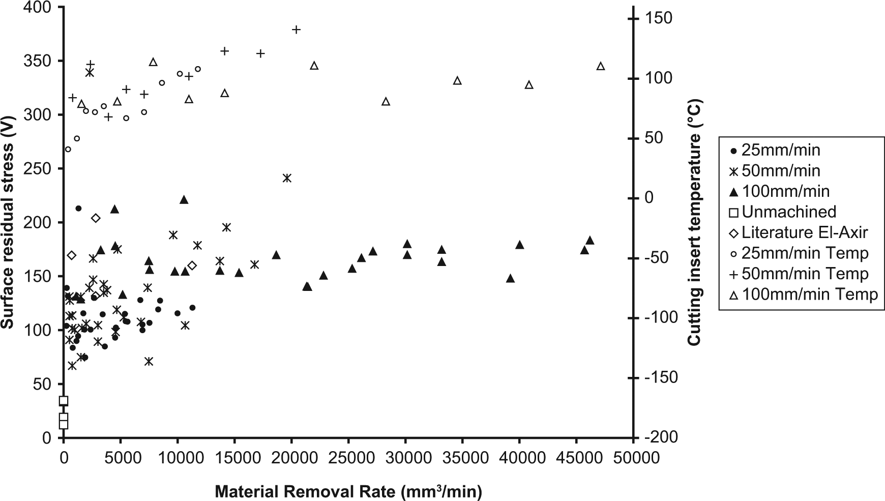
Effect of material removal rate on cutting insert temperature and post-machining surface residual stress at various feed rates (including data from El-Axir 22 ).
The cutting insert temperature provides a reasonably direct measure of the thermal energy introduced into the material. Since the residual stress of the component follows the cutting insert temperature, it can therefore be inferred that the thermal energy introduced into the component is the primary cause of the final residual stress state, rather than the degree of plastic deformation at the surface, which would increase with MRR in an approximately linear fashion. The thermal energy that is put into the component softens the plastic zone that surrounds the cutting point and reduces the amount of sub-surface work hardening. This has been confirmed by hardness measurements and also metallography.
The process for obtaining residual stress data using the hole drilling technique has many potential sources of error. These include local strain variations on the surface of the material, the bond between strain gauge and specimen surface and the condition of the joint between wires and strain gauge. To assess this variability, several of the specimens had multiple readings taken, and in an attempt to mitigate it, a large number of specimens were machined producing a large dataset. El-Axir 22 and M’Saoubi et al. 12 have also presented residual stress measurements for orthogonally machined 316L stainless steel. Figures 7 and 8 show these literature data points plotted next to the experimental data.
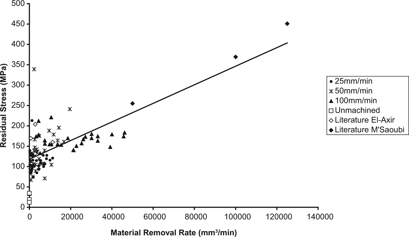
Figure 8 highlights the very high MRRs of M’Saoubi et al. compared with this work and with El-Axir. The combined data are reasonably consistent and illustrate that low MRRs (those of most interest in finishing operations) generally produce lower and more scattered patterns of residual stress, perhaps because they result in more variation in thermal conditions as a result of erratic chip departures. Whether or not the scatter in residual stress within the cutting conditions investigated here is real or is an artefact of the measurement, it is more fruitful to seek a relationship between the online measurements and MRR than directly with measured residual stress.
Cutting forces and AE energy
A preliminary examination of the cutting force data indicated that the feed (normal) force was more sensitive to MRR than were the other two components, and so this article focuses on the feed force. Figure 9 shows how the feed cutting force and AE energy vary with MRR.
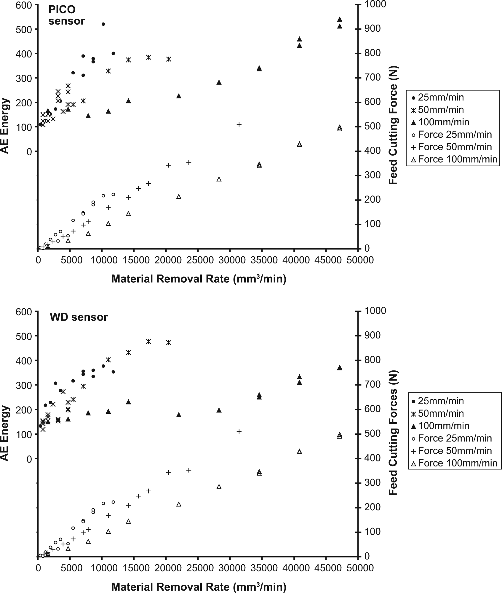
Effect of material removal rate on feed cutting force and AE recorded by PICO sensor (top) and WD sensor (bottom) at various feed rates.
The AE energy measured by both the PICO and the WD sensors shows the same response to cutting conditions as does the feed cutting force. The slope of the feed cutting force and also the AE energy against MRR decreases with the increasing feed rate, an observation that is reflected in the evolutions of all of the quality indicators (hardness, residual stress and tool temperature). This further confirms that cutting speed has an effect on quality out of proportion to its effect on the strain rate, again reinforcing the suggestion that the higher strain rate increases the flow stress of the stainless steel. The direct link between AE and feed force, coupled with the similar evolutions of both online parameters and workpiece quality indicators, shows that there is a good prospect of using either online measurement to monitor workpiece quality. Since AE is easier to measure than cutting forces, the prospect looks good for AE as a monitor for workpiece residual stress, notwithstanding the fact that the variations in measured residual stress in this work are relatively small and scattered.
Component surface finish correlation with AE
The three-dimensional contour profilometer maps showed some non-kinematic periodic information that had been machined into the component, presumably as a result of forced vibrations during cutting. This information is visible as crenulations in Figure 10(a), and as more sophisticated patterns in both the circumferential and radial directions, as seen in Figure 10(b). In order to obtain spatial frequencies that can be identified with temporal frequencies, two-dimensional profiles of the surface finish along the spiral machining grooves (illustrated in Figure 10(b) by the black lines) were extracted from the three-dimensional measurements using inbuilt profilometer software (Talymap). These two-dimensional surface profiles were then analysed using an FFT algorithm and, as shown in Figure 11, the resulting spectra contained a distinctive peak at a spatial frequency equivalent to 4.5 kHz, whose height showed a good correlation with MRR.
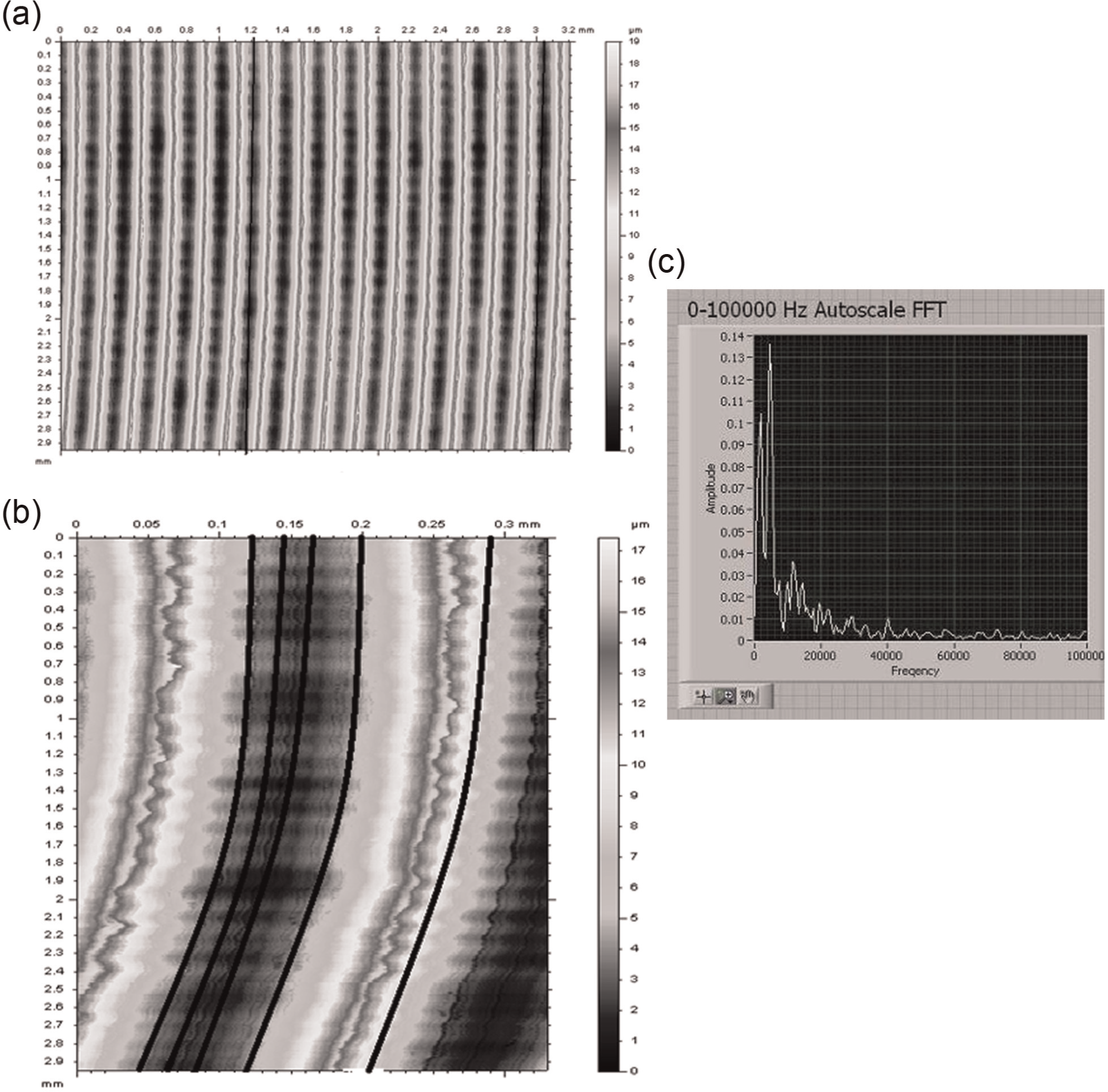
Three-dimensional surface finish data of a machined component at different magnifications: (a) 3.2 × 2.9 mm, (b) 0.32 × 2.9 mm, showing one complete machining groove along which several two-dimensional profiles were extracted, and (c) normalised spatial frequency.
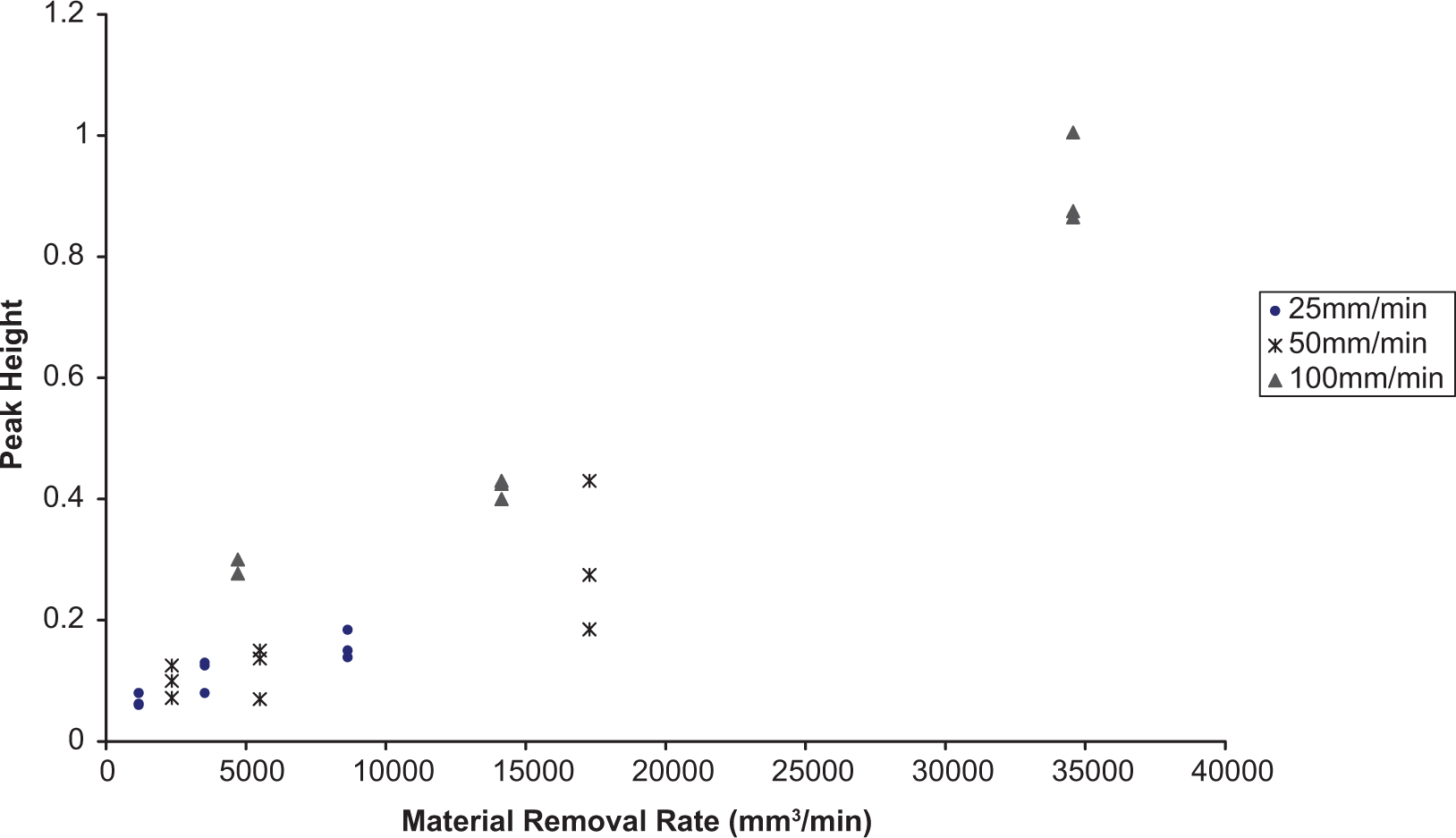
Effect of material removal rate on surface finish spectral peak height at a spatial frequency equivalent to 4.5 kHz.
Separate analysis of the demodulated AE recorded during machining at the same region in the record (located from the position of the analysed surface profile and the known feed rate) was carried out. The raw AE signal was first averaged digitally with an averaging time sufficient to reduce the effective sampling rate to one that would reveal demodulated frequencies in 10-kHz region. The averaged time series was then passed through an FFT algorithm, and the heights of the resulting major frequency peaks were recorded. A correlation between the AE spectral peak heights at 4.5 kHz and MRR was again observed, as can be seen in Figure 12. The above analysis is rather laborious, since the surface profile instrument does not operate online and the two records had to be manually matched. However, the results are sufficiently promising to suggest that demodulated AE could be used as an online indicator of the force pulsations that give rise to the non-kinematic patterns in the machined surface.
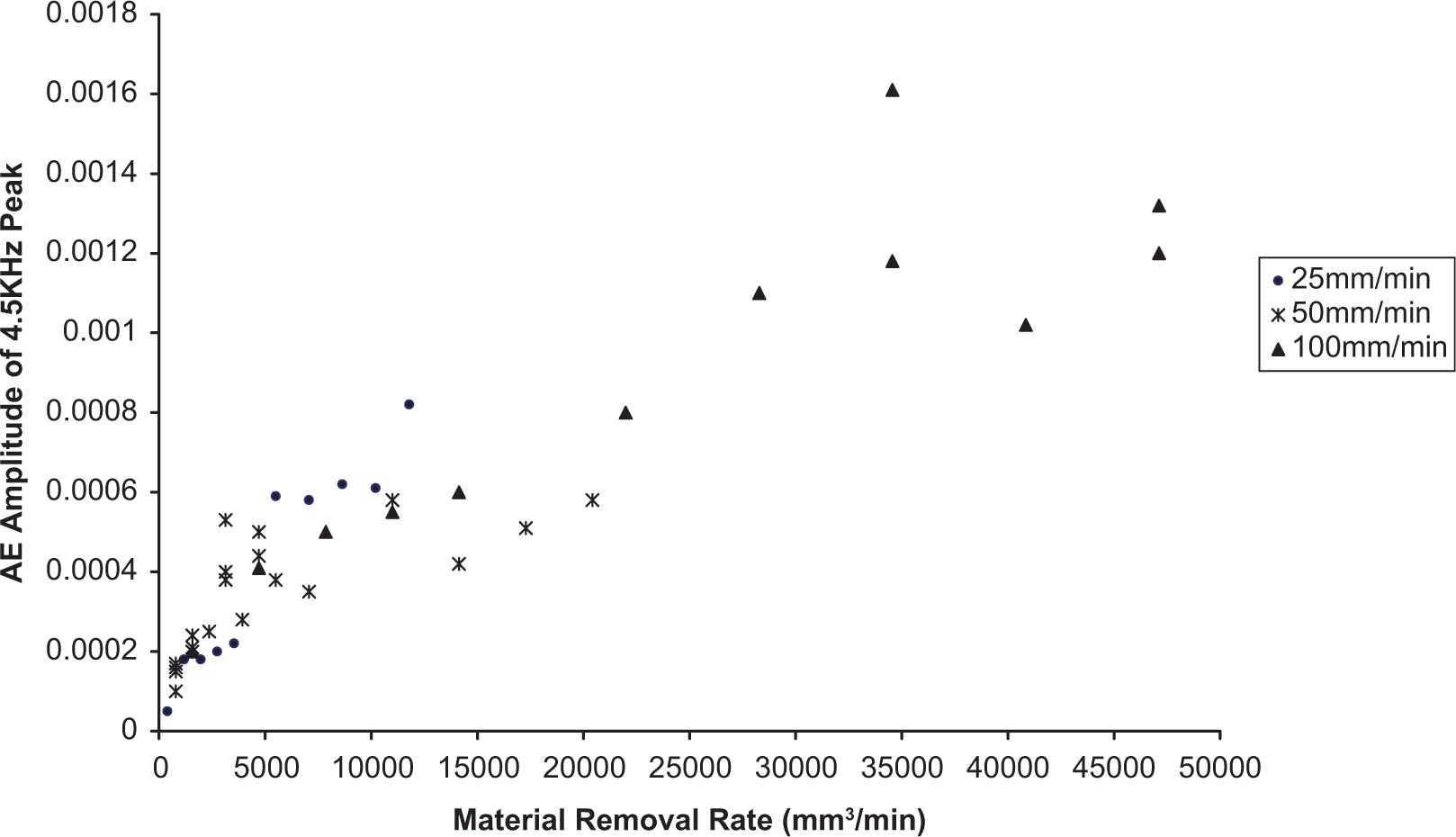
Effect of material removal rate on demodulated AE spectral peak height at 4.5 kHz.
Conclusions
In the course of this work, a number of conclusions were formed about the inter-relationship between the primary offline measures of component quality, residual stress and surface finish; the secondary online and offline assessments of quality, including tool temperature, hardness and metallographic structure and the primary and secondary measurements, AE and cutting force. These are covered elsewhere, 23 and the following conclusions are confined to those directly about the relationship between AE and component quality.
Demodulated resonance analysis of the AE signal shows excellent promise as a means of assessing the degree to which tool vibration affects the finished surface profile. It appears that vibration of the tool relative to the workpiece modulates the steady AE generated during the continuous process of cutting. Frequencies corresponding to the non-kinematic features within the tool groove are clearly present in the demodulated AE spectra giving harmonic series similar to those generated by pulse trains. With some development of the techniques and appropriate calibration, the demodulated AE ought to be able to predict the deviation from the theoretical Ra generated by an imprint of a rigid tool, that is, the non-kinematic patterns referred to in ‘Component surface finish correlation with AE’.
Similarities between the AE energy and cutting forces experienced during machining suggest that AE energy is a useful surrogate for cutting force avoiding the need for a force transducer, which inevitably introduced compliance. This, supplemented with the information on mean frequency, could yield information on the thermo-mechanical conditions at the cutting tip.
While it was possible to link the cutting forces and the AE to MRR and mechanical energy input rate, it did not prove possible to demonstrate that AE could be used to monitor residual stress. The reason for this lies partly in the degree to which this aspect of quality could be measured in this work, and partly in the generally low levels of residual stress encountered in these finishing operations. Scattered, low levels of residual stress have also been reported by other workers using the same material under finishing conditions (El-Axir 22 ).
Footnotes
Declaration of conflicting interests
The authors declare that there is no conflict of interest.
Funding
This work was funded by the Engineering Doctorate Centre at Heriot-Watt University, under the Engineering and Physical Sciences Research Council, UK, and also AWE plc, UK.