Sage Journals: Discover world-class research

Abstract

Tolerance analysis has been the topic of many research publications in the recent past. It is a method to evaluate the quality of products in terms of functional tolerances. Most of the assessment procedures in process planning are based on trial-and-error runs, which are costly and time consuming. There is also a distinct lack of research focus in the area of process plan verification in which input variables are generated from experiments. This article first provides an overview of tolerance analysis. The limits of the previous studies are explored. A method to overcome problems in manufacturing tolerance analysis is then proposed. This method is based on the model of manufactured part and deviation domains to obtain mathematical formulations. These formulations are applied to manufacturing tolerance analyses in which experimental data are used as input variables. The results obtained are then used to verify process plans relative to functional tolerances or to identify achievable functional tolerances taking into account a given process plan and a given number of parts per million. A summary of the method used to obtain the experimental data is presented.

Keywords

Tolerance analysis process plan model of manufactured part functional tolerance experimental data

Introduction and literature review

An essential step in manufacturing is to evaluate the quality of products in terms of functional tolerances. During manufacturing, a product can pass through one or several processes, machine tools, fixtures, cutting tools, and the sequence of operations making up the process plan. Consequently, assessing a process plan in terms of functional tolerance is a distinct step in product quality control, also known as tolerance analysis/stack-up. In other words, controlling the quality of products involves verifying whether the design tolerance requirements meet a given process plan.

Tolerance analysis is commonly called tolerance stack-up because dimensions and their tolerances are added together; they are “stacked up” to provide the total possible variation. Geometrical deviations stack up in both the manufacturing process and the assembly process. Thus, tolerance analysis can be divided into two categories: tolerance analysis in assembly^1–2 and tolerance analysis in manufacturing.

Simulation tools for tolerance analysis and dimensional chains are usually unidirectional, for example, dimensional chains in manufacturing (e.g. Δl method presented in the study of Bourdet³). These simulation tools do not take into account small angular deviations between different machining setups because they are projected on to a reference system. This is why three-dimensional (3D) models have recently been developed for more accurate tolerance analysis.

Different approaches have been designed to analyze how geometric tolerances are propagated in 3D space, referred to as 3D tolerance propagation. Most research work on 3D tolerance propagation is based on kinematic formulations, the small displacement torsor (SDT) concept,⁴ matrix representations, and vectorial tolerancing. There are two related steps in 3D tolerance propagation analysis: the representation of the tolerance zone and the spatial tolerance propagation mechanism. To represent tolerance zones in 3D tolerance propagation, Rivest et al.⁵ present a model based on kinematic formulation. The description of the tolerance zone is summarized within the kinematic structure. Similarly, Laperrière and Lafond⁶ propose a kinematic chain model associating a set of six virtual joints with every pair of functional elements in a tolerance chain. The six virtual joints include three small translations and three small rotations. Jacobian transforms are also used in the study of Laperrière and ElMaraghy⁷ for modeling the propagation of small dispersions along the tolerance chain.

Several mathematical tools are used in tolerance analysis: the theory of matrices,^8,9 the vector,^10–12 the SDT concept,^13,14 and another tolerancing model based on the SDT concept, namely, proportioned assembly clearance volume (PACV), developed by Teissandier et al.¹⁵ Most of this research has focused on tolerance analysis in assembly. However, simulating tolerance analysis in manufacturing is also of great interest. Much research work on error propagation in a multistage machining process has been conducted, but very little has been done on process plan evaluation.

Various error propagation analyses in a multistage machining process have been conducted based on the state space model.^16,17 The state space model is a different form of the standard kinematic analysis model. It provides analytical tools for system evaluation and synthesis. The basic task solved in the state space model environment is an estimation of unobserved states based on observed values. Huang et al.¹⁶ use a state space model to describe part error propagation in multistage machining processes. In this model, part quality is affected not only by the machining operation but also by the setup operation. The induced part errors are propagated into the subsequent stage. Thus, the part deviation for each operation includes the datum errors, fixture errors, and machine tool errors. Here, the error propagation model is expressed by a state vector x(k). Zhou et al.¹⁸ use the differential motion vector (DMV) as the state vector to represent the geometric deviation of the workpiece. DMV is an approach whereby the orientation vector is based on the three Euler rotating angles instead of using a unit direction vector.

The above models are limited to an orthogonal 3-2-1 fixture layout. Loose et al.¹⁹ develop a linear model to describe the dimensional variation propagation of machining processes through kinematic analysis of the relationships among fixture errors, datum errors, machine geometric errors, and the dimensional quality of the product. This model can handle general fixture layouts. However, locating errors are based on a temporary contact and this is not practical for a fixture with a plane–plane or cylinder–cylinder contact.

Taking the above limitations into account, Villeneuve et al.²⁰ apply the SDT concept for error stack-up analysis to machining. Following on from this, Vignat and Villeneuve apply the approach to a turning operation²¹ and then more globally to the machining process using the model of manufactured part (MMP) concept.²² The MMP is then included in simulation to verify the defects generated by a process compared with the indicated tolerances.²³ However, in this research, the use of simulations to evaluate a process plan is based on theoretical assumptions about manufacturing defects. This article presents a new method for manufacturing tolerance analysis in which experimental data are used instead.

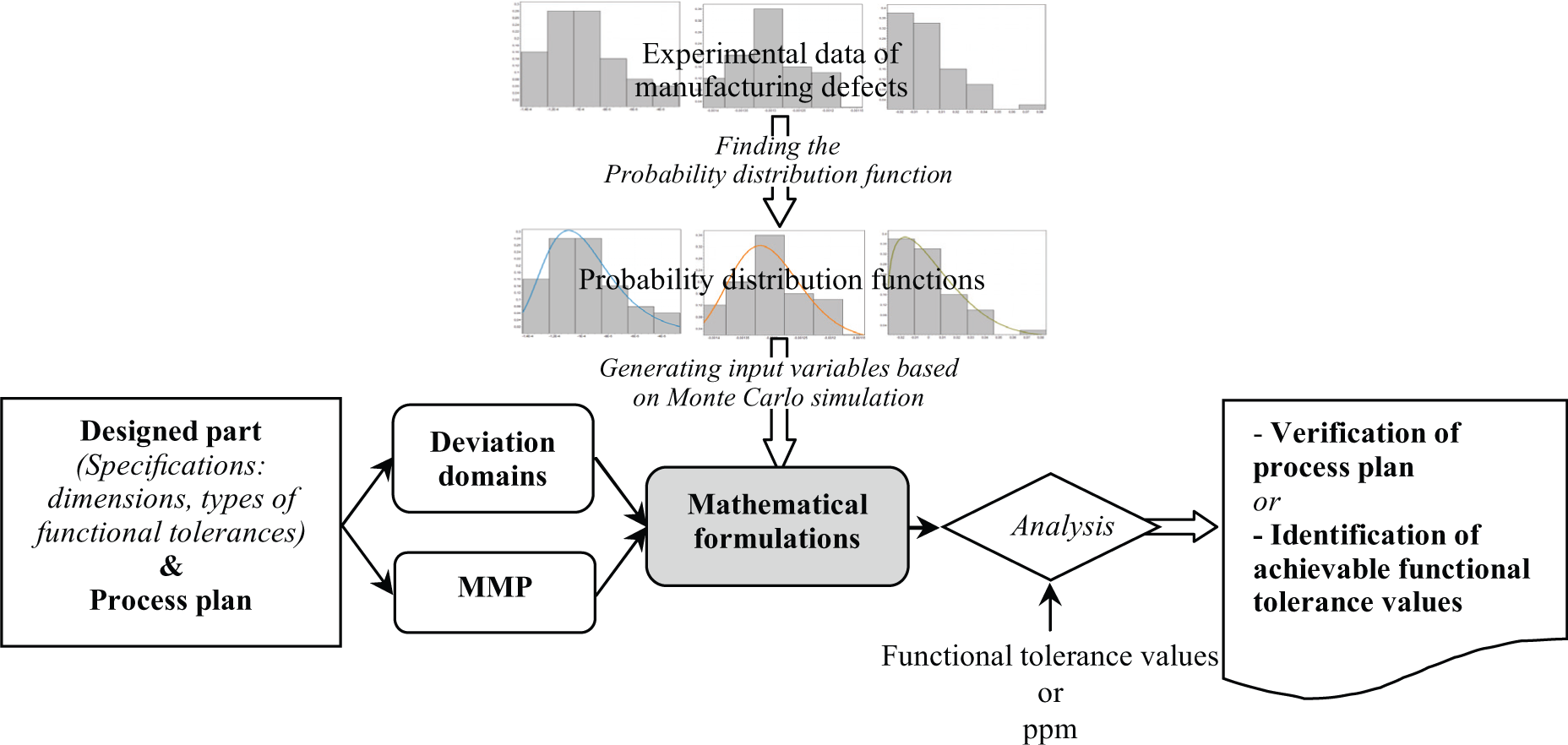
Figure 1 summarizes this new approach. For a given designed part, the deviation domains of each machined surface are built from the type of functional tolerance attached to the surface. The given process plan is modeled using the MMP method. The mathematical formulations rely on the parameters of the MMP and the deviation domains. Experimental data relating to manufacturing defects are identified as probability distribution functions (PDFs). A Monte Carlo simulation driven by PDFs gives input variables for tolerance analysis. If the functional tolerance values are known, then the process plan can be verified. If the parts per million (ppm) value is given, the achievable functional tolerance values can be identified (in the quality control context, “parts per million” is usually abbreviated as “ppm” that means out of a million).

Figure 1.

Tolerance analysis based on experimental data.

The MMP method that models the deviations of machined surfaces as SDT components is described in the section “Overview of the MMP.”“Creating a deviation domain from a functional tolerance type” section outlines how to create a deviation domain from a type of functional tolerance. An overview of the method to obtain the manufacturing defect experimental data and the PDFs is presented in the section “Experimental manufacturing defects.” In the section “Tolerance analysis method: a case study,” a case study is described. The aim is to verify a process plan (for which the functional tolerances values are known) or to identify the achievable functional tolerance values (for which the ppm value is given).

Overview of the MMP

Villeneuve and Vignat²⁴ propose a method for modeling the geometrical and dimensional deviations produced in a multistage machining process. In this method, the variations propagated in the initial setup are also considered in further setups. A model obtained from this method is then used for simulation and evaluation of manufacturing processes. This is the model referred to as the MMP.

MMP surface deviations are described according to the SDT concept. For instance, the deviations of a machined plane are expressed by two rotations and one translation measured between a plane associated with the actual surface and the nominal plane. An example of the MMP is used below to illustrate the concept.

It is important to note that the defects generated by a machining process are considered as the result of two independent phenomena: the positioning defects and the machining defects.

Positioning deviation

If a workpiece is located and fixed on a fixture, the positioning deviation is defined as the difference between the real position of the workpiece and its nominal position on the fixture. The positioning deviations are due to geometric errors of the workpiece and fixture (Figure 2).

Figure 2.

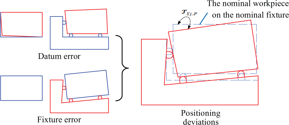
Positioning deviation.²⁵

The positioning deviation of a workpiece in setup j is the summation of datum errors, fixture errors, and link errors in the contact between the workpiece and the fixture. This is expressed in the SDT concept as shown in equation (1)

τ_{Sj, P} = - τ_{P, Pi} + τ_{Sj, Hk} + τ_{Hk, Pi}

(1)

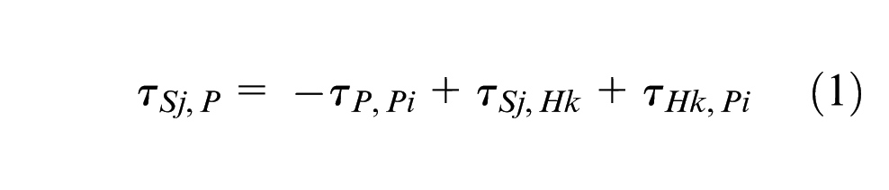
where $τ_{Sj, P}$ is the positioning deviation of setup j; $τ_{P, Pi}$ is the datum error, which is also known as the model of workpiece (MWP from the previous setup); τ_{Sj, Hk} is the fixture error of setup j; and $τ_{Hk, Pi}$ is the link error in the contact between the workpiece and the fixture in setup j.

Machining deviation

Many key factors can affect the accuracy of the machine tool. Thus, the machine tool can cause errors on the machined surface. The machining deviation is expressed as the deviation between the machined surface and the nominal surface created by the nominal machine tool (Figure 3).

Figure 3.

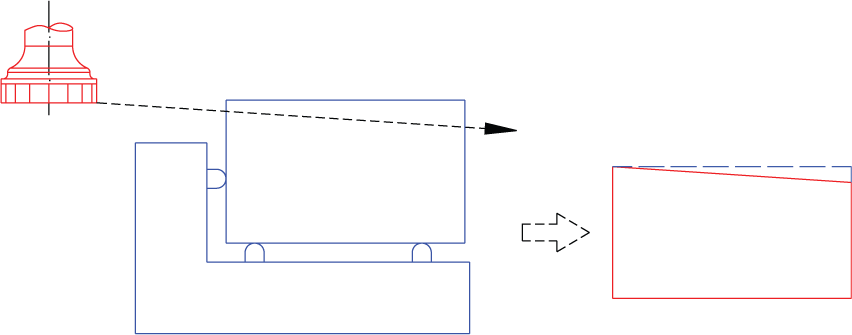
Machining deviation.²⁵

The deviations of a machined surface in a setup, for example, setup j, are expressed by an SDT, denoted by $τ_{Sj, Pi}$ . Hence, the deviations of a machined surface compared to its nominal surface are denoted by the SDT $τ_{P, Pi}$ . This can be expressed in relation to the positioning and machining deviations as shown in equation (2)

τ_{P, Pi} = - τ_{Sj, P} + τ_{Sj, Pi}

(2)

Positioning and machining defects

The above positioning and machining deviations are considered for one workpiece (machined part) during manufacturing. In this study, each machined surface has a deviation; a set of machined surface deviations will create a machined surface defect. Hence, each component of the SDT is considered as a part of a machined surface defect. The variability of an SDT component can be expressed by a PDF or by statistical parameters.

Creating a deviation domain from a functional tolerance type

Parts are most unlikely to be machined to exact dimensional or geometrical specifications. Tolerances are therefore used to define the allowable variability for certain geometrical dimensions or forms. They are also used to specify the shape, orientation, and location of features on a part. According to ISO 1101, geometrical tolerance specifies the zones within which a machined surface must fit, that is, tolerance zones.

There are different approaches to compare a machined part to its functional tolerances, such as the virtual gauge approach²⁶ or GapGP approach²⁷ (GapGP is the signed distance measured between the virtual gauge modeling the tolerance and the concerned surfaces of the MMP. The name of the variable GapGP has been chosen to abbreviate the Gap between the Gauge and the Part). In this study, deviation domains and tolerance zones are used for the comparison. To satisfy specifications, machined surface defects must be inside tolerance zones. As previously mentioned, considering that each machined surface has a deviation, a set of machined surface deviations will create a deviation domain. This depends on the types of machined part defects, for example, parallelism, perpendicularity, location, and so on. The following example illustrates the deviation domain of a parallelism defect.

A cylindrical part has two planes P1 and P2. Let P1 and P2 be two parallel planes that are expressed by two SDTs, let Z_CL be the cylinder axis, and let D be the nominal diameter of this part (Figure 4).

Figure 4.

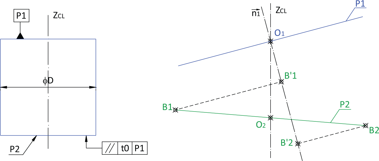
Parallelism defect.

If P1 is a reference plane, the parallelism defect of P2 is defined as distance $B'_{1} B'_{2}$ (Figure 4), where $B'_{1}$ and $B'_{2}$ are projected points of B₁ and B₂ on the normal vector $\vec{n_{1}}$ of P1. It is easy to see that this defect does not depend on the positions of these two planes. Equation (3) expresses the deviation domain of the parallelism defect of P2 compared to reference P1

\frac{\vec{B_{1} B_{2}} \vec{n_{1}}}{‖ \vec{n_{1}} ‖}

(3)

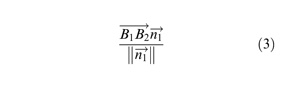
where B₁ and B₂ are the highest and lowest points on the border of the machined surfaces.

This formulation can be rewritten to include the parameters of the geometrical surface and the SDT components (see section “Tolerance analysis method: a case study”). Similarly, mathematical formulations of different types of functional tolerance can be created. These are then used for comparison with the values of the tolerance zones in order to validate a process plan or to obtain achievable functional tolerances taking into account a given ppm value.

Experimental manufacturing defects

The purpose of this section is to describe the method implemented to obtain the experimental manufacturing defects presented in the previous studies.^28–30 In this study, the manufacturing defects are divided into two main categories: machining defects and positioning defects. The method for identifying both types of defects is presented below. An experiment is described to clearly illustrate this method.

The experiment is based on a batch of 50 workpieces made of aluminum (2017 A) with a diameter of 30 mm and a length of 50 mm (Figure 5). A sawing machine is used to cut the 50 workpieces from a long aluminum bar. Two sawed surfaces and the cylindrical surface of a workpiece are considered as the initial state of production.

Figure 5.

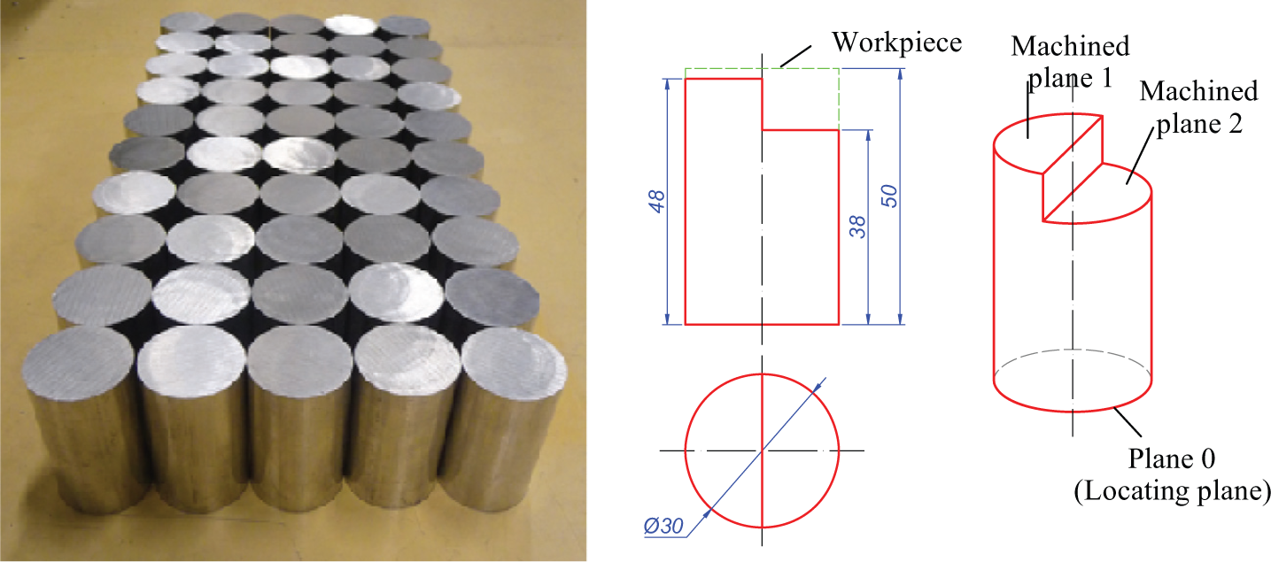
Workpieces and designed part.

A workpiece is first located and fixed on the computer numerical control (CNC) milling machine by a three-soft-jaw chuck (fixture). Two planes are machined by an end mill (φ20) with two different tool paths. The machined planes are measured with the touch probe just after the final cutting steps. The workpiece cylinders are also measured to identify one of the components of the positioning defects. The machined parts are then measured individually on the Coordinate Measuring Machine (CMM). This makes it possible to identify the rest of the components of the positioning defects (Figure 6).

Figure 6.

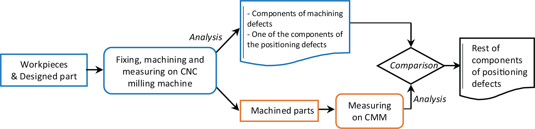
Identification of experimental data.

The MMP is used to express the machining deviations of the machined surfaces or the positioning deviations of the workpiece on the fixture in each setup. Errors in each setup accumulate on the workpiece and affect the machining accuracy in the subsequent setup. In the MMP, SDTs are used to express machined surface defects, that is, machining defects and positioning defects.

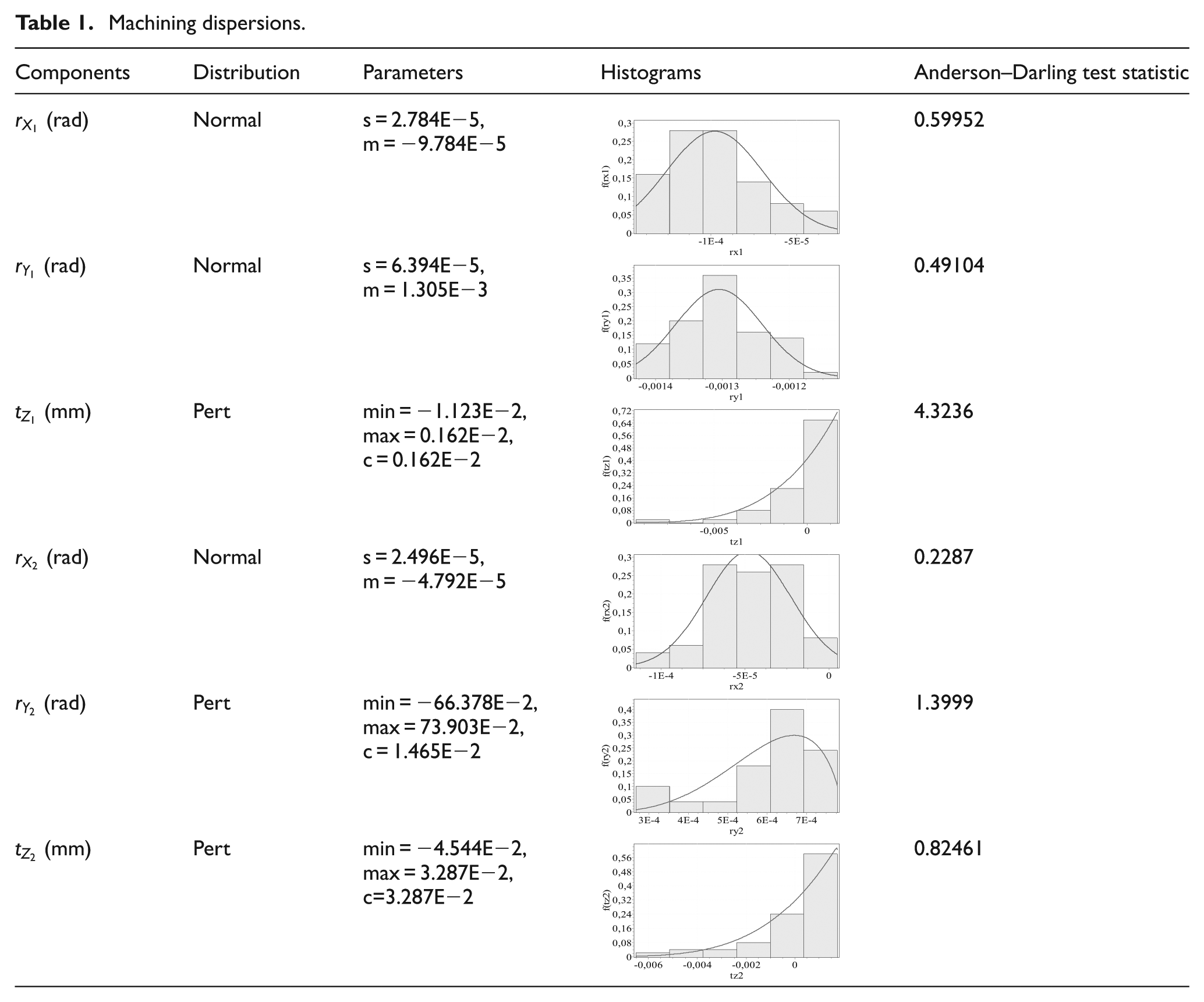
Each component of the machining and positioning defects is expressed as a probability distribution and a statistical parameter that can be used for simulations (e.g. Monte Carlo simulations). Statistical software (Easy-Fit) is used to determine the probability distributions and statistical parameters from the data set of each component (Tables 1 and 2). The values of Anderson–Darling test statistic are also provided. These values are calculated using the approximation formula and depend on the sample size only. This kind of test (compared to the “original” Anderson–Darling test) is less likely to reject the good fit and can be successfully used to compare the goodness of fit of several fitted distributions.

Table 1.

Machining dispersions.

Components	Distribution	Parameters	Anderson–Darling test statistic
$r_{X_{1}}$ (rad)	Normal	s = 2.784E−5, m = −9.784E−5	0.59952
$r_{Y_{1}}$ (rad)	Normal	s = 6.394E−5, m = 1.305E−3	0.49104
$t_{Z_{1}}$ (mm)	Pert	min = −1.123E−2, max = 0.162E−2, c = 0.162E−2	4.3236
$r_{X_{2}}$ (rad)	Normal	s = 2.496E−5, m = −4.792E−5	0.2287
$r_{Y_{2}}$ (rad)	Pert	min = −66.378E−2, max = 73.903E−2, c = 1.465E−2	1.3999
$t_{Z_{2}}$ (mm)	Pert	min = −4.544E−2, max = 3.287E−2, c=3.287E−2	0.82461

Table 2.

Positioning dispersions.

Components	Distribution	Parameters	Histograms	Anderson–Darling test statistic
$r_{X}$ (rad)	Normal	s = 5.604E−4, m = −6.712E−4		0.2085
$r_{Y}$ (rad)	Pert	min = −0.115E−2, max = −0.143E−2, c = −6.056E−4		0.55991

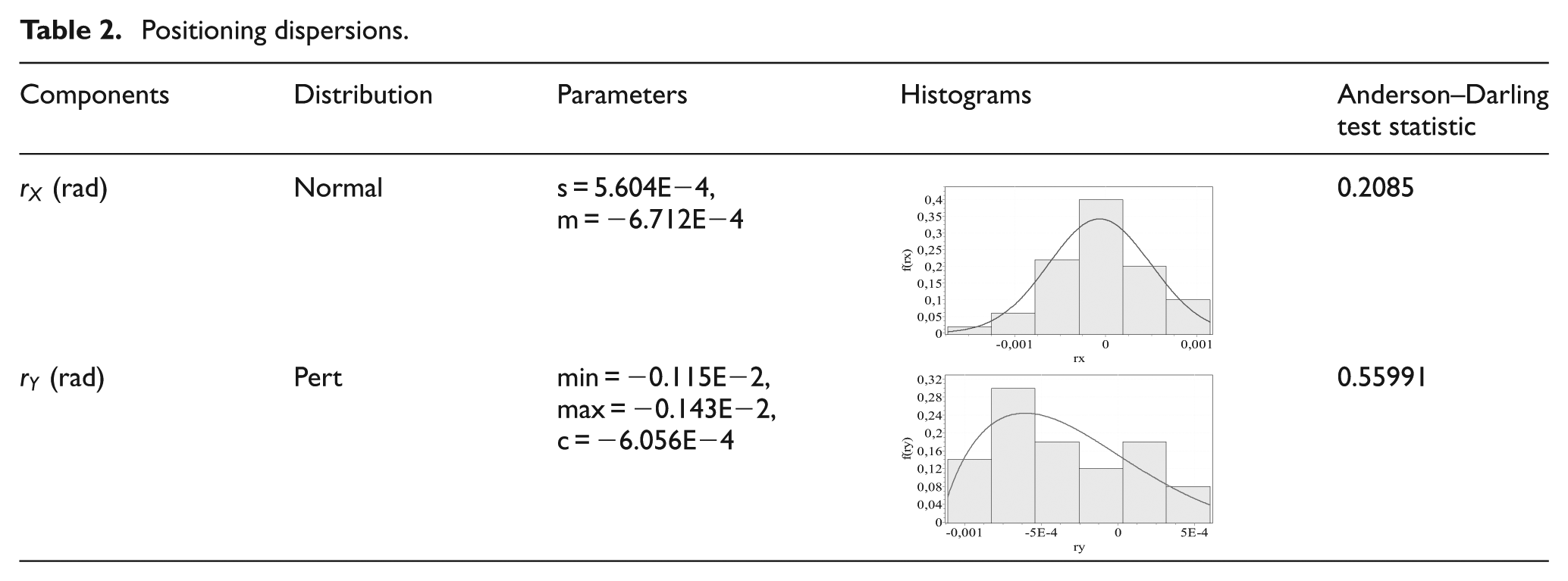
The results show that the manufacturing defects are not always normal distributions or uniform distributions as demonstrated in the propositions of other articles addressing the variables used in simulations. The PDFs of the experimental data can be used as input variables to analyze other process plans.

Tolerance analysis method: a case study

Description of the machined part and the process plan

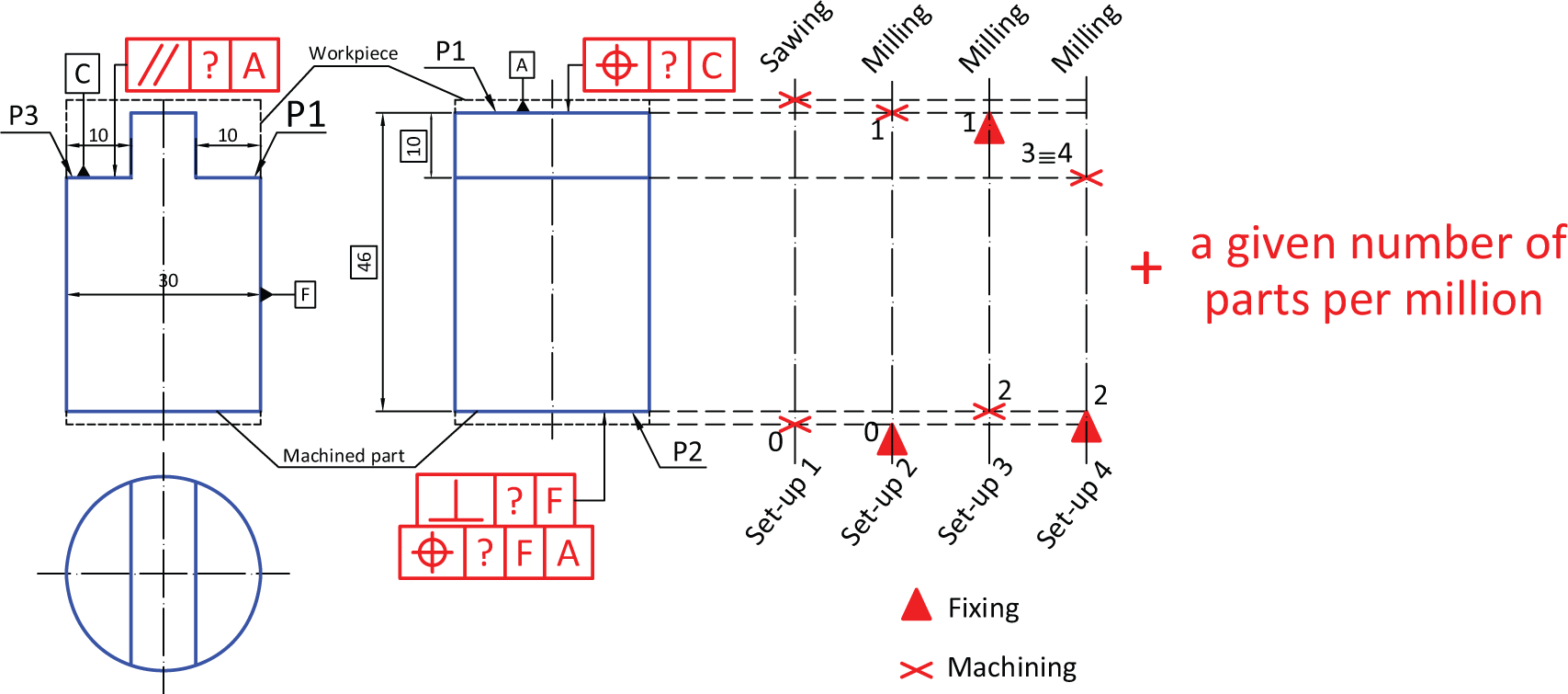
In this section, a machined part is used as an example for manufacturing tolerance analysis (Figure 7). There are two possible aims: to verify the process plan of a batch of machined parts or to determine compatible functional tolerances based on a given process plan and ppm. For example, a batch of machined parts that go through four setups with two types of machine tools (sawing machine and milling machine) can be investigated (Figure 8(a)). It is important to note that several parameters of this illustrative example are similar to the experimental application in the study of Bui et al.²⁸ (e.g. type of milling tool, tool paths, and dimensions of workpieces). The machined part and its process plan are illustrated as follows.

Figure 7.

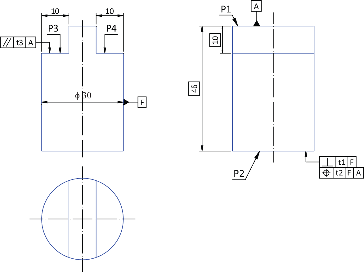
Machined part and functional tolerances.

Figure 8.

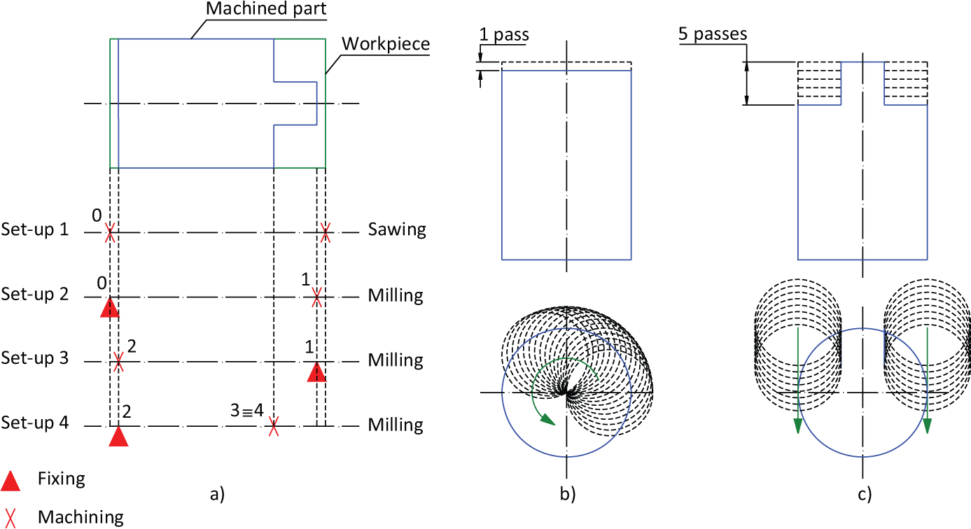
Process plan and tool paths.

The workpieces in this example are made of aluminum (2017 A) and have a diameter of 30 mm and a length of 50 mm. A sawing machine is used to cut the workpieces from a long aluminum bar. The workpieces are then located and fixed on a CNC milling machine by a three-soft-jaw chuck (fixture) in order to machine different planes.

Setup 1

A sawing machine is used to cut a length of 50 mm (L₀) of each workpiece. One of the cutting planes in this setup and the workpiece cylinder will be used to locate and fix the workpiece on a fixture in the next setup. Another cutting plane is the workpiece locating plane (P0).

Setup 2

The workpieces are then located and fixed on the fixture in a CNC milling machine so that their top surface, that is, P1, can be machined. A circular path is used to machine this plane with only one end mill pass (Figure 8(b)). The cutting depth of this pass is 2 mm. The machined part has a length of 48 mm (L₁) after this setup.

Setup 3

The workpiece in this setup is located and fixed according to P1, machined in setup 2, and the workpiece cylinder. A plane is machined following a circular path with only one pass of the milling tool and a cutting depth of 2 mm. The machined plane is called P2. The machined part has a length of 46 mm (L₂) after this setup.

Setup 4

The workpiece in this setup is located and fixed according to P2 and the workpiece cylinder. P3 and P4 are then machined by a straight-line path involving five passes of the end mill. The cutting depth of each pass is 2 mm. The final passes on P3 and P4 are shown in Figure 8(c). The distance from P3/P4 to P1 is 10 mm (L₄).

MMP

The MMP is used to express the machining deviations of the machined surfaces or the positioning deviations of the workpiece on the fixture in each setup. The errors in each setup are accumulated on the workpiece and affect the machining accuracy of the next setup. The SDT is used to express the machined surface defects, which may include machining defects and positioning defects. These defects are then used to determine the deviation domains.

SDT of the workpiece’s locating plane (P0)

Setup 1 (Figure 9(a))

Figure 9.

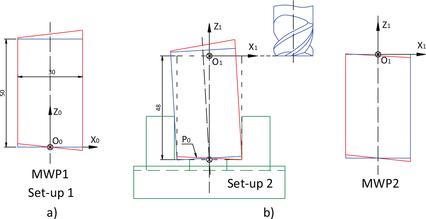
Setups 1 and 2.

The machining deviations are expressed by an SDT. It can be seen that only two rotations of the surface P0 will influence the machined surfaces in setup 2. The small translation of P0 is therefore negligible. Thus, we can express the SDT of P0 as follows

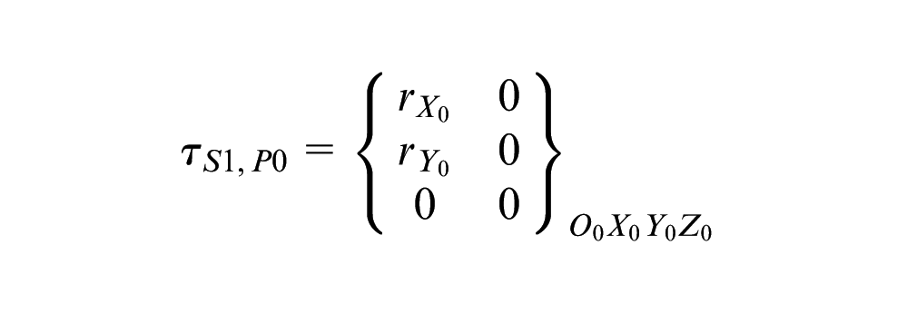
τ_{S 1, P 0} = {\begin{matrix} r_{X_{0}} & 0 \\ r_{Y_{0}} & 0 \\ 0 & 0 \end{matrix}}_{O_{0} X_{0} Y_{0} Z_{0}}

where $τ_{S 1, P 0}$ is the SDT of the machined plane P0 in setup 1 and $O_{0} X_{0} Y_{0} Z_{0}$ is the coordinate system of the nominal plane.

SDT of the machined plane P1

Setup 2 (Figure 9(b))

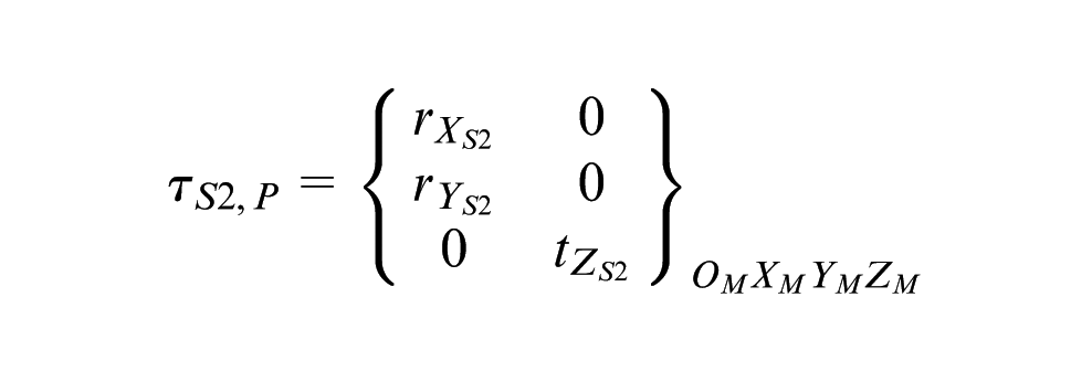
Vertical machined surface defects are not considered in this study. Hence, translations along the X- and Y-axes of the workpiece on the fixture are not needed in this case. The positioning deviation of the workpiece on the fixture in setup 2 is expressed by an SDT that includes two rotations of the workpiece cylinder around the X- and Y-axes $(r_{X_{S 2}}, r_{Y_{S 2}})$ and the translation along the Z-axis $(t_{Z_{S 2}})$

τ_{S 2, P} = {\begin{matrix} r_{X_{S 2}} & 0 \\ r_{Y_{S 2}} & 0 \\ 0 & t_{Z_{S 2}} \end{matrix}}_{O_{M} X_{M} Y_{M} Z_{M}}

where $O_{M} X_{M} Y_{M} Z_{M}$ is the machine coordinate system (MCS).

Machined plane P1

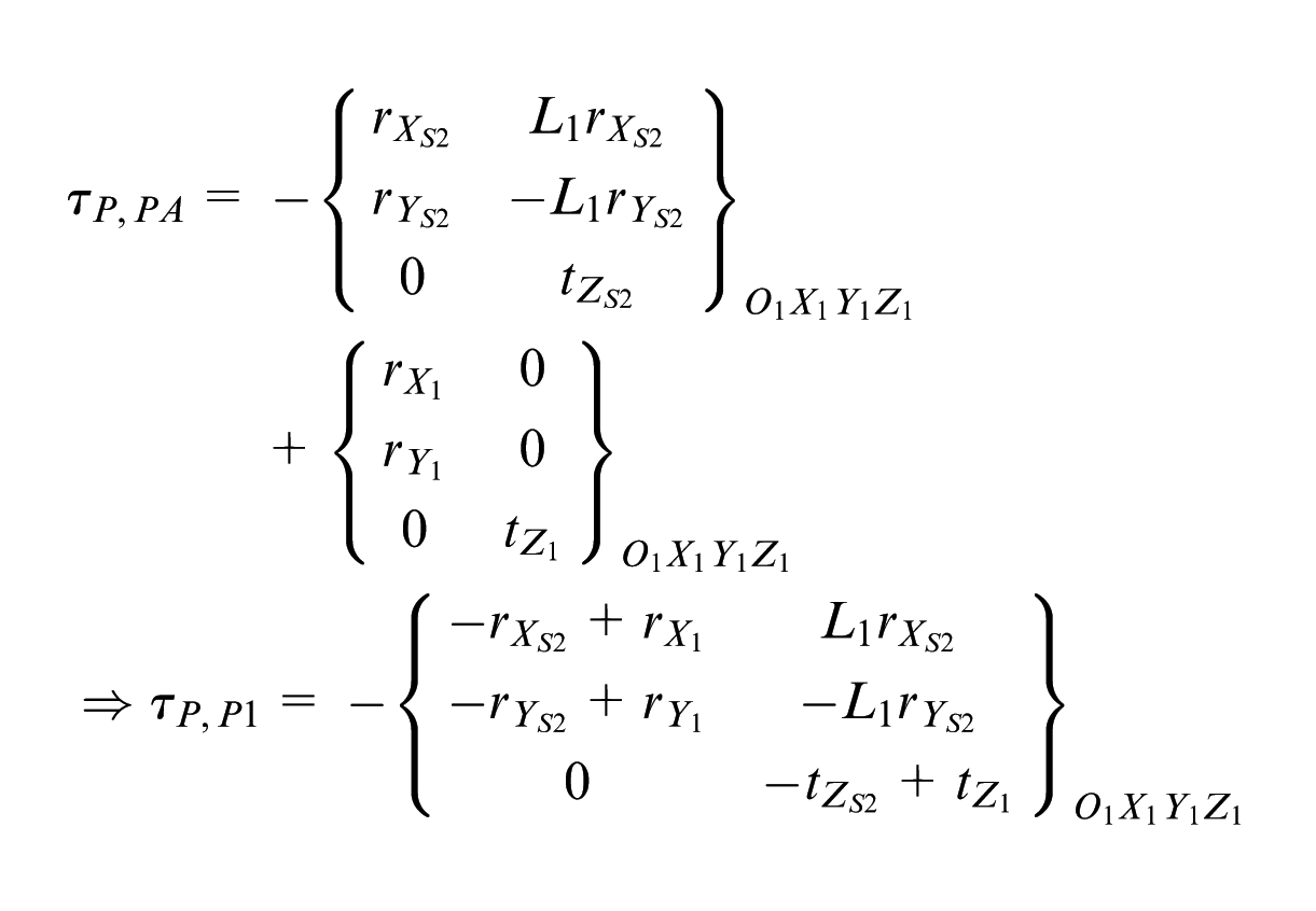
The machining deviation of machined plane P1 compared to its nominal plane is expressed in the following equation

τ_{P, P 1} = - τ_{S 2, P} + τ_{S 2, P 1}

τ_{P, P 1} = - {\begin{matrix} r_{X_{S 2}} & 0 \\ r_{Y_{S 2}} & 0 \\ 0 & t_{Z_{S 2}} \end{matrix}}_{O_{M} X_{M} Y_{M} Z_{M}} + {\begin{matrix} r_{X_{1}} & 0 \\ r_{Y_{1}} & 0 \\ 0 & t_{Z_{1}} \end{matrix}}_{O_{1} X_{1} Y_{1} Z_{1}}

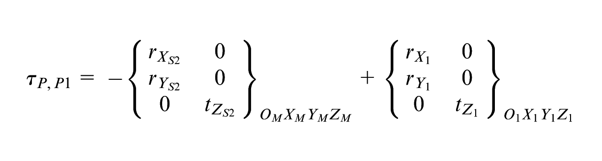
where $τ_{S 2, P 1}$ is the SDT of the machining deviation of machined plane P1 in setup 2 and $τ_{S 2, P}$ is the SDT of the positioning deviation of the workpiece on the fixture in setup 2.

The torsor $τ_{S 2, P}$ can be rewritten into the $O_{1} X_{1} Y_{1} Z_{1}$ system by changing the frame as follows

τ_{S 2, P} = {\begin{matrix} \vec{R} {\vec{T}}_{OM} \end{matrix}}_{O_{M} X_{M} Y_{M} Z_{M}} = {\begin{matrix} \vec{R} {\vec{T}}_{OM} + \vec{R} \land \vec{O_{M} O_{1}} \end{matrix}}_{O_{1} X_{1} Y_{1} Z_{1}}

where

τ_{S 2, P} = {\begin{matrix} 0 \\ 0 \\ t_{Z_{S 2}} \end{matrix}} + {\begin{matrix} r_{X_{S 2}} \\ r_{Y_{S 2}} \\ 0 \end{matrix}} \land {\begin{matrix} 0 \\ 0 \\ L_{1} \end{matrix}} = {\begin{matrix} L_{1} r_{X_{S 2}} \\ - L_{1} r_{Y_{S 2}} \\ t_{Z_{S 2}} \end{matrix}}

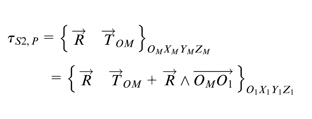
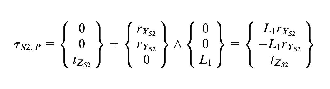
where L₁ is the length of the machined part after setup 2.

Therefore,

\begin{matrix} τ_{P, PA} = - {\begin{matrix} r_{X_{S 2}} & L_{1} r_{X_{S 2}} \\ r_{Y_{S 2}} & - L_{1} r_{Y_{S 2}} \\ 0 & t_{Z_{S 2}} \end{matrix}}_{O_{1} X_{1} Y_{1} Z_{1}} \\ + {\begin{matrix} r_{X_{1}} & 0 \\ r_{Y_{1}} & 0 \\ 0 & t_{Z_{1}} \end{matrix}}_{O_{1} X_{1} Y_{1} Z_{1}} \\ \Rightarrow τ_{P, P 1} = - {\begin{matrix} - r_{X_{S 2}} + r_{X_{1}} & L_{1} r_{X_{S 2}} \\ - r_{Y_{S 2}} + r_{Y_{1}} & - L_{1} r_{Y_{S 2}} \\ 0 & - t_{Z_{S 2}} + t_{Z_{1}} \end{matrix}}_{O_{1} X_{1} Y_{1} Z_{1}} \end{matrix}

The SDTs of machined planes 2 and 3 can also be obtained. Hence, the SDTs of the machined planes are summarized in Table 3.

Table 3.

The SDTs of the machined planes.

Machined plane	SDT
P1	$τ_{P, P 1} = - {\begin{matrix} - r_{X_{S 2}} + r_{X_{1}} & L_{1} r_{X_{S 2}} \\ - r_{Y_{S 2}} + r_{Y_{1}} & - L_{1} r_{Y_{S 2}} \\ 0 & - t_{Z_{S 2}} + t_{Z_{1}} \end{matrix}}_{O_{1} X_{1} Y_{1} Z_{1}}$
P2	$τ_{P, P 2} = - {\begin{matrix} - r_{X_{S 3}} - r_{X_{2}} & L_{2} r_{X_{S 3}} - L_{2} r_{Y_{S 3}} + L_{2} r_{Y_{2}} \\ - r_{Y_{S 3}} + r_{Y_{2}} & L_{2} r_{Y_{S 3}} - L_{2} r_{X_{S 3}} + L_{2} r_{X_{2}} \\ 0 & t_{Z_{S 3}} - t_{Z_{2}} \end{matrix}}_{O_{1} X_{1} Y_{1} Z_{1}}$
P3	$τ_{P, P 3} = - {\begin{matrix} - r_{X_{S 4}} + r_{X_{3}} & - L_{2} r_{Y_{S 4}} + L_{4} r_{Y_{3}} \\ - r_{Y_{S 4}} + r_{Y_{3}} & L_{2} r_{X_{S 4}} - L_{4} r_{X_{3}} \\ 0 & - t_{Z_{S 4}} - \frac{4 R \sin^{3} (θ / 2)}{3 (θ - \sin θ)} r_{Y_{3}} + t_{Z_{3}} \end{matrix}}_{O_{1} X_{1} Y_{1} Z_{1}}$

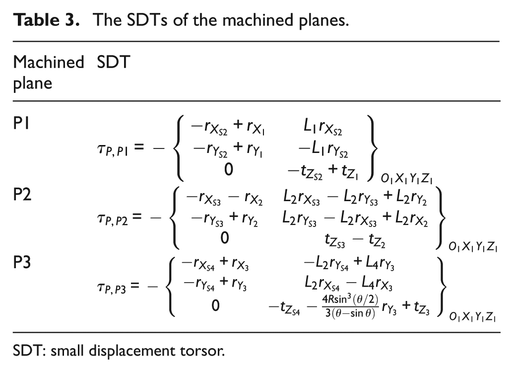
SDT: small displacement torsor.

Relationship between the MMP and the deviation domain

As mentioned previously, the MMP is based on the SDT that does not take into account machined surface form defects. Thus, only orientation and positional tolerance are considered in the following mathematical formulations. The formulations are applied for each machined surface of a batch of machined parts. The following example is used to determine the mathematical formulation of the perpendicularity defect of plane P2 compared to cylinder axis F.

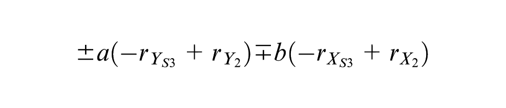
For perpendicularity tolerance, which reflects orientation, only rotational components are needed. Indeed, in this case, the position of the plane, compared to its nominal coordinate system, is not important. Thus, to analyze the ability of the process plan to achieve the right perpendicularity, component $\vec{δ P} . \vec{Z} - t_{Z}$ must be limited to within the tolerance zone (0, t). Two contacting points delimiting tolerance zones B₁ and B₂ (Figure 10) are defined by the equation below

\pm a (- r_{Y_{S 3}} + r_{Y_{2}}) \mp b (- r_{X_{S 3}} + r_{X_{2}})

Figure 10.

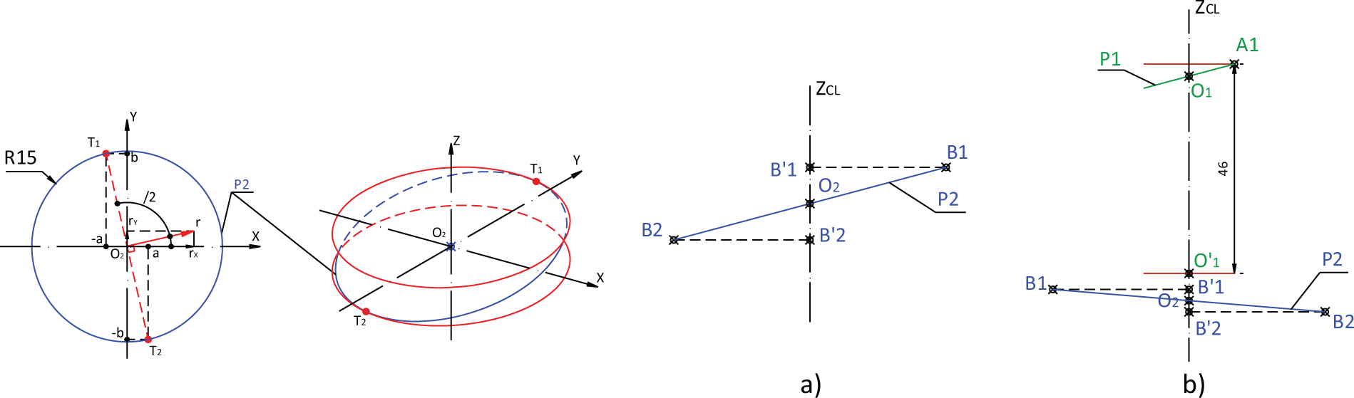
Perpendicularity and location defect of P2.

The mathematical formulation, which will be used to verify the perpendicularity tolerance of machined plane P2, is expressed in formula (4)

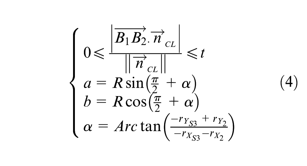
{\begin{matrix} 0 \leq \frac{| \vec{B_{1} B_{2}} . {\vec{n}}_{CL} |}{‖ {\vec{n}}_{CL} ‖} \leq t \\ a = R \sin (\frac{π}{2} + α) \\ b = R \cos (\frac{π}{2} + α) \\ α = Arc \tan (\frac{- r_{Y_{S 3}} + r_{Y_{2}}}{- r_{X_{S 3}} - r_{X_{2}}}) \end{matrix}

(4)

The components $- r_{Y_{S 3}} + r_{Y_{2}}$ and −r_{X
_S3} − r_{X
₂} in formula (4) are considered as input variables in simulations of tolerance analysis. These input variables are generated by a Monte Carlo simulation based on the PDFs of the machined surfaces obtained from the experiments (see section “Experimental manufacturing defects”).

Similarly, the mathematical formulations of the location defect of plane P2 and the parallelism defect of plane P3 can be determined.

Process plan verification

One hundred thousand parts are virtually manufactured using the Monte Carlo simulation method and according to the process plan in Figure 8(a) and the functional tolerances in Figure 7. The defects of each machined surface are then compared to their functional tolerances (see formula (4) for the case of perpendicularity). Table 4 shows the results of the simulation in the form of histograms with the associated statistics (estimation of the mean value, variance, skewness, and kurtosis) as well as the number of rejected parts.

Table 4.

Simulation to verify the process plan.

Machined surface planes	Functional tolerance		Histograms	Rejected parts
P₂	Perpendicularity (versus F)	0.09	m = 26.603E−03, s = 0.312E−03, skewness = 0.633, kurtosis = 2.952	97/100,000
	Location (versus F and A)	0.4	m = 107.052E−03, s = 4.157E−03, skewness = 1.075, kurtosis = 4.663	99/100,000
P₃	Parallelism (versus A)	0.08	m = 31.598E−03, s = 0.207E−03, skewness = 0.436, kurtosis = 2.916	108/100,000

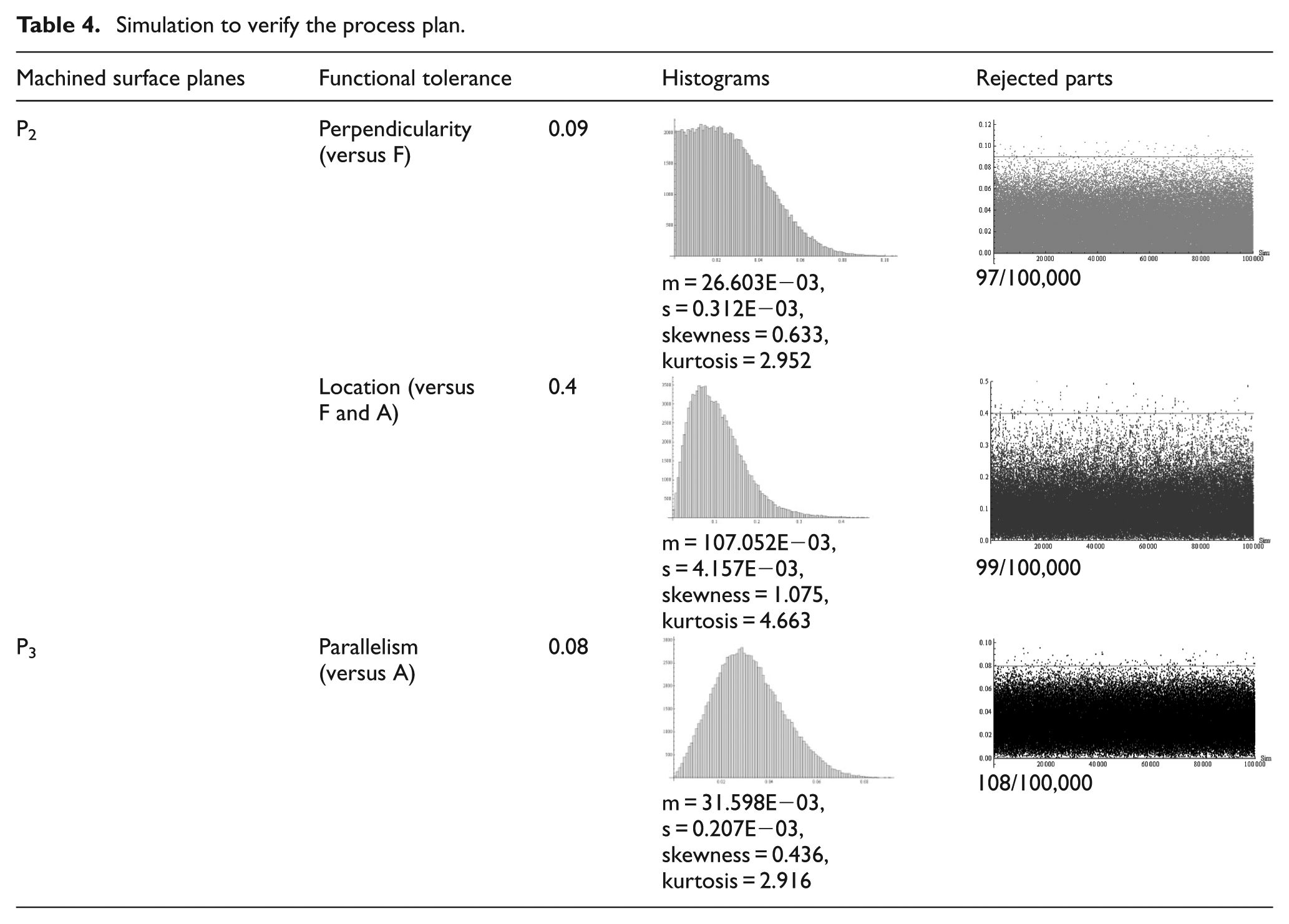
Table 4 shows the histograms of each simulated functional tolerance and the rejected parts per 100,000 iterations. It can be used to verify the proposed process plan. For instance, with the functional tolerance given in Table 4 and a number of rejected parts of up to 100 ppm (10 parts per 100,000), the above process plan is not satisfactory.

Thanks to the Monte Carlo simulation, the values of the achievable functional tolerances can be determined to ensure the validity of an existing process plan with a given number of ppm. These are outlined in what follows.

Determination of achievable functional tolerance values for a given number of ppm

The objective is to determine the achievable tolerances of a part based on a given process plan and ppm (Figure 11).

Figure 11.

A process plan and a given number of parts per million (ppm).

Table 5 shows the predicted tolerance values that ensure 100 ppm if the above process plan is used for manufacturing.

Table 5.

Predicted functional tolerances.

Machined surface planes	Predicted tolerances for 100 ppm (mm)		Initial tolerances (mm)
P₂	Perpendicularity (versus F)	0.1	0.09 (970 ppm)
	Location (versus F and A)	0.485	0.4 (990 ppm)
P₃	Parallelism (versus A)	0.09	0.08 (1080 ppm)

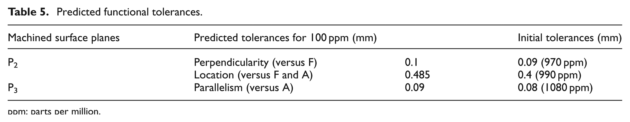
ppm: parts per million.

The initial tolerances given in Table 4 are also presented in Table 5 to clearly show the differences between the two simulations. For instance, if the initial tolerance of the location between machined plane P2 (B) and cylinder F and plane A is 0.4, the amount of rejected ppm is 990. Thus, in order to bring the number down to 100 ppm, the location tolerance must be expanded from 0.4 to 0.485.

Conclusion

This article proposes detailed mathematical formulations for use in manufacturing tolerance analysis in which the input variables are generated from the experimental data. The deviation domains of each machined surface are first created based on the types of functional tolerance. The given process plan is modeled using the MMP method. The mathematical formulations of the functional tolerances are then rewritten to include the parameters of the MMP and the deviation domains. The formulations are finally used in tolerance analysis for:

verification of a process plan in terms of the functional tolerances of a batch of machined parts or

determination of the achievable tolerances of machined parts based on an existing process plan and requirement in terms of rejected ppm.

The simulation is performed based on the results of a particular case where the aim is to obtain the experimental PDFs of manufacturing defects. The model based on MMP can be applied to different cases, but the Monte Carlo simulation of this model needs to use the experimental PDF. It is easy to see that if the distributions of the input variables match the real results, the output is closer to the real production. A summary of the method used to obtain experimental manufacturing defects is provided. As part of future research work, we propose to use the response surface methodology in simulations of manufacturing defects in which the experimental defects obtained will be considered.

To obtain the input variables for Monte Carlo simulations, several proposals can be put forward for future work:

analysis of the manufacturing defects of a sample batch of machined parts before machining a large batch of parts and

creation of libraries of manufacturing defects relating to different types of fixture and machined surface (a more costly and time-consuming project than the first).

Footnotes

Funding

This research was made possible by funding from Cluster gospi (Rhone-Alpes region), SYMME laboratory - University of Savoie, and G-SCOP laboratory - University of Grenoble, France.

References

Singh

Jain

. Important issues in tolerance design of mechanical assemblies. Part 1: tolerance analysis. Proc IMechE, Part B: J Engineering Manufacture 2009; 223: 1225–1247.

Marziale

Polini

. Review of variational models for tolerance analysis of an assembly. Proc IMechE, Part B: J Engineering Manufacture 2011; 225: 305–318.

Bourdet

. Chaines de cotes de fabrication (Methode des delta l): premiere partie “Modeles”: L’lngenieur et le Technicien de l’Enseignement Technique; Decembre 1973. (http://www.lurpa.ens-cachan.fr/~bourdet/Publi_theme.htm)

Asante

. A small displacement torsor model for tolerance analysis in a workpiece-fixture assembly. Proc IMechE, Part B: J Engineering Manufacture 2009; 223: 1005–1020.

Rivest

Fortin

Morel

. Tolerancing a solid model with a kinematic formulation. Comput Aided Design 1994; 26: 465–476.

Laperrière

Lafond

. Tolerance analysis and synthesis using virtual joints. In: Proceedings of the 6th CIRP international seminar on computer-aided tolerancing, Enschede, The Netherlands, 1999. Published: Dordrecht; Boston: Kluwer Academic, c1999.(http://trove.nla.gov.au/work/28876234?q=%22+Tolerance+%28Engineering%29+Data+processing+Congresses.%22&c=book&versionId=45848391)

Laperrière

ElMaraghy

. Tolerance analysis and synthesis using Jacobian transforms. CIRP Ann: Manuf Techn 2000; 49: 359–362.

Desrochers

Rivière

. A matrix approach to the representation of tolerance zones and clearances. Int J Adv Manuf Tech 1997; 13: 630–636.

Whitney

Gilbert

. Representation of geometric variations using matrix transforms for statistical tolerance analysis in assemblies. In: IEEE international conference on robotics and automation, Atlanta, GA, 2–6 May 1993. Page(s): 314 - 321 vol.2; Product Type: Con ference Publications; Print ISBN: 0-8186-3450-2; INS PEC Accession Number: 4687303; Digital Object Identifier:10.1109/ROBOT.1993.292164; Date of Current Version: 06 août 2002; Issue Date: 2–6 May 1993 (http://ieeexplore.ieee.org/xpl/login.jsp?tp=&arnumber=292164&url=http%3A%2F%2Fieeexplore.ieee.org%2Fxpls%2Fabs_all.jsp%3Farnumber%3D292164)

10.

Wirtz

. Vectorial tolerancing a tool for functional analysis. In: Proceeding of the 3rd CIRP seminar on Computer Aided Tolerancing, France, 1993. Editions Eyrolles ISBN:2-212-08779-9, pp. 115–128.

11.

Wirtz

Gaechter

Wipf

. From unambiguously defined geometry to the perfect quality control loop. CIRP Ann: Manuf Techn 1993; 42: 615–618.

12.

Martinsen

. Vectorial tolerancing for all types of surfaces. Advanced in Design Automation - ASME. 1993; vol 2: 187–98.

13.

Bourdet

Mathieu

Lartigue

Ballu

. The concept of the small displacement torsor in metrology. Advanced Mathematical Tools in Metrology II, Series Advances in Mathematics for Applied Sciences: World Scientific. River Edge, NJ: World Scientific Publishing, 1996, pp 110–122.

14.

Giordano

Kataya

Pariel

. Tolerance analysis and synthesis by means of clearance and deviation spaces. In: Geometric product specification and verification: Integration of functionality. Kluwer Academic Publishers, 2003, pp. 145–154. Selected Conference Papers of the 7th CIRP International Seminar on Computer-Aided Tolerancing, held at the Ecole Normale Supérieure de Cachan, France, 24-25 April 2001. Edited by BOURDET Pierre; MATHIEU Luc.(http://www.springer.com/engineering/computational+intelligence+and+complexity/book/978-1-4020-1423-9)

15.

Teissandier

Couétard

Gérard

. A computer aided tolerancing model: proportioned assembly clearance volume. Comput Aided Design 1999; 31: 805–817.

16.

Huang

Shi

Yuan

. Part dimensional error and its propagation modeling in multi-operational machining processes. J Manuf Sci E: T ASME 2003; 125: 255–262.

17.

Ding

Ceglarek

Shi

. Fault diagnosis of multistage manufacturing processes by using state space approach. J Manuf Sci E-T ASME 2002; 124: 313–322.

18.

Zhou

Huang

Shi

. State space modeling of dimensional variation propagation in multistage machining process using differential motion vectors. IEEE T Robotic Autom 2003; 19: 296–309.

19.

Loose

Zhou

Ceglarek

. Kinematic analysis of dimensional variation propagation for multistage machining processes with general fixture layouts. IEEE T Autom Sci Eng 2007; 4(2): 141–152.

20.

Villeneuve

Legoff

Landon

. Tolerancing for manufacturing: a three-dimensional model. Int J Prod Res 2001; 39: 1625–1648.

21.

Vignat

Villeneuve

. 3D transfer of tolerances using a SDT approach: application to turning process. J Comput Inf Sci Eng 2003; 3: 45–53.

22.

Villeneuve

Vignat

. Manufacturing Process Simulation for Tolerance Analysis and Synthesis. In: Bramley

Brissaud

Coutellier

McMahon

editors. Advances in Integrated Design and Manufacturing in Mechanical Engineering: Springer Netherlands; 2005. pp. 189–200.

23.

Vignat

Villeneuve

Kamali Nejad

. From the nominal model to a model of manufactured parts in a CAD context. Asian Int J Sci Tech Prod Manuf Eng 2009; 2: 35–42.

24.

Villeneuve

Vignat

. Manufacturing Process Simulation for Tolerance Analysis and Synthesis. In: Bramley

Brissaud

Coutellier

McMahon

editors. Advances in Integrated Design and Manufacturing in Mechanical Engineering: Springer Netherlands; 2005. pp. 189–200.

25.

Kamali Nejad

. Proposition de résolution numérique des problème d’analyse de tolérance en fabrication: approache 3D. PhD Thesis, University of Joseph Fourier, France, 2009.

26.

Mailhe

Linares

Sprauel

. Geometrical checking by virtual gauge, including measurement uncertainties. CIRP Ann: Manuf Techn 2008; 57: 513–516.

27.

Kamali Nejad

Vignat

Villeneuve

. Simulation of the geometrical defects of manufacturing. Int J Adv Manuf Tech 2009; 45: 631–648.

28.

Bui

Villeneuve

Sergent

. Evaluation of different methods in quantification of manufacturing defects. Asian Int J Sci Tech Prod Manuf Eng 2011; 4: 1–12.

29.

Bui

Sergent

Villeneuve

. Assessment of the impact of calculation methodologies on defect determinations in manufacturing. In: The international conference on integrated design and manufacturing in mechanical engineering, Bordeaux, France, 20–22 October 2010, IDMME P106. Springer Verlag Publishing.

30.

Sergent

Bui

Favreliere

. Identification of machining defects by small displacement torsor and form parameterization method. In: The international conference on Integrated design and manufacturing in mechanical engineering, Bordeaux, France, 20–22 October 2010, IDMME P27. Springer Verlag Publishing.

Manufacturing tolerance analysis based on the model of manufactured part and experimental data

Abstract

Keywords

Introduction and literature review

Overview of the MMP

Positioning deviation

Machining deviation

Positioning and machining defects

Creating a deviation domain from a functional tolerance type

Experimental manufacturing defects

Tolerance analysis method: a case study

Description of the machined part and the process plan

MMP

SDT of the workpiece’s locating plane (P0)

SDT of the machined plane P1

Relationship between the MMP and the deviation domain

Process plan verification

Determination of achievable functional tolerance values for a given number of ppm

Conclusion

Footnotes

Funding

References