Sage Journals: Discover world-class research

Abstract

Nowadays, the management of product geometrical variations during the whole product development process is an important issue for companies’ competitiveness. During the design phase, geometric functional requirements and tolerances are derived from the design intent. Furthermore, the manufacturing and measurement stages are two main geometric variations generators according to the two well-known axioms of manufacturing imprecision and measurement uncertainty. GeoSpelling as the basis of the geometrical product specification standard enables a comprehensive modeling framework and an unambiguous language to describe geometric variations covering the overall product lifecycle thanks to a set of concepts and operations based on the fundamental concept of the “Skin Model.” In contrast, only few research studies have focused on the skin model representation and simulation. The skin model as a discrete shape model is the main focus of this work. We investigate here discrete shape and variability modeling fundamentals, Markov Chain Monte Carlo simulation techniques and statistical shape analysis methods to represent, simulate, and analyze skin models. By means of a case study based on a cross-shaped sheet metal part, the results of the skin model simulations are shown here, and the performances of the simulations are described.

Keywords

Geometrical product specification discrete shape modeling skin model Monte Carlo simulation discrete differential geometry

Introduction

In modern production engineering, new complex products with controlled tolerances are being increasingly adopted to improve companies’ market position. Geometric variations are inevitably generated during the manufacturing stage due to the accuracy of manufacturing technologies.¹ Geometric variations are also generated during the measurement stage considering measurement uncertainty.²

Within the context of product lifecycle management (PLM), information communication and sharing requires to manage the geometric variations along the whole product lifecycle. The geometric variations should be considered early in the tolerancing process in the design stage.³ Many computer-aided tolerancing (CAT) tools can help designers for functional tolerance specification, but they are limited to control the geometric variations when covering the whole product lifecycle. Different modeling frameworks have been proposed to build coherent and complete tolerancing process along the whole product lifecycle.

Hillyard and Braid⁴ developed the concept of variational geometry that is a dimension-driven, constraint-based technique. Another early example of previous work of tolerance-modeling technique is the solids offset approach proposed by Requicha,⁵ in which the tolerance zones of workpieces are obtained by “offsetting” the nominal boundaries. Bourdet⁶ developed the concept of the small displacement torsor (SDT) to solve the general problem of the fit of a geometric surface model to a set of points using rigid body movements. Based on the solids offset approach, Jayaraman and Srinivasan proposed virtual boundary requirement (VBRs) and conditional tolerance (CTs) approach.^7,8 Etesami⁹ formalizes the solids offset model and proposed using tolerance specification language (TSL) to describe tolerance constraints. Shah et al.¹⁰ proposed a dimension and geometric model, which is based on the relative degrees of freedom of geometric entities: feature axes, edges, faces, and features-of-size. Roy et al.¹¹ presented a mathematical scheme for interpreting dimensional and geometric tolerances for polyhedral parts in a solid modeler.

Among them, GeoSpelling proposed by Ballu and Mathieu,¹² as the basis of the geometrical product specification (GPS) standard, enables a comprehensive modeling framework and an unambiguous language to describe geometric variations covering the overall product lifecycle thanks to a set of concepts and operations based on the fundamental concept of the “Skin Model.” Different from the nominal model that is deemed as an ideal representation, the skin model is a shape model to represent non-perfect shapes.¹³ To the best knowledge of the authors of this article, the operationalization of GeoSpelling has not been successfully completed and few research studies have focused on the skin model representation and simulation.

In ISO 17450-1,¹³ a skin model is a shape model. Early researches in tolerance-based modeling lead to the development of attribute-based systems.¹⁴ These efforts could be roughly classified either as point-based (e.g. point cloud), surface/shell-based, or volume-based.¹⁵ A shape representation scheme can be defined as a mapping from a computer structure to a well-defined mathematical model that defines the notion of the physical object in terms of computable mathematical properties and is independent of any particular representation scheme.¹⁶ Johnson¹⁷ proposed a tolerance representation approach, which integrates dimensioning and tolerancing modelers with the geometric modelers. This B Rep–based model is applicable only for location and size tolerances, and it is limited to geometric entities such as planar faces, cylindrical faces, conical faces, and spherical faces. Requicha¹⁸ proposed a constructive solid geometry (CSG) -based tolerancing representation model, which is named as PADL-I and PADL-II modeler. The limitation of this CSG-based approach is that all of non-primitive faces derived from the same primitive face receive the same variations. Gossard et al.¹⁹ proposed a similar feature-based design system, which combines B-Rep solid model and GSG-representational scheme. This approach can be employed on a polyhedral solid model, but it is limited to the conventional tolerance representation.

Considering dense point data can be acquired by scanning techniques and discrete shapes are commonly used in production engineering, this research work focuses on discrete skin representation and simulation. It would also be efficient for the operationalization of GeoSpelling based on discrete skin model representation. Based on discrete skin model, discrete geometry processing techniques will enhance GeoSpelling-computing capabilities and enable its operationalization.²⁰

In order to enrich the skin model when considering the deviations from the nominal or computer-aided design (CAD) model, the authors have assessed the geometric deviations at many different scales. Kurfess and Banks²¹ modeled the manufacturing error using a sequence of models based on statistical hypothesis testing of the fitted residuals. Yang and Jackman²² evaluated form error using statistical method without independently analyzing the statistical properties of the associated residuals. Samper and Formosa²³ proposed a way to define form error parameters based on the eigenshapes of natural vibrations of surfaces. The originality of this method is that the set of form parameters can be computed for any kind of shape.

In this article, the authors investigate Markov Chain Monte Carlo (MCMC) simulation techniques and statistical shape analysis (SSA) methods to represent, simulate, and analyze skin models. A global-modeling approach based on principal component analysis (PCA) and a local modeling approach based on augmented Darboux frame is considered here. The local–global modeling approach enables the simulation of both random and systematic deviations when considering geometric constraint requirements, tolerance specifications, and manufacturing. In addition to discrete shape modeling for skin model representation and simulation, the concept of the mean skin model and its robust statistics are also introduced in this work.

The remainder of this article is organized as follows: first, the Monte Carlo simulation techniques and local/global modeling approaches for discrete skin model simulation will be introduced; second, the SSA for discrete skin models will be addressed; and finally, a case study to apply the proposed methods will be presented.

Skin model simulation

Skin model is a representation of real shapes. The geometric characteristics of real shapes should be fully considered for skin model shaping. In Caskey et al.,²⁴ the geometric deviations of the real surface to the nominal one are caused by two kinds of deviations: random deviations and systematic deviations. In this article, both are simulated to construct a complete skin model. Considering a designed shape is specified with geometric tolerances, the simulated skin models are located within the specified tolerance zones, which can be defined as constraints of skin model generation methods.²⁵ In this research, the deviations caused by random errors follow Gaussian (normal) distribution, which has been proven to be reasonable for mechanical applications,²⁶ while systematic deviations are reproducible inaccuracies that follow recognizable signatures, which can be calculated or simulated from target shapes.

Random deviation simulation based on MCMC

Random simulation techniques can be classified into physical and computational methods. The computational random simulation numbers are obtained by computational algorithms, which produce long sequences of apparently random results. Actually, the computational random numbers are pseudorandom, and they are determined by the initial value of the algorithm. Based on the hypothesis that the random deviations follow Gaussian distribution, three statistical methods have been developed for random deviation simulation: one-dimensional (1D) Gaussian, multi-Gaussian, and Gibbs methods.²⁵ The results of the Gaussian methods are influenced by the selection of the initial seed value. However, Gibbs methods are initial seed-independent. In this section, the Gibbs method is discussed in detail.

Gibbs method defined here is used to simulate the multi-Gaussian distribution of random numbers using the MCMC methods. The MCMC method generates a sequence of samples from the joint probability distribution of two or more random variables by iterative process. These methods are based on constructing a Markov chain that has the desired distribution and only depends on current state instead of the entire past data. Hence, Gibbs method provides reliable Gaussian distribution results.

In Gibbs sampling, a vector of parameters of interest $Ψ$ is required, and also a nuisance parameter $Λ$ with observed data $B$ , from which a converging distribution can be obtained. Suppose $(Ψ_{1} (0), Ψ_{2} (0), \dots, Ψ_{d} (0))$ is an initial starting random value in $R^{d}$ . Note that the conditional density function of $Ψ_{j} | Ψ_{- j}$ is $f (Ψ_{j} | Ψ_{- j})$ , from which the Gibbs sampler selects candidate points. The initialization of the process is at $t = 0$ and the initial vector value is then $Ψ (0)$ . When $t$ is increasing ( $t = 1, 2, \dots, T$ ), then $Ψ (t)$ follows the density function $f (Ψ_{j} | Ψ_{- j})$ and generates new point to replace the old one, and an iterative calculation is performed until it converges to the target value. The corresponding pseudo-code is described as follows

For $t = 1, 2, \dots, T$ , let $ψ_{1} = Ψ_{1} (t - 1)$ .

Let $j$ be a variable between [ $1, d$ ]. For $j = 1, 2, \dots, d$ , using $f (Ψ_{j} | ψ_{- j})$ to get candidate point $Ψ_{j}^{*} (t)$ , and then value $ψ_{j} = Ψ_{j}^{*} (t)$ is updated. During the sampling process, the variations of each vector are as follows.

Sample $ψ_{1} (t)$ is from $f (ψ_{1} | ψ_{2} (t - 1), \dots, ψ_{d} (t - 1), Λ (t - 1), B)$ ;

Sample $ψ_{2} (t)$ is from $f (ψ_{2} | ψ_{1} (t), ψ_{3} (t - 1), \dots, ψ_{d} (t - 1), Λ (t - 1), B)$ ;

Thus, sample $ψ_{d} (t)$ is from $f (ψ_{d} | ψ_{1} (t), \dots, ψ_{d - 1} (t), Λ (t - 1), B)$ ;

And then, sample $Λ (t)$ is from $f (Λ | ψ_{1} (t), \dots, ψ_{d} (t), B)$ .

Let $Ψ (t) - = (Ψ_{1}^{*} (t), \dots, Ψ_{d}^{*} (t))$ , and increase $t$ . The vectors $ψ (0)$ , $ψ (1)$ ,…, $ψ (t)$ represent the realization of a Markov chain, where the transition probability from $ψ (\cdot)$ to $ψ$ is defined by equation (1).

F (ψ (\cdot), ψ) = f (ψ_{1} | ψ_{2} (\cdot), \dots, ψ_{d} (\cdot), Λ (\cdot), B) \cdot f (ψ_{2} | ψ_{1}, ψ_{3} (\cdot), \dots, ψ_{d} (\cdot), Λ (\cdot), B) \dots \cdot f (ψ_{d} | ψ_{1}, \dots, ψ_{d - 1}, Λ (\cdot), B)

(1)

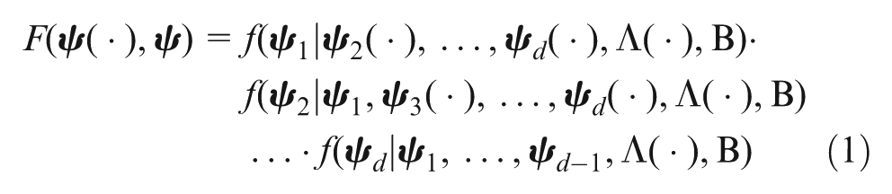
The joint distribution of $(ψ_{1} (i), \dots, ψ_{d} (i), Λ (i))$ converges to $f (ψ_{1}, \dots, ψ_{d}, Λ | B)$ when $i \to \infty$ .

In this case, there are 273 points as input point set, and the stationary objective function follows a Gaussian distribution. Based on Gibbs method, 1000 times interactive process is adopted, and the sampling random variables from Gaussian random numbers simulated the skin model as Figure 1.

Figure 1.

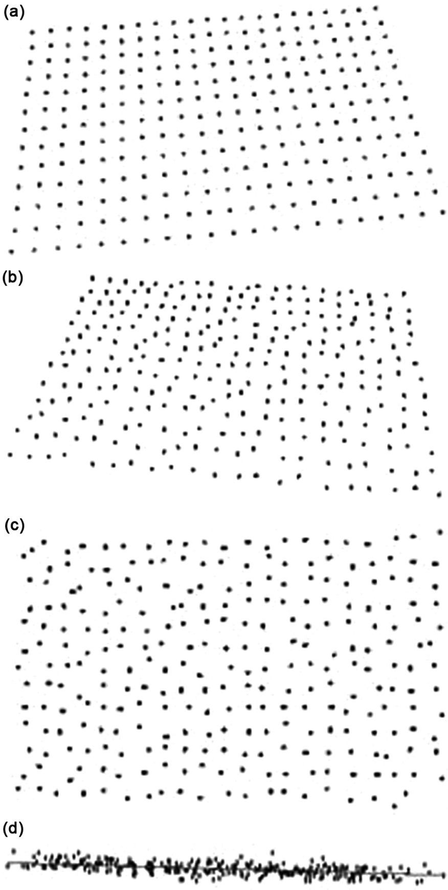
Skin model simulation by Gibbs method: (a) nominal model; (b) skin model view 1; (c) skin model view 2; and (d) skin model view 3.

Global approach

The skin model should satisfy tolerance specifications associated to the relevant nominal model. It means that the simulated skin model should be within the corresponding tolerance zone. Here, three types of geometric tolerances are considered: form tolerance, orientation tolerance, and position tolerance. After creating the random point set to simulate the skin model, the authors also intend to add geometric dimensioning and tolerancing constraints on it to satisfy the specification requirements. In order to simulate the skin model within a given tolerance zone, the direction of the tolerance zone should be determined first. For this purpose, a global model approach based on PCA is developed here.

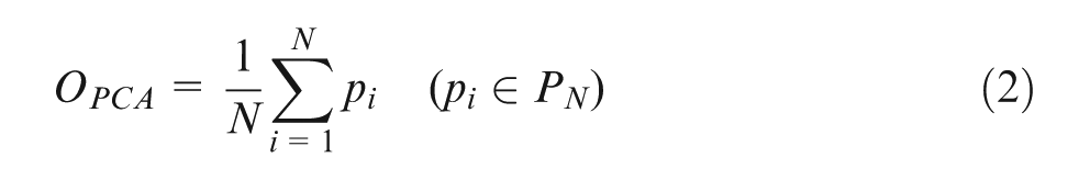
The PCA is a mathematical method used to convert a set of correlated variables into a set of values of uncorrelated variables called principal components.²⁷ It is usually used to evaluate the main element or structure of a set of data. Based on the covariance matrix, the PCA method proceeds in such a way that the first principal component has the highest variance (i.e. accounts for all the variability in a data set), and each succeeding component in turn has the highest possible variance within the constraint.

Consider a discrete shape $P_{N}$ represented by an arbitrary set of points $P_{i} = [x_{i}, y_{i}, z_{i}]^{T}$ . The PCA method computes the principal axes of the discrete shape using the following three steps:

(a) The origin of the principal coordinate system is determined as the centroid of $P_{N}$ that is calculated by

O_{PCA} = \frac{1}{N} \sum_{i = 1}^{N} p_{i} (p_{i} \in P_{N})

(2)

(b) The covariance matrix is defined by the following equation

M_{cov} = \sum_{i = 1}^{N} (p_{i} - O_{P C A}) {(p_{i} - O_{P C A})}^{T} (p_{i} \in P_{N})

(3)

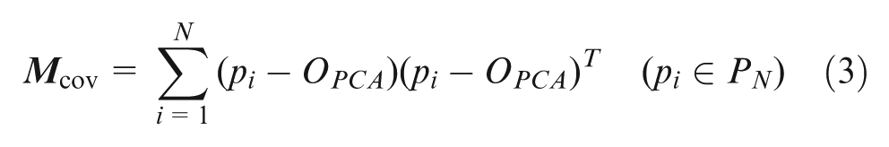
(c) The eigenvalues and eigenvectors can be calculated. The first principal axis is the eigenvector corresponding to the largest eigenvalue. The two other principal axes are obtained from the remaining eigenvectors.

In the following, a case study with flatness specification (form tolerance) is discussed to illustrate the method for skin model simulation considering the tolerance constraints.

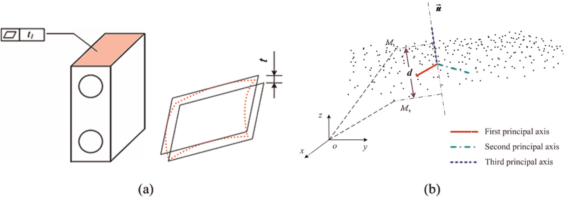
In Figure 2(b), the point set is a skin model of a plane that follows the Gaussian distribution. Using PCA method, the principal axis in three-dimensional space is evaluated. The direction of the third principal axis $\vec{n}$ is deemed as the tolerance zone direction. The skin model can be generated within the tolerance zone according to the tolerance zone direction. The constraints of orientation and/or position tolerances can be treated in a similar way.

Figure 2.

Skin model simulation with flatness specification: (a) the case with flatness tolerance and (b) flatness constraint.

Local approach

The “Global approach” section discussed the skin model simulation considering random deviations from a global perspective. Different from random errors that are statistical fluctuations, systematic deviations are reproducible. They usually follow recognizable signatures that can be calculated or simulated. In skin model shaping, it is thus reasonable to define some basic shape models (e.g. second-order shapes) to simulate those systematic errors.²⁸

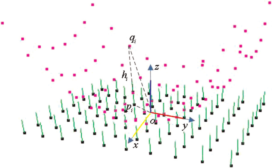
The augmented Darboux frame described the orientation, principal curvatures, and directions at a point on a surface²⁹ can be used as a local representation for a surface at each sample point. Let $p$ be a sampled point. The origin of a local frame is defined at $p$ . One of its axes is aligned with the surface normal at $p$ . The other two axes are aligned with the principal curvature directions at $p$ for which the normal curvature takes on maximum and minimum values, $k_{max}$ and $k_{min}$ . The five previous parameters when grouped as a system are often referred to as the augmented Darboux frame at $p$ . The discrete surface can be studied locally as a Monge patch, a height function $z$ of two spatial variables $x$ and $y$ defined using the augmented Darboux frame at $p$ . The local shapes for Monge patches are usually approximated as quadric shapes.

Kurokawa and Ariura²⁸ mathematically proved that an arbitrary second-order surface can be transformed into a fundamental form of the second order by the combination of rotation, translation, and scaling transformations. Based on this argument and augmented Darboux frames, the authors propose to model here the systematic deviations as one or a combination of some basic second-order surfaces or quadric shapes.

Systematic deviations simulation

The authors propose here the use of second order–form deviations to simulate the systematic deviations, since the second order–form deviations can reflect the principle curvature and the anisotropy of complex shapes better than the first-order and higher-order deviations.²⁸

For a plane, the common possible shapes considering the systematic deviations include: paraboloid, cone, sphere, cylinder, and ellipsoid. The morphing operation is a combination of a pure morphing, translation, and rotation of these basic shapes.

As an example, a paraboloid surface is simulated from the discrete model of a plane. The principle of our method can be explained by Figure 3, in which $S_{p}$ denotes the paraboloid point set and $I_{p}$ denotes the initial planar point set. The PCA algorithm is used to evaluate the principal axis to obtain the local coordinate system. Suppose $p_{i}$ is a random point of $I_{p}$ and $q_{i}$ is its corresponding point of $S_{p}$ .

Figure 3.

Paraboloid morphing method for planar shape.

The distance between these two points in $p_{i}$ s vertex normal direction is reflected using $h_{i}$ .

SSA

The SSA is commonly used for variability considerations in computer graphics, image processing, and bioinformatics domains.³⁰ The basic idea of this method is to establish a training set. The pattern of product geometric variation and the spatial relationships of structures are in a given class of shapes. Statistical analysis is used to give an efficient parameterization of this variability and to provide a compact representation of shapes.

To establish a statistical shape model, the following four steps are needed:³¹

Acquiring a training set from observation shapes;

Determining the correspondence of the observation shapes;

Aligning the training set through registration operations;

Analyzing the principal components and establishing the statistical shape models.

Suppose that a collection of $n$ discrete shapes (skin models) noted as $X_{1}, X_{2}, \dots, X_{n}$ is available. Where $X_{i}$ is a $d$ dimension vector, and $d$ is equal to the number of points composed the skin model. Since the skin model is calculated in the vector space, one may compute directly the empirical mean model using the method presented in Durrleman et al.,³¹ as in equation (4)

\bar{X} = \frac{1}{n} \sum_{i = 1}^{n} X_{i}

(4)

The covariance of this collection of skin models can be calculated by the following equation

\sum_{X} = \frac{1}{n} {\sum_{i = 1}^{n} (X_{i} - \bar{X}) (X_{i} - \bar{X})}^{T}

(5)

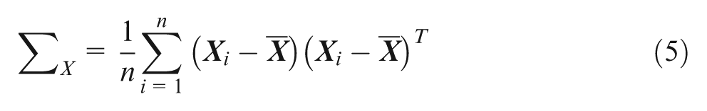
The covariance matrix $\sum_{X}$ is a $d \times d$ dimension matrix. The eigenvalue $(λ_{0}, λ_{1}, \dots, λ_{n - 1})$ and eigenvector $(ω_{0}, ω_{1}, \dots, ω_{n - 1})$ of the covariance matrix $\sum_{X}$ can be calculated. The principal components can be reflected by the eigenvector of covariance matrix $\sum_{X}$ . Let $W = [ω_{0}, ω_{1}, \dots, ω_{n - 1}]$ , the equation $\sum_{X} W = W Λ_{X}$ can be calculated. The diagonal matrix $Λ_{X}$ can be described as follows

Λ_{X} = (\begin{matrix} λ_{1} & 0 \\ ⋱ \\ 0 & λ_{d - 1} \end{matrix})

(6)

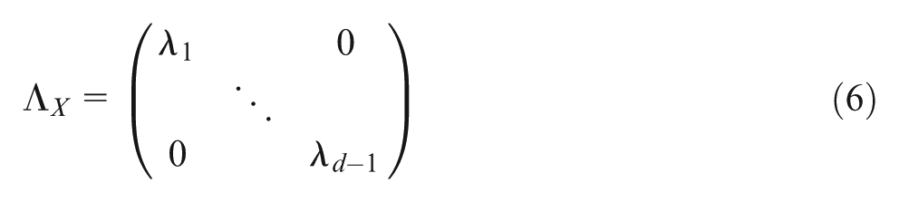
The eigenvalues reflect the variance of the principal components. When the principal component has a bigger eigenvalue, it reserves more information of an initial sample. In our method, the principal components with bigger eigenvalues are selected to simulate the initial sample vector. The first $t (t < d)$ maximal eigenvalue fulfills the following equation

\sum_{k = 0}^{t} λ_{k} / \sum_{k = 0}^{d - 1} λ_{k} \leq ε

(7)

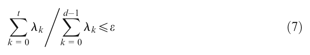
Let $W_{X} = [ω_{0}, ω_{1}, \dots, ω_{t - 1}]$ , then each vector of the sample data can be described by the following equation

X \approx \bar{X} + W_{x} b_{x}

(8)

where $\bar{X}$ is the mean. The $t$ -dimensional vector $b_{x}$ is the shape coefficient that controls the models of variation.

The main function of statistical shape model is to determine the mean model among numerous sampling shape models and to predict new shape model belonging to the same shape family. Since $\bar{X}$ and $W_{x}$ are invariants in a training set, the various shape models are obtained and determined by $b_{x}$ . Under Gaussian distribution assumptions, it can be calculated using equation (9)

b_{x} = \pm 3 \sqrt{λ_{i}} (i = 0, 1, …, t - 1)

(9)

Case study

The case study is based on a sheet metal part manufactured in a one-stage sheet metal forming process. The manufacturing process is simulated using stochastic finite element (FE) techniques. The tooling is modeled as rigid parts and a process macro is used to define the processes, such as stamping velocity, blank holder force, and friction. An initial model of the stamping process is served as a basis for the variation of process parameters. The selected variables (e.g. blank thickness, drawing depth, punch radius, die radius, and flange width) are computed using Latin hypercube sampling under the assumption of the independence of the variables and normal distributions.³² The manufactured cross-shaped parts was measured using ATOS-Ifringe projection system. Figure 4 shows the CAD model of the cross-shaped part and its geometric specifications.

Figure 4.

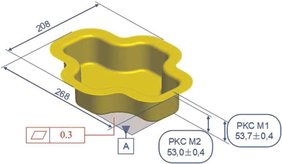
The cross-shaped part.

Skin model simulation

In this case, the simulation method of the skin model of a bottom plane with flatness specification constraints is considered. Based on the CAD model (Figure 5), the bottom plane can be extracted using CATIA V5 generative shape design (GSD) utilities as illustrated in Figure 6.

Figure 5.

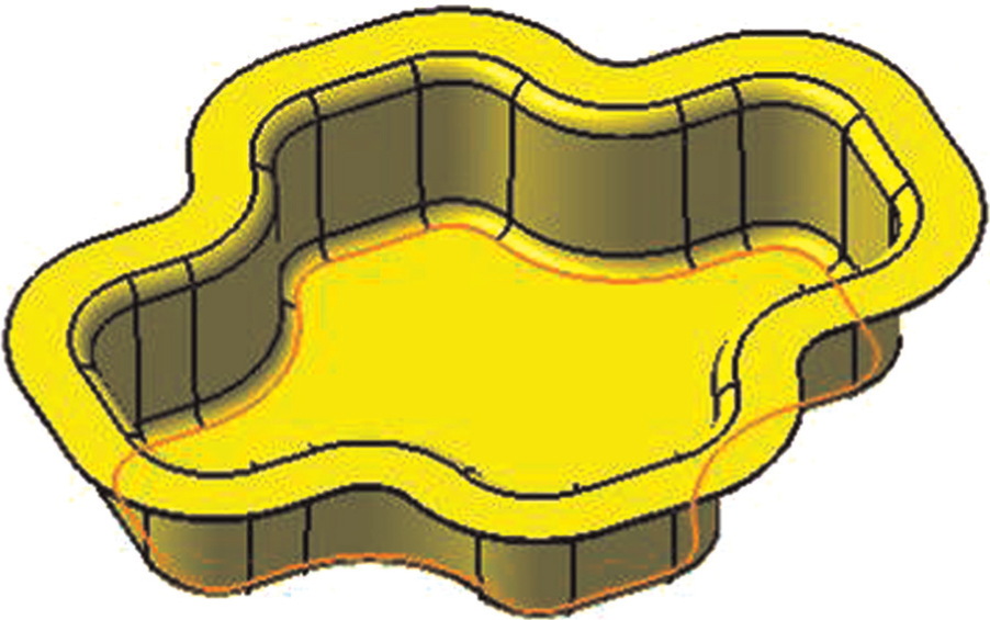
Segmentation of the computer-aided design model.

Figure 6.

Bottom plane extraction.

In order to discretize the bottom plane, a tessellation operation is implemented using CATIA V5 software. Figure 7 illustrates the tessellation result composed of 2392 points and 4550 facets.

Figure 7.

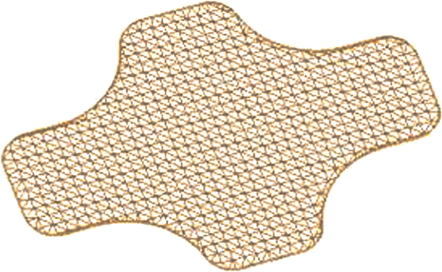
Tessellation of the bottom plane.

Based on the tessellated CAD model and the geometric specification of flatness, different skin models can be generated using the methods discussed in the “Skin model simulation” section. In this case, we create skin models of the bottom plane by Gibbs method with flatness equals to 0.3 mm.

However, based on the information from measurement and simulation data, the skin model can be improved considering both systematic and random errors. The analysis of this measurement point set is illustrated in Figure 8.

Figure 8.

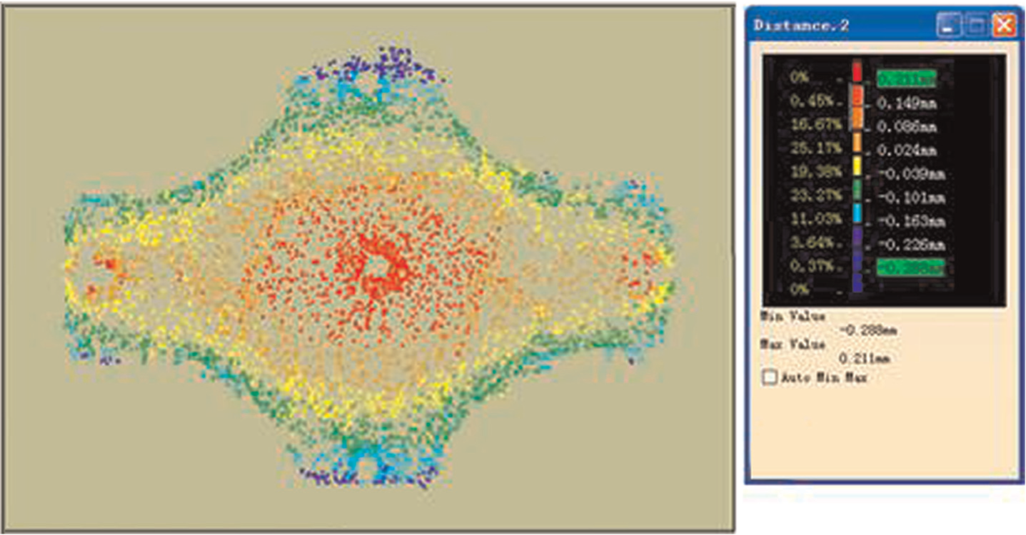
Analysis of measured point data of cross-shaped part.

Based on the nominal discrete bottom plane model (Figure 7), the skin model with ellipsoid systematic deviations is simulated (see Figure 9). To visualize the deviations clearly, the limited deviations are reflected by red and blue colors.

Figure 9.

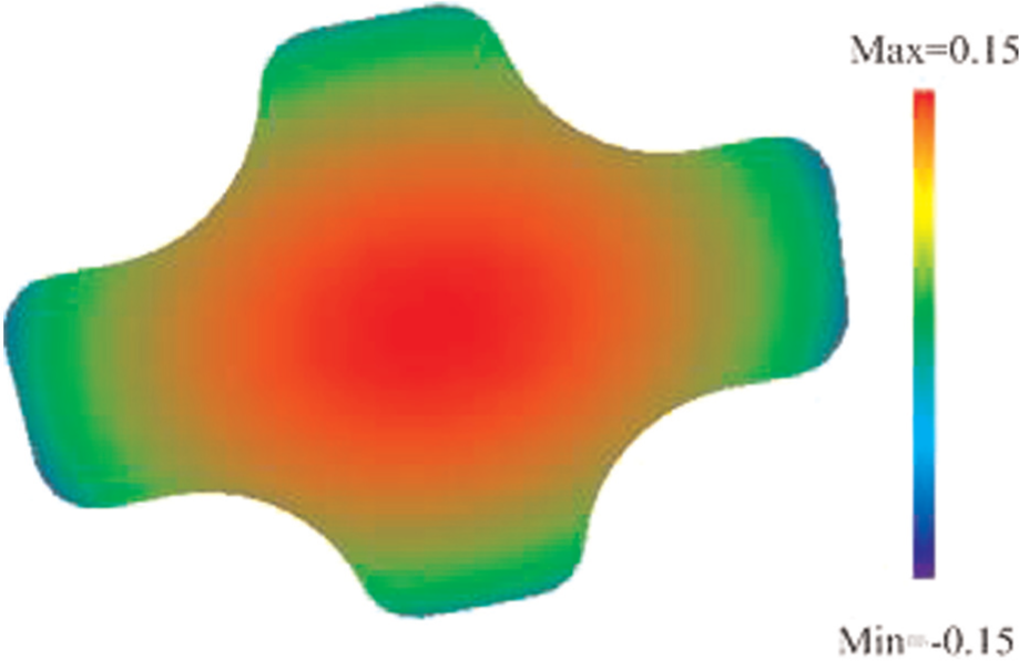
Visualization of systematic deviations.

Random errors are added to the skin model with ellipsoid systematic errors. The Gibbs method is adopted to simulate the random errors. The skin model with both systematic errors (ellipsoid) and random errors (Gaussian distribution) is created. The representation of the skin model is refined using a color-scale technique (see Figure 10). It shows that the form deviations consider both the ellipsoid shape variety and Gaussian random noises.

Figure 10.

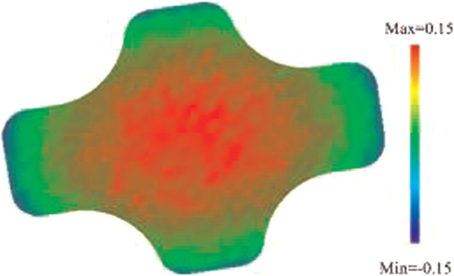
Color scale of skin model with both systematic and random errors.

Statistical shape modeling

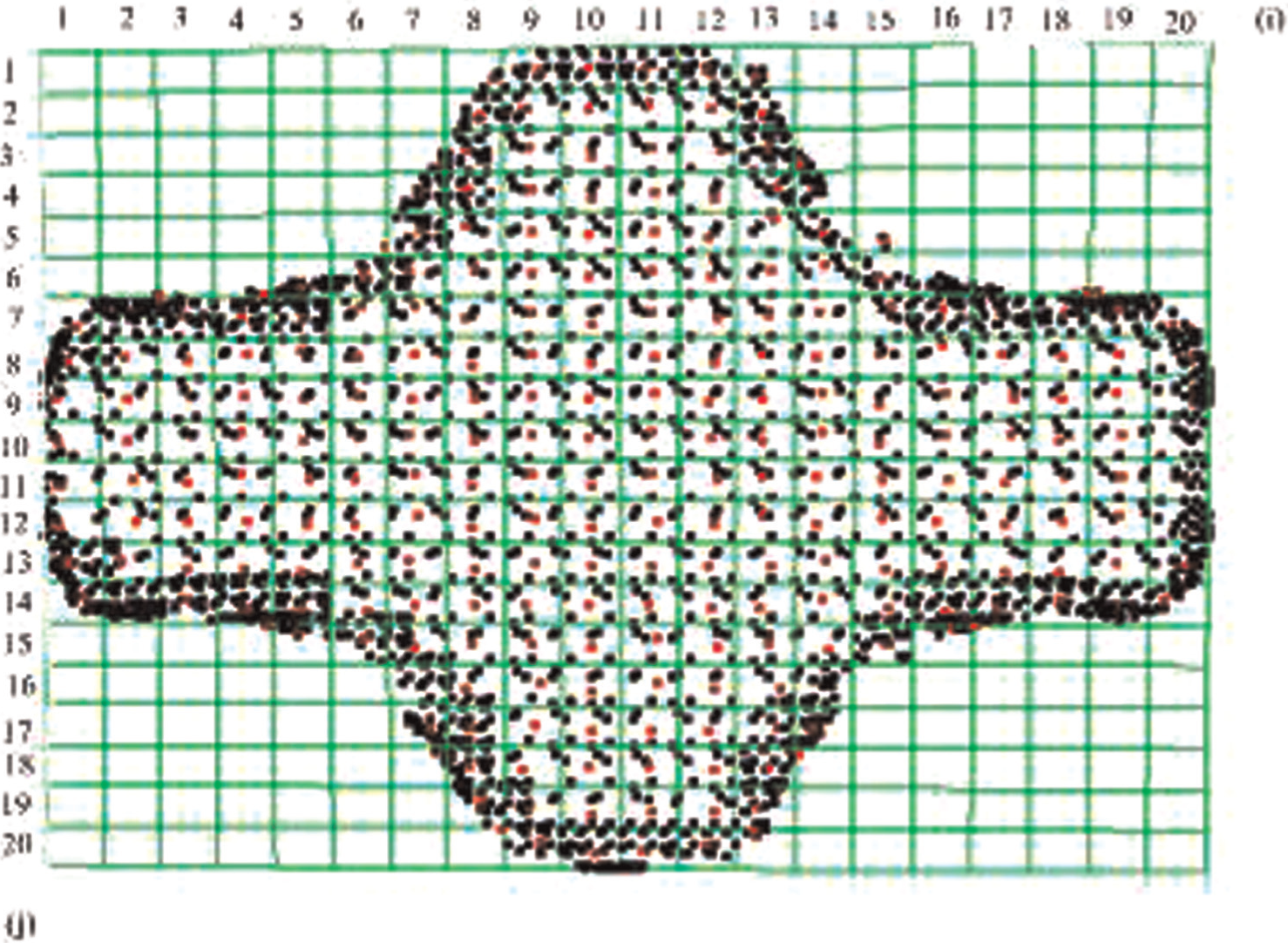
To calculate the mean model considered in the manufacturing process, a training set is designed with 10 models obtained using FE analysis (FEA) method.³² The relationships among these 10 samples are established by landmark techniques. In our case, each landmark corresponds to a unique grid marked as $(i, j)$ . The mean point $p$ is served as a center of a corresponding grid (see Figure 11).

Figure 11.

Landmarks arrangement.

Based on the dimensional scale and the coordinate reference system of the FEA technique, all the samples are aligned using the registration algorithm. Figure 12 shows the positions of all the samples reflected by a different color.

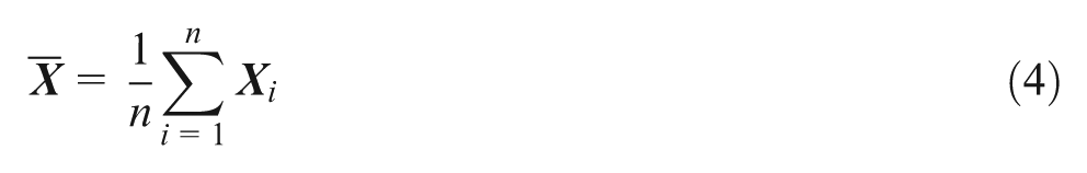
After aligning the samples, the mean model can be calculated using equation (4). Using the same process, the mean model of the training set can be obtained. These samples are simulated by the approach proposed in the “Skin model simulation” section.

Figure 12.

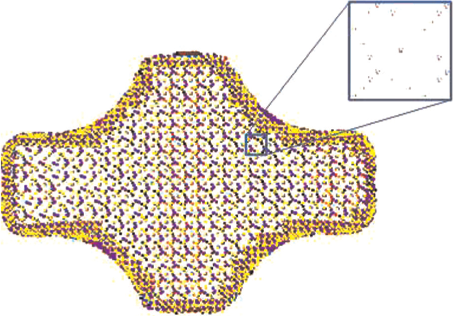
Alignment of the training set.

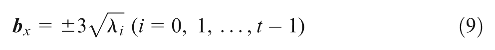
Based on the PCA technique, the deviation between the mean model and each sample can be calculated using equation (5). The influence of each component can be deduced. According to the different kinds of mean models, the new skin models can be predicted based on equation (9) (Figure 13). This process is able to enrich the property of skin model, which can combine information from different design means, even manufacturing and inspection domains.

Figure 13.

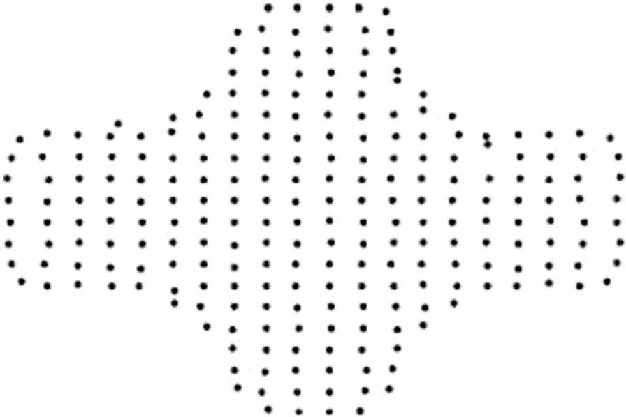
Predicted skin model with $b_{1} = - 2 \sqrt{λ_{1}}$ .

Conclusion

Skin model simulation is one of the most critical issues in GPS and GeoSpelling domain. This article proposed to develop methods to shape the skin models with random and systematic deviations. Based on the hypothesis that the random deviations follow the normal distribution, the MCMC method is developed to generate the skin models with discrete representations. A new skin model simulation method combined both a global-modeling approach based on PCA, and a local-modeling approach based on augmented Darboux frame is considered. The local–global modeling approach enables the simulation of both random and systematic deviations when considering geometric constraint requirements, tolerance specifications, and manufacturing. In addition to discrete shape modeling for skin model representation and simulation, the concept of the mean skin model and its robust statistics are also introduced in this work. A new method based on statistic shape models is developed for skin model simulation and analysis. The contribution of this study to the industry is that it can enrich skin models with different influencing factors (such as temperatures, materials, stress, etc.).

Using a case study based on a cross-shaped sheet metal part, the results of the skin model simulations and statistical analysis are shown, and the performances of the simulations are discussed. The obtained results show the performance of this new approach.

Footnotes

Funding

The authors would like to thank China Scholarship Council (CSC) for its research funding.

References

Srinivasan

. Mathematical theory of dimensioning and parameterising product geometry. Int J Prod Lifecycle Manag 2005; 1(1): 70–85.

Hans-Jürgen

. Evaluation of uncertainty in measurements—problems and tools. Opt Laser Eng 2002; 38(3–4): 185–206.

Dantan

Anwer

Mathieu

. Integrated tolerancing process for conceptual design. CIRP Ann Manuf Techn 2003; 52(1): 135–138.

Hillyard

Braid

. Analysis of dimensions and tolerances in computer-aided mechanical design. Comput Aided Design 1978; 10(3): 161–166.

Requicha

AAG

. Representation of tolerances in solid modeling: issues and alternative approaches. New York: Plenum Publishing Corporation Press, 1984, pp.3–22.

Bourdet

. Contribution a la Mesure Tridimensionnelle: Modele d’ideentification des surfaces, Metrologie fonctionnelle des pieces mecanniques, correction geometrique des machines a mesurer tridimentionnelles. These d’Etat, Nancy, France, 1987.

Jayaraman

Srinivasan

. Geometric tolerancing I: virtual boundary requirement. IBM J Res Dev 1989; 33(2): 90–104.

Srinivasan

Jayaraman

. Geometric tolerancing II: conditional tolerance. IBM J Res Dev 1989; 33(2): 105–122.

Etesami

. Mathematical model for geometric tolerances. J Mech Design 1993; 115(2): 81–86.

10.

Shah

Yan

Zhang

. Dimension and tolerance modeling and transformations in feature based design and manufacturing. J Intell Manuf 1998; 9(5): 475–488.

11.

Roy

Sudarsan

Sriram

. Information models for Design Tolerancing: From Conceptual to the Detail Design, ASME, DETC99 Conference, Las Vegas, Nevada, September, 1999.

12.

Ballu

Mathieu

. Univocal expression of functional and geometrical tolerances for design, manufacturing and inspection. In: Proceedings of the 4th CIRP seminar on computer aided tolerancing, 4th CIRP Seminar, Tokyo, Japan, April 5–6, 1995; London: Chapman & Hall, 1996, pp.31–46.

13.

ISO 17450-1. Geometrical product specifications (GPS)—general concepts—part 1: model for geometrical specification and verification, 2005.

14.

. Study on the theories and methods of functional tolerancing based on new GPS. PhD Thesis, Zhejiang University, China, 2008.

15.

Naylor

. Computational representations of geometry, SIGGRAPH’96 Course Notes, 1996.

16.

Shapird

. Solid modeling. Technical Report, University of Wisconsin—Madison, Madison, WI, 2001.

17.

Johnson

. Dimensioning and Tolerancing, Final Report, R84-GM-02-2, CAM-I. Arlington, TX, 1985; Computer Aided Manufacturing-International, 1985.

18.

Requicha

AAG

Chan

. Representation of geometric features, tolerances and attributes in solid modelers based on constructive solid geometry. IEEE J Robot Autom 1986; 2(3): 156–165.

19.

Gossard

Zuffante

Sakurai

. Representing dimensions, tolerances and features in MCAE systems. IEEE Comput Graph 1988; 22(1): 51–59.

20.

Zhang

Anwer

Mathieu

. A unified geometrical product specification and verification model interpreted by discrete geometry. In: Proceedings of the IDMME virtual concept international conference, Bordeaux, France, October 20–22 2010.

21.

Kurfess

Banks

. Statistical verification of part geometry. Comput Aided Design 1995; 27(5): 353–361.

22.

Yang

Jackman

. Form error estimation using spatial statistics. J Manuf Sci E: T ASME 2000; 122: 262–272.

23.

Samper

Formosa

. Form defects tolerancing by natural modes analysis. J Comput Inf Sci Eng 2007; 7: 44–51.

24.

Caskey

Hari

Hocken

. Sampling techniques for coordinate measuring machines. In: Design and manufacturing systems conference, January 9–11, 1990; Austin, TX, 1991, pp.779–786.

25.

Zhang

Anwer

Mathieu

. A discrete geometry framework for geometrical product specifications. In: Proceedings of the 21st CIRP design conference, Kaist, Korea, March 27–29, 2011, pp.142–148.

26.

Wang

. Simplified engineering mold of normal distribution function. Mech Res Appl 2007; 20(2): 31–36.

27.

Pearson

. On lines and planes of closest fit to systems of points in space. Philos Mag 1901; 6(2): 559–572.

28.

Kurokawa

Ariura

. Evaluation of shot penned surfaces using characterization technique of three-dimensional surface topography. J Phys Conf Ser 2005; 13: 9–12.

29.

Ferrie

Lagarde

Whaite

. Darboux frames, snakes, and super-quadrics: geometry from the bottom up. IEEE T Pattern Anal 1993; 15(8): 771–783.

30.

Cootes

Taylor

. Statistical models of appearance for medical image analysis and computer vision. In: Proceedings of the SPIE medical imaging, San Diego, CA, February 17–22, 2001; In image Processing, pp.236–248.

31.

Durrleman

Pennec

Trouvé

. Statistical models on sets of curves and surfaces based on currents. Med Image Anal 2009; 13(5): 793–808.

32.

Stockinger

Wittmann

Martinek

. Virtual assembly analysis: standard tolerance analysis compared to manufacturing simulation and relative positioning. In: Proceedings of the 11th international design conference DESIGN, Dubrovnik, Croatia, May 17–20, 2010, pp.1421–1430.

Discrete shape modeling for skin model representation

Abstract

Keywords

Introduction

Skin model simulation

Random deviation simulation based on MCMC

Global approach

Local approach

Systematic deviations simulation

SSA

Case study

Skin model simulation

Statistical shape modeling

Conclusion

Footnotes

Funding

References