
Abstract
Point grinding is a cylindrical grinding process where the grinding wheel axis can be tilted relative to the workpiece axis by a swivel angle to yield a point contact. This feature enables complex parts to be ground in a single set-up on a point grinding machine. In this article, the effect of the swivel angle on the workpiece surface finish was investigated experimentally and numerically for different workpiece materials. There was good agreement between the measured and predicted workpiece surface roughness values Ra with an average difference of 6.3% for the three cutting speeds tested. It was also observed that, for the grinding conditions investigated, the swivel angle does not significantly influence the resulting workpiece surface roughness.
Introduction
Point grinding is a variation of cylindrical grinding used to grind complex cylindrical shapes with a thin superabrasive wheel at high speeds. As described by Koepfer 1 and shown in Figure 1, point grinding involves tilting the axis of rotation of the grinding wheel by a swivel angle α with respect to the workpiece axis. The wheel and workpiece rotate with speeds v s and v w , respectively, as the grinding wheel is fed into the workpiece at a rate of v f . Since the workpiece and grinding wheel axes are skewed, the final workpiece surface is generated at a point rather than a line as in conventional cylindrical grinding. This fact, along with the narrow wheel, makes it possible to grind shapes that are more complex than can be ground using conventional cylindrical grinding operations in one set-up. Example shapes include: tapered contours, plunge cuts, shoulders, and slots. The swivel angle also has the effect of reducing the contact length, which affects the grinding mechanics. Xiu and Cai 2 showed how the basic geometrical grinding parameters, such as contact length, cutting depth, and uncut chip thickness, were influenced by the swivel angle. To the present authors’ knowledge, no publications exist that study the effect that swivel angle has on the resulting workpiece surface finish; therefore, this article will investigate this effect using both simulation and experimentation.
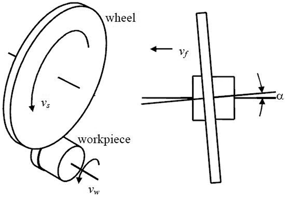
Layout of point grinding.
Simulation method
The authors of this article developed a simulation tool that would complement their experimental investigations of surface finish in point grinding. One of the key criteria for this simulation software was that it runs on a desktop computer in a reasonable amount of time. To meet these criteria, the authors decided to simulate only the geometric aspects of grinding metal removal and ignore the physics of the problem. One way of simulating the geometry of metal removal is to create a model of the cutting edges and a model of the workpiece and use Boolean subtractions to mimic metal removal. This method can provide useful information about the grinding process itself; for instance, this approach can calculate the uncut chip thickness that may be helpful in understanding the mechanics of the process. The disadvantage of this method is that it requires significant computational resources to perform the myriad Boolean subtractions. In the case of grinding, these types of simulations need to be executed on clusters of computers, rather than on a single desktop computer.
In this article, the approach to simulating metal removal was based on the work by Nguyen and Butler.3,4 This approach does not use Boolean subtractions but, instead, combines the trajectories of individual cutting edges to form the final workpiece surface finish. This method has the advantage of being more computationally efficient than methods that use Boolean subtractions; however, it does not enable calculations of the uncut chip thickness. In this article the method proposed by Nguyen and Butler has been modified in the following two ways. Nguyen and Butler approximated the trajectories of the cutting edges as parabolic curves while, in the present work, the exact trochoidal trajectories of the cutting edges were used. The other difference is that Nguyen and Butler applied their technique to surface grinding while, in the present work, the technique was applied to cylindrical point grinding.
In this research, the cutting edges are modeled as points on the circumference of the wheel and the wheel itself is sectioned into n circular two-dimensional (2D) slices. One of these circular slices is illustrated in Figure 2 where it is shown that the position of each cutting edge in a given slice can be defined by its effective radial distance from the center of the wheel r i and its angle θ i as measured in a counter-clockwise direction from bottom dead center.
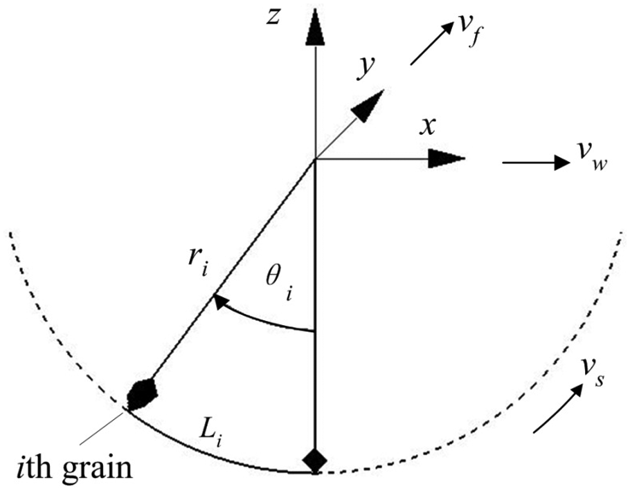
Grinding wheel geometry and kinematics.
Note that an effective radius r i is used to combine the workpiece and wheel radii into one parameter

where r s is the distance from the wheel center to the cutting edge and r w is the workpiece radius. The motion of each cutting edge has two components: a rotation about the center of the wheel v s /r i and a translation in the horizontal direction v w . Together, this geometry and motion can be expressed parametrically for a single cutting edge as
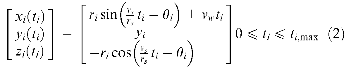
where
These time-dependent trajectories can be mapped onto the spatial coordinates of the workpiece surface by solving numerically for the time when a cutting edge is at a given x-coordinate along the workpiece surface
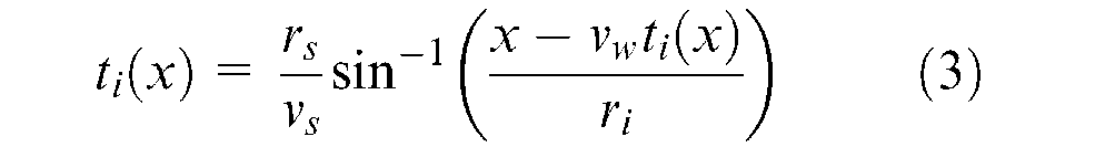
In general there will be several solutions to equation (3). Since it is only the portion of the grain trajectory that has the potential to generate the finished workpiece surface that is of interest, the value of
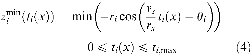
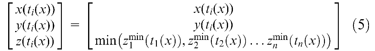
The resulting planar trajectories of four cutting edges are illustrated in Figure 3. As can be seen in this figure, the trajectories of the four cutting edges overlap. The unwanted portions of the grain trajectories are removed by comparing the z-coordinates of all the trajectories at a particular x-location along the workpiece surface and constructing a surface by only using the point corresponding to the minimum z-coordinate
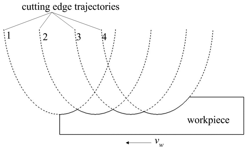
Selection of four cutting edge trajectories.
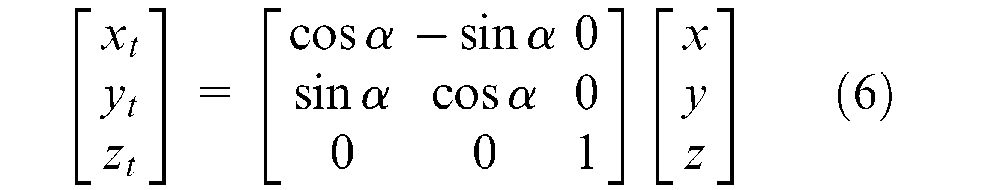
Once a point on the workpiece surface is calculated, the swivel angle α that is offered by point grinding can be taken into account using the following rotation about the z-axis
Lastly, the 2D traces within each of the n slices are assembled into the three-dimensional (3D) finished workpiece surface as shown in Figure 4.
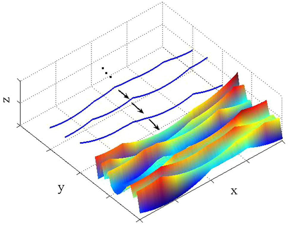
Generation mechanism of workpiece surface.
Wheel model
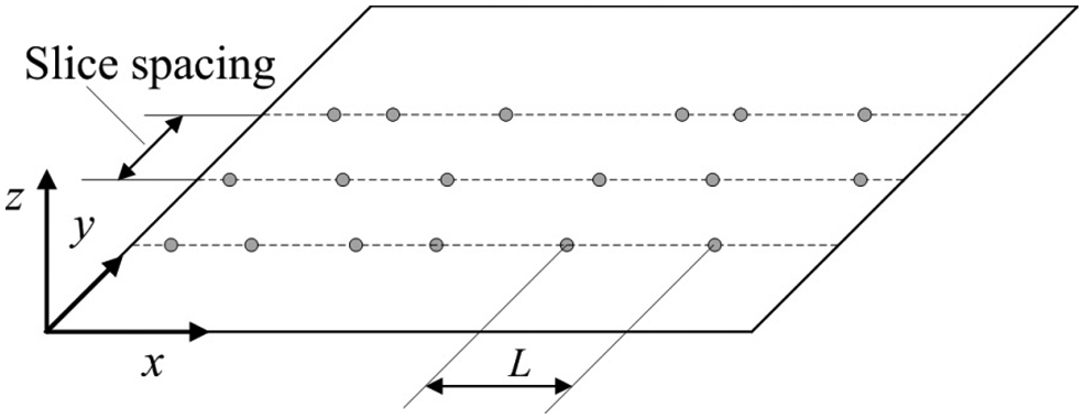
The most important characteristics of the cutting edges on a grinding wheel are: the protrusion height of the grains (which is the distance between the cutting edge and the center of the wheel), the spacing of the grains along the circumference of the grinding wheel L as shown in Figure 5, and the size of the cutting edges as discussed in detail by Koshy et al. 5 and Doman et al. 6 According to Doman et al. 6 there is no conclusive experimental evidence supporting any particular distribution of these parameters. In this work it was assumed that the protrusion height of the active grains conforms to a normal distribution with the following probability density function
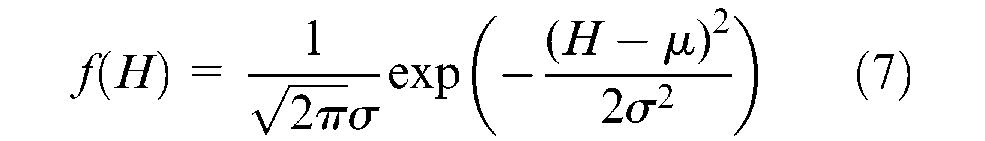
where H is the protrusion height of a grain measured from the effective wheel radius, and µ and σ are the mean values of the protrusion height and standard deviation, respectively.
Cutting edge spacing.
Given that the mean value of the protrusion height is the working surface of the grinding wheel (which is the effective wheel radius r i ), µ is equal to zero. The value of σ was based on the dressing parameters, as shown in Figure 6, because it is reasonable to assume that all active grains are dressed. From this figure one can see the conically shaped single-point dressing tool at two different positions – spaced by the dressing feed per revolution f d at a dressing depth a d . At this dressing depth, the active width of the tool is b d and the depth of the thread cut into the grinding wheel is A. From Figure 6, it is evident that the following relationship between these dressing parameters holds
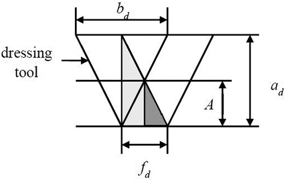
Dressing geometry.

Rearranging equation (8) yields

from which σ can be calculated.
According to Malkin and Guo, 7 the average and maximum grain that can pass through a sieve with a mesh size of M are


The resulting grain spacing was assumed to be a uniform distribution on the surface of the grinding wheel, and the probability density function
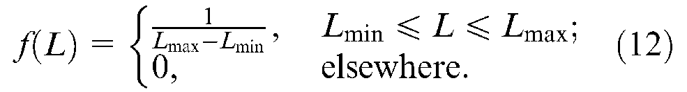
where Lmax and Lmin represent the maximum and minimum spacing between the adjacent grains along the wheel, respectively. The values for Lmax and Lmin were determined by considering the volume of abrasive grits V g in a grinding wheel. Given that the packing density G0 for a Cubic Boron Nitride (CBN) grinding wheel is expressed in terms of carats per cm3 (ct/cm3) and, according to Malkin and Guo, 7 the density of CBN in grinding wheels is 3.48 g/cm3, the resulting grain volume fraction V g can then be calculated as

If the grains are assumed to be arranged in a simple cubic packing structure, then there is a total of one grain per unit cell and

where

According to Marinesscu et al., 8 the cutting edge density C is

where
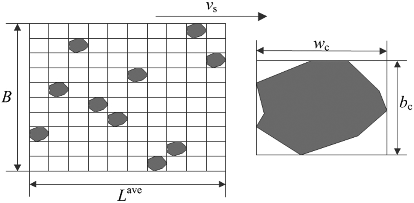
Cutting edge density.

Since there is only one grain per unit cell it follows that the cutting edge density is also

Combing equations (17) and (18) and solving for L yields

The value for Lmax is obtained by substituting
Experimental results
To validate the proposed numerical model, point grinding experiments were carried out on a super-high-speed cylindrical grinder (Figure 8) developed at Northeastern University in China, which can achieve cutting speeds of up to 150 m/s. These wet grinding experiments studied three different cutting speeds v s corresponding to 30, 60 and 90 m/s using a CBN grinding wheel (370 mm diameter × 6 mm width), which has a 125% concentration (5.5 ct/cm3) and 120 grit size. For each cutting speed v s , AISI 1045 (173 HB) workpieces of diameter 50 mm were ground using an axis feed rate v f of 0.5 mm/s, a workpiece speed v w of 0.1 m/s, a cutting depth a of 0.05 mm, and a swivel angle α of 0.5°. Single point dressing with a dressing depth of 0.012 mm and an overlap ratio of 1.8 was used to condition the wheel. The resulting workpiece surface topologies were then measured using a Sciences et Techniques Industrielles de la Lumière (STIL) Micromeasure 2 optical profilometer. Two experiments were carried out per cutting speed.
super-high-speed cylindrical grinder.
Point grinding numerical simulations were also carried out with the same grinding parameters used for the experiments. The predicted 3D workpiece surface topologies from these simulations can be compared with the experimentally measured workpiece surfaces in Figure 9 for each of the three cutting speeds tested. The lowest point in each 3D topology was used as a zero reference. While the simulation and experimental results appear to qualitatively look similar over the selected sample area, one can notice small spikes that appear on the measured surface that were not captured by the numerical model. These spikes are about 7.5 μm wide and 0.35 μm high and could be swarf, measurement noise, or plowed ridges caused by workpiece material flow during cutting.
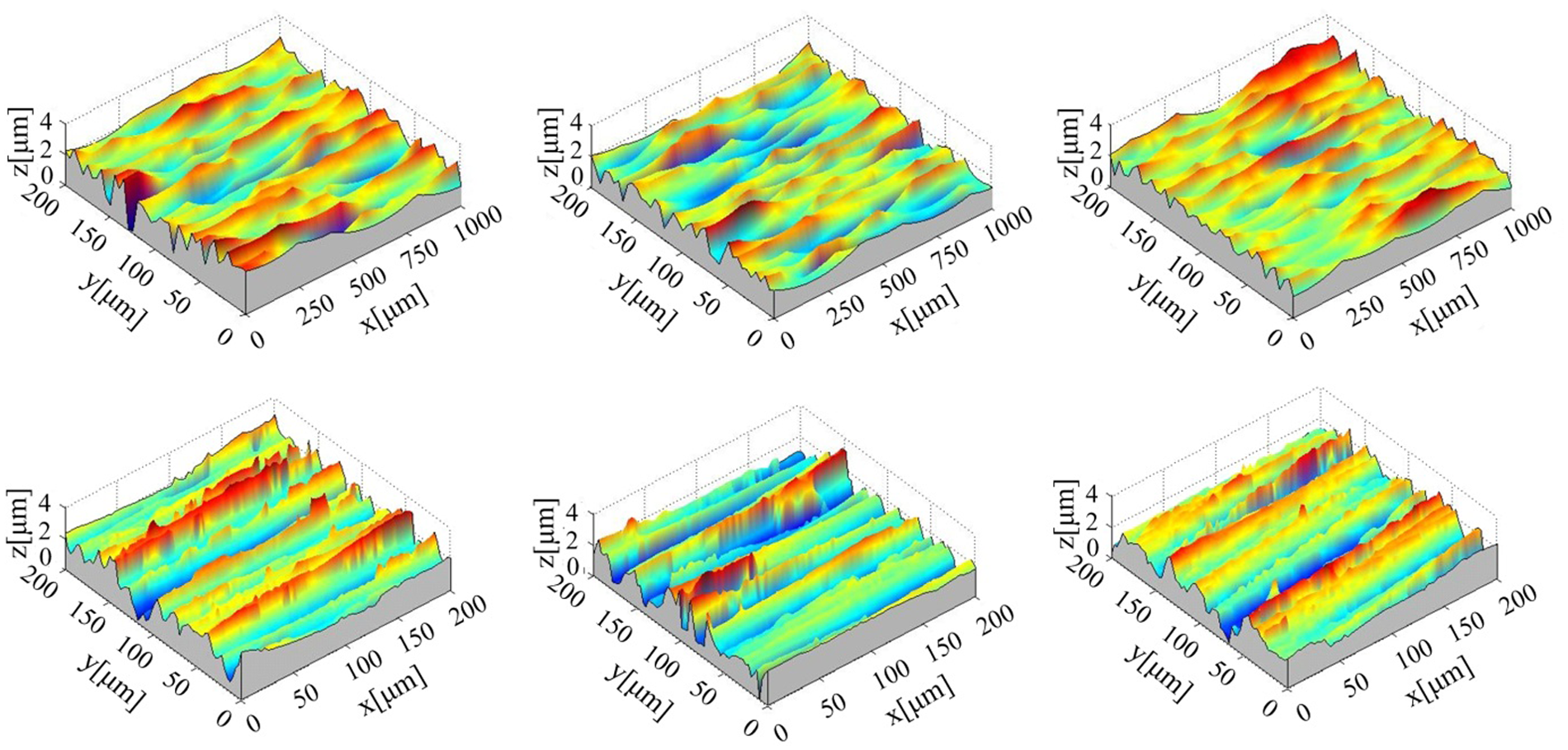
Workpiece topography: simulation (top) and experiment (bottom).
Sample simulated and experimental profiles taken perpendicular to the cutting direction are shown in Figure 10 for each of the three cutting speeds tested. It is evident that the heights of the peaks and valleys for both the simulated and experimental results are similar.
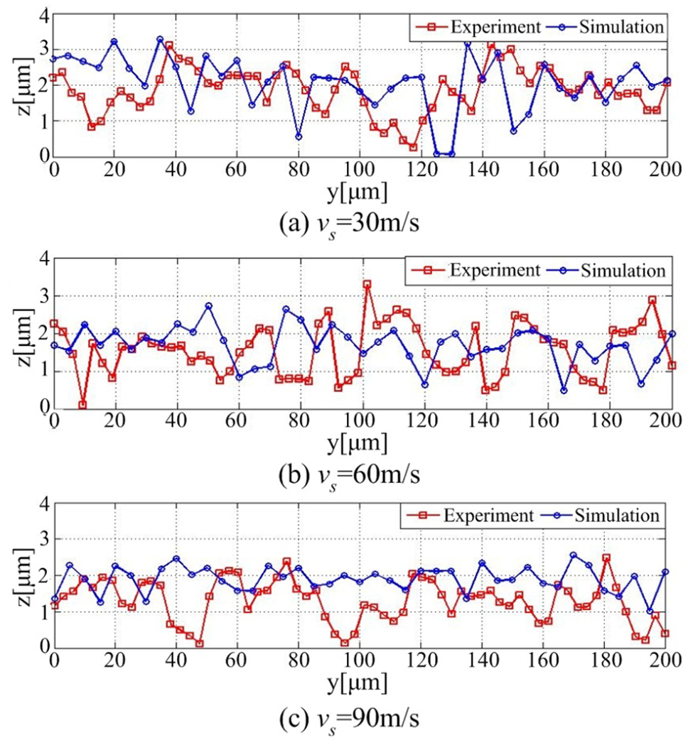
Cross section of workpiece surface.
To quantitatively compare these results, Figure 11 plots the corresponding arithmetic mean surface roughness Ra for all three cutting speeds. For each cutting speed, the experimentally measured maximum, minimum, and average roughness values are plotted, along with the predicted roughness values from the simulator. It can be seen that there is good agreement between the measured and predicted roughness values with an average difference of 6.3%. The simulator appears to slightly under-predict the experimental results. This observation is expected because the simulator does not capture effects such as machine vibrations, cutting mechanics, and chip adhesion, which would tend to produce a rougher workpiece surface. It can also be observed in Figure 11 that both the experimental and simulation results predict a slight decrease in the surface roughness as the cutting speed increases. This decrease in roughness can be attributed to an increase in the number of abrasive grains interacting with the workpiece as the cutting speed increases.
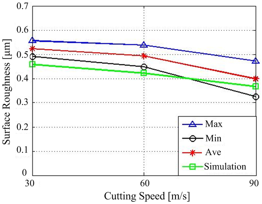
Relationship between surface roughness and cutting speed.
To further quantify the results, Figure 12 plots the simulated and experimental workpiece surface height distributions for each cutting speed tested. By plotting the percentage number of observations (frequency) of each height observed over the selected sample workpiece area, one can see that there is excellent agreement in height distributions between the predicted and measured workpiece topographies. At a cutting speed of 30 m/s, the average height distribution is 1.76 μm and 1.81 μm for the simulation and experimental results, respectively. Similarly, for cutting speeds of 60 m/s and 90 m/s, the average simulated height distributions are1.42 μm and 1.4 μm, respectively, while the average experimental height distributions are 1.46 μm and 1.43 μm, respectively. These results are consistent with Figure 11, where it was observed that the surface roughness decreases as cutting speed increases.
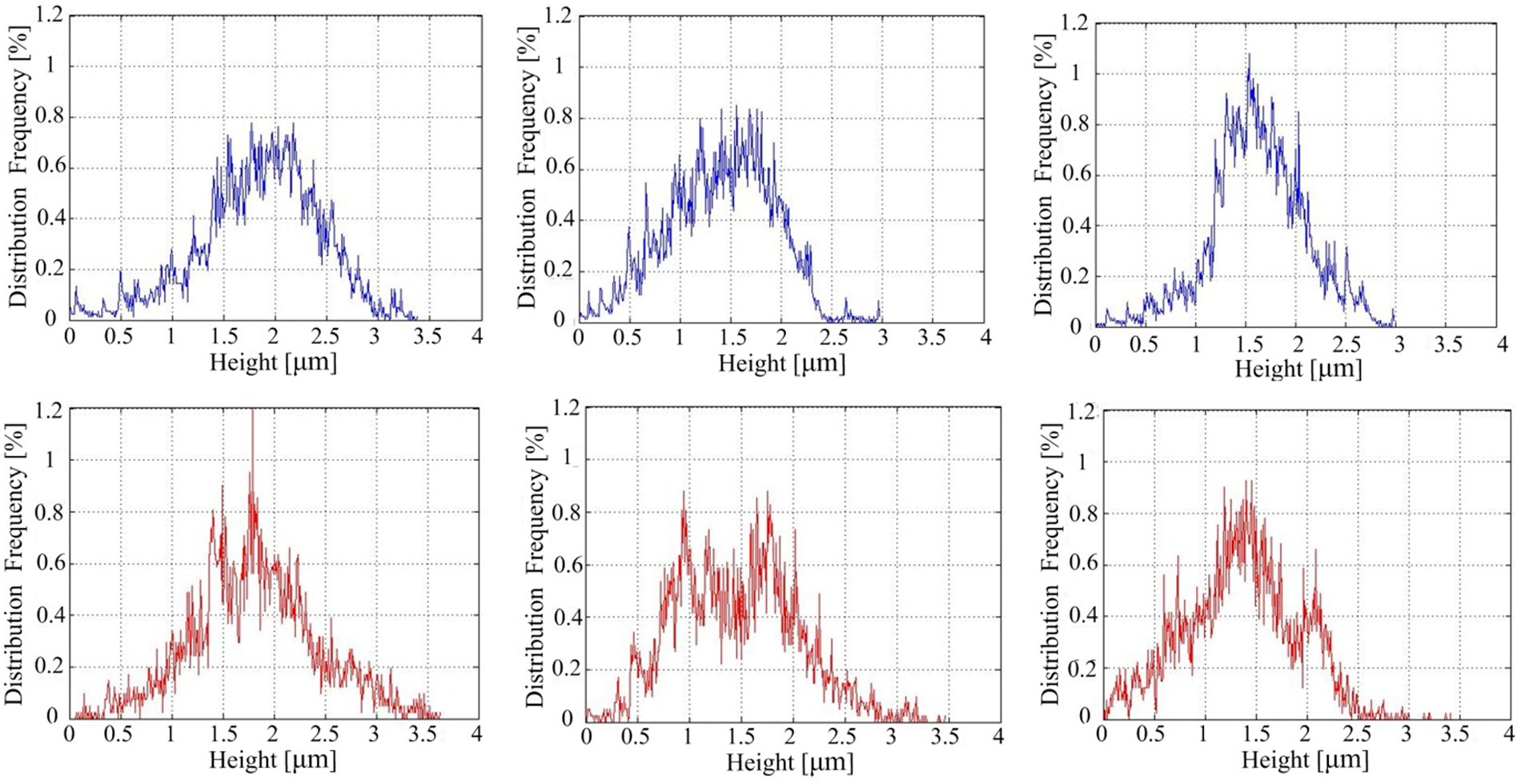
Height distribution frequency: simulation (top) and experiment (bottom).
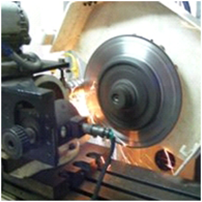
Next, a series of point grinding experiments were carried out with a MK9025 cylindrical grinder, as shown in Figure 13 (maximum cutting speed of 40 m/s), to study the effect the swivel angle α has on the resulting workpiece surface roughness. These dry grinding experiments used eight different swivel angles corresponding to 0, 0.5, 1, 1.5, 2, 2.5, 3, and 4 degrees. These experiments used a CBN grinding wheel (180 mm diameter × 10 mm width) having a 125% concentration (5.5 ct/cm3) and 120 grit size. For each swivel angle α, three different 50 mm diameter workpiece materials were tested: AISI 1045 steel (173 BH), AISI 5140 steel (165 BH), and GB 30CrMnSi structural alloy steel (220 GB). All other grinding conditions were held constant with an axis feed rate v f of 0.04 mm/s, a workpiece speed v w of 0.26 m/s, a cutting depth a of 0.03 mm, and a cutting speed v s of 35 m/s. Single point diamond dressing, with a dressing depth of 0.02 mm and overlap ratio of 2.1, was used to condition the wheel and, to ensure repeatability of the results, each experiment was carried out five times. The results presented in this research represent the average of the five repeatability tests. The resulting workpiece surface topologies were then measured using the same STIL Micromeasure 2 optical profilometer used in the previous set of experiments.
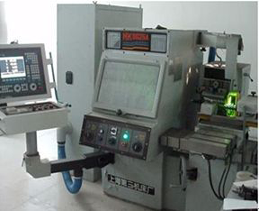
MK9025 cylindrical grinder.
Figure 14 plots the corresponding measured workpiece surface roughness Ra as a function of swivel angle for each of the three materials tested. Superimposed on this figure are the predicted roughness values from computer simulations that were carried out under the same point grinding conditions. This figure confirms that that both the experimental and simulation results suggest that there is no significant relationship between surface roughness and the swivel angle for angles less than four degrees, even when the workpiece material is changed.
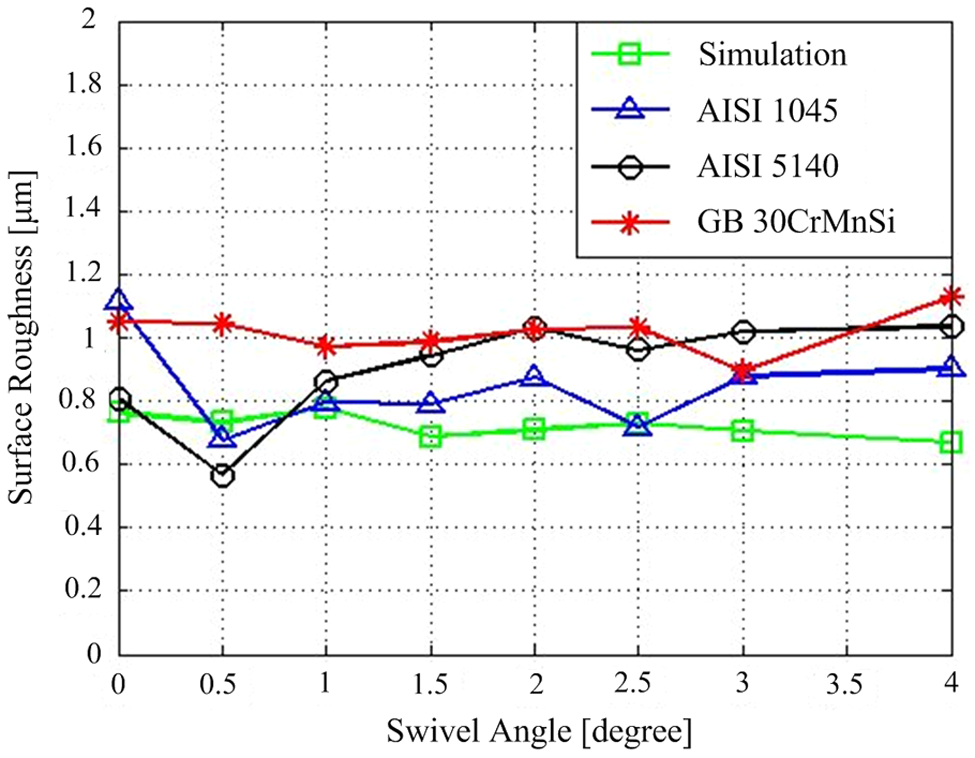
Relationship between surface roughness and swivel angle.
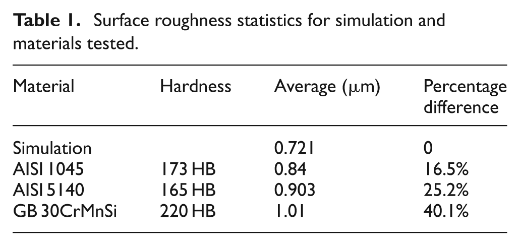
Table 1 summarizes the average workpiece surface roughness Ra and the percentage differences between the numerical simulation and the experimental results. As can be seen in the table, the predicted roughness values are less than the experimentally measured values. The table also shows that the material type did have an effect on surface finish. These differences are believed to be owing to a combination of the following: the model does not include any of the physics associated with metal cutting, such as the ridges created when an abrasive grit pushes its way through the workpiece material. Also, the model does not include any of the machine dynamics, such as chatter that would tend to create a rougher surface finish, especially for harder and tougher materials.
Surface roughness statistics for simulation and materials tested.
The simulator was then used to predict the surface roughness for swivel angles up to 30 degrees and the results are shown in Figure 15. Again, for the grinding conditions simulated, no significant relationship between surface roughness and swivel angle is predicted.
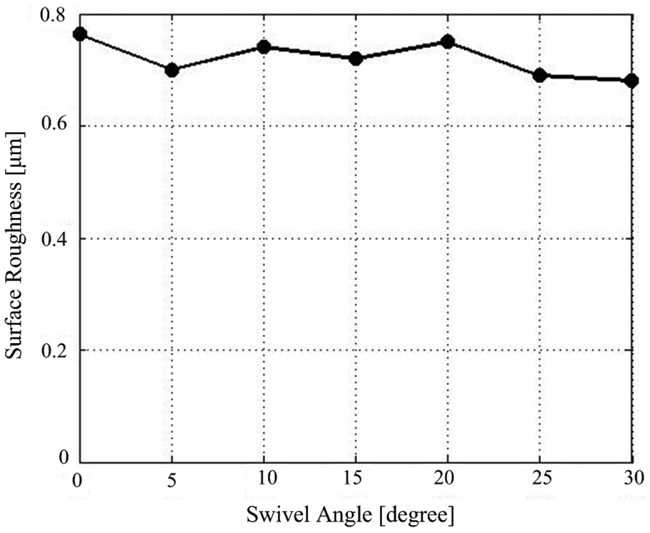
Predicted surface roughness for large swivel angles.
Conclusion
In this article, a numerical approach is proposed to predict 3D workpiece surface topologies for the cylindrical point grinding process. Point grinding experiments were carried out to validate the computer simulator and good agreement was observed for different cutting speeds and swivel angles with an average difference between measured and predicted roughness values Ra of 6.3% for the three cutting speeds tested. It was observed that, for the grinding conditions tested, the swivel angle does not significantly influence the resulting workpiece surface roughness. This important result suggests that one can point grind with different swivel angles to greatly improve the flexibility of the grinding operation without any significant decrease in the quality of the resulting workpiece surface.
Footnotes
Appendix
Funding
The authors would like to thank the National Natural Foundation of China [Grant No. 50775032], the China Scholarship Council (CSC), and the Natural Science and Engineering Research Council of Canada (NSERC) for providing financial support for this research.