Sage Journals: Discover world-class research

Abstract

In this study, the effects of the abrasive waterjet operating variables on the kerf angle were studied and the material properties were correlated with the kerf angle. The Taguchi method was followed to conduct the experimentation and the regression modeling was used in order to build models for prediction of dependent (kerf angle) from independent (operating and material properties) variables. Additionally, the adequacy of the model was tested using several statistical tests. The results indicated that not only operating variables themselves, but also the textural and mineralogical properties had discernible effects on the kerf angles. It was found from the correlation analysis that the water absorption, max grain size of rock-forming minerals and mean grain size of the rock had significant influences on the kerf angles of the rocks tested. Furthermore, it was determined that the kerf angles can be predicted by the developed models related to the rock types.

Keywords

Abrasive waterjet rock kerf angle statistical analysis

Introduction

Abrasive waterjet (AWJ) machining is one of the developing non-traditional manufacturing technologies. It uses a fine jet of ultra-high-pressure water and abrasive slurry to cut material by means of erosion.¹ The technology has found extensive applications in various industries. It has been particularly gaining favor with difficult-to-cut materials, such as ceramics and rocks.² AWJ machining has many distinct advantages over other cutting technologies. However, this machining technology also has some limitations and drawbacks in terms of its cutting capacity; it may generate loud noise and a messy working environment, or create tapered edges on the kerf.³

As in the case of every machining process, the cutting performance of an AWJ is influenced by both operating variables and materials properties. Among these parameters, the operating variables can be controlled during the cutting process; however, the materials properties, owing to the complexity in nature, may not be controlled. The cutting performance is generally evaluated on the basis of attainable depth of cut, kerf width, kerf angle, surface roughness, surface waviness and material removal rate. As an important cutting performance indicator, the kerf angle is a quantity that is often used to reflect the inclination of the kerf wall from the top surface to the bottom of the kerf. It is a special and undesirable geometrical feature inherent to AWJ machining.⁴ In published literature, a wide range of studies for understanding and improving an AWJ, from the standpoint of cutting performance, including the kerf angle has been done so far. However, limited studies investigating the cutting performance of an AWJ in rock cutting have been conducted.^5–9 Additionally, almost no attempt has been found in the relevant literature to model the cutting performance of an AWJ from both operating variables and materials properties to predict the cutting performance of an AWJ in rock cutting. Therefore; this study was aimed at investigating the influence of operating variables on the kerf angles of granitic rocks. Moreover, a correlation technique was employed for determining the significant materials properties on the kerf angles. To model the cutting performance of an AWJ in rock for prediction of kerf angle from both operating variables and materials properties, regression analysis was employed. Additionally, the models derived from the multiple regression analysis were validated through determination coefficients, t-test, F-test, the plots of observed and predicted kerf angles, and residual analysis.

Experimental study

Material

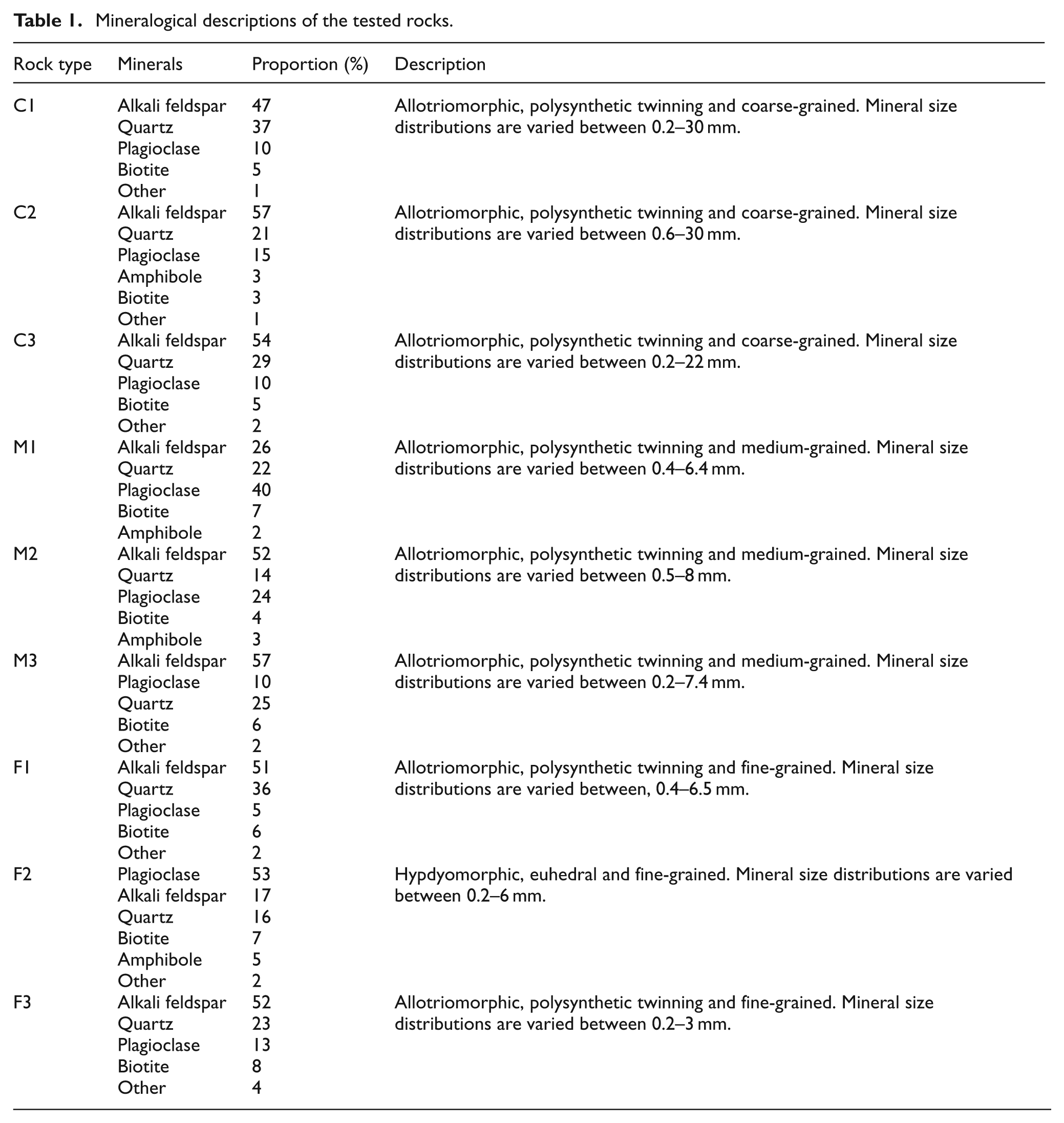
In this study, pre-dimensioned granitic rocks were used as the target material. These materials were provided in a thickness of 3 cm, length of 20 cm and width of 10 cm. The selected rocks include Carmen Red (C1), Baltic Brown (C2), Rosa Minho (C3), Aksaray Yaylak (M1), Giresun Vizon (M2), Azul Platino (M3), Multicolor Red (F1), Bergama Grey (F2) and Balaban Green (F3). (C: coarse-grained; M: medium-grained; F: fine-grained.) Thin sections of the samples were examined under a petrographic microscope for determining the mineral type and content. The point-count method was employed for the modal analyses. These examinations mainly included the determination of modal compositions and grain-size distributions of the rock samples. The mineralogical compositions of the rocks are given in Table 1, along with their textural and granular description. As can be seen from Table 1, quartz, K-feldspar, plagioclase and biotite were the main rock-forming minerals in all samples, varying in their percentage contents. Additionally, grain size distribution of the rock-forming minerals was also determined using a digital image processing software of DeWinter Material Plus 4.1 and the mean grain size of the rock was then calculated.

Table 1.

Mineralogical descriptions of the tested rocks.

Rock type	Minerals	Proportion (%)	Description
C1	Alkali feldspar	47	Allotriomorphic, polysynthetic twinning and coarse-grained. Mineral size distributions are varied between 0.2–30 mm.
	Quartz	37
	Plagioclase	10
	Biotite	5
	Other	1
C2	Alkali feldspar	57	Allotriomorphic, polysynthetic twinning and coarse-grained. Mineral size distributions are varied between 0.6–30 mm.
	Quartz	21
	Plagioclase	15
	Amphibole	3
	Biotite	3
	Other	1
C3	Alkali feldspar	54	Allotriomorphic, polysynthetic twinning and coarse-grained. Mineral size distributions are varied between 0.2–22 mm.
	Quartz	29
	Plagioclase	10
	Biotite	5
	Other	2
M1	Alkali feldspar	26	Allotriomorphic, polysynthetic twinning and medium-grained. Mineral size distributions are varied between 0.4–6.4 mm.
	Quartz	22
	Plagioclase	40
	Biotite	7
	Amphibole	2
M2	Alkali feldspar	52	Allotriomorphic, polysynthetic twinning and medium-grained. Mineral size distributions are varied between 0.5–8 mm.
	Quartz	14
	Plagioclase	24
	Biotite	4
	Amphibole	3
M3	Alkali feldspar	57	Allotriomorphic, polysynthetic twinning and medium-grained. Mineral size distributions are varied between 0.2–7.4 mm.
	Plagioclase	10
	Quartz	25
	Biotite	6
	Other	2
F1	Alkali feldspar	51	Allotriomorphic, polysynthetic twinning and fine-grained. Mineral size distributions are varied between, 0.4–6.5 mm.
	Quartz	36
	Plagioclase	5
	Biotite	6
	Other	2
F2	Plagioclase	53	Hypdyomorphic, euhedral and fine-grained. Mineral size distributions are varied between 0.2–6 mm.
	Alkali feldspar	17
	Quartz	16
	Biotite	7
	Amphibole	5
	Other	2
F3	Alkali feldspar	52	Allotriomorphic, polysynthetic twinning and fine-grained. Mineral size distributions are varied between 0.2–3 mm.
	Quartz	23
	Plagioclase	13
	Biotite	8
	Other	4

Physico-mechanical properties

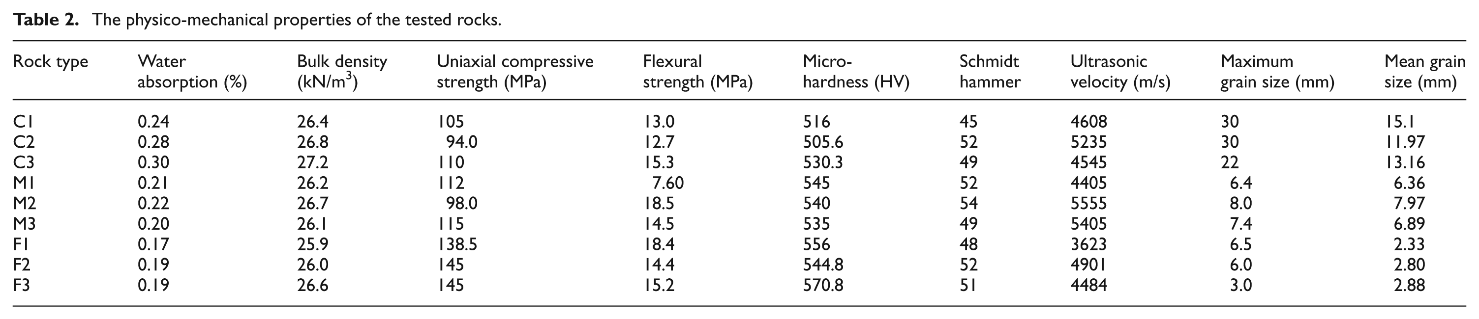
Some physico-mechanical properties of the selected rocks are presented in Table 2. Uniaxial compressive strength (MPa), flexural strength (MPa), bulk density (kN/m³), water absorption by volume (%), ultrasonic velocity (m/s), Schmidt hammer hardness and microhardness (HV) were determined. The process for the laboratory tests were summarized below.

Table 2.

The physico-mechanical properties of the tested rocks.

Rock type	Water absorption (%)	Bulk density (kN/m³)	Uniaxial compressive strength (MPa)	Flexural strength (MPa)	Micro-hardness (HV)	Schmidt hammer	Ultrasonic velocity (m/s)	Maximum grain size (mm)	Mean grain size (mm)
C1	0.24	26.4	105	13.0	516	45	4608	30	15.1
C2	0.28	26.8	94.0	12.7	505.6	52	5235	30	11.97
C3	0.30	27.2	110	15.3	530.3	49	4545	22	13.16
M1	0.21	26.2	112	7.60	545	52	4405	6.4	6.36
M2	0.22	26.7	98.0	18.5	540	54	5555	8.0	7.97
M3	0.20	26.1	115	14.5	535	49	5405	7.4	6.89
F1	0.17	25.9	138.5	18.4	556	48	3623	6.5	2.33
F2	0.19	26.0	145	14.4	544.8	52	4901	6.0	2.80
F3	0.19	26.6	145	15.2	570.8	51	4484	3.0	2.88

Uniaxial compressive and flexural strength

It may be important to note that, in practice, there are serious difficulties of preparing and testing hard rocks, including granites, for their mechanical properties, such as uniaxial compressive and flexural strength. For these reasons, the uniaxial compressive and flexural strengths of the selected rocks were provided by the stone processing company, who supplied the selected rocks.

Bulk density

To determine the bulk density, the ISRM¹⁰ suggested method was used. Bulk volume of samples were calculated with the Archimedes principle. The weight of the sample was determined by a balance, capable of weighing to an accuracy of 0.01 g or percentage of the sample weight. An electronic precision balance was used to weigh samples’ weight and a drying oven was used to dry samples. The bulk density test was applied on ten samples prepared for each rock.¹¹

Water absorption

The test samples were first submitted to vacuum (about 0.7 mbar) for 3 h. After this period, the test samples were saturated in distilled water and submitted again to vacuum during another period of 3 h. The detailed experimental procedure can be also found in the relevant literature.

Ultrasonic velocity

Puntid Plus model ultrasonic testing equipment was used for measuring ultrasonic velocity. Piezoelectric transducers with a natural resonance frequency of 150 kHz were used in the measurements. The ultrasonic pulse velocity was obtained by direct transmission. The connection of the transducers to the sample was improved through the application of an appropriate coupling paste. The transit time was recorded for each sample as the average of ten independent readings. The mean values of the ultrasonic pulse velocity were obtained by dividing the path length by the average transit time of the ten measurements, as suggested by Vasconcelos et al.¹²

Schmidt hammer hardness

ISRM (1981) suggested that 20 rebound values from single impacts, separated by at least a plunger diameter, should be recorded and averaged for the upper ten values. The test method was carried out on all samples. All measurements were carried out in the direction perpendicular to the horizontal surface with an N-type Schmidt hammer.

Microhardness

The microhardness of the samples was measured using a Vickers microhardness meter is an average of 3–5 points for a mineral. It is difficult to identify indention diagonal of various hard brittle minerals owing to the fracture around the indention.¹³ Therefore, a measure load of 100 g was chosen for determining the microhardness. Microhardness stands for a weighed average value of granite microhardness in a whole, concerning mineral microhardness and its weight in granite.

Experimental design

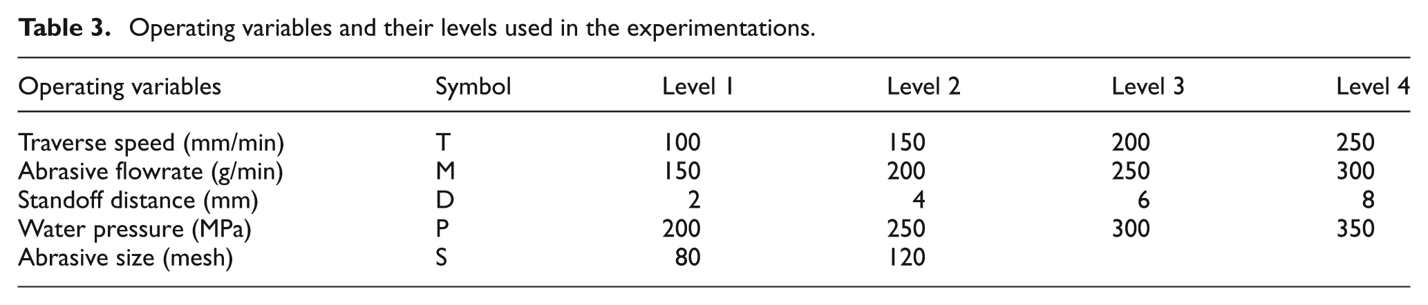
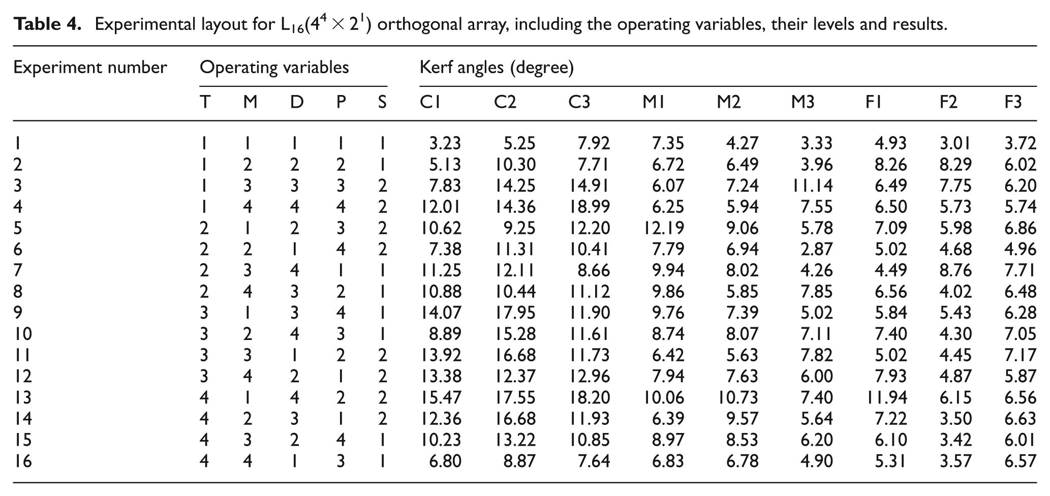
In the study, the operating variables, traverse speed, abrasive flowrate, standoff distance and water pressure were designed by four levels, and abrasive size was designed by two levels (owing to the difficulties for commercially supplying) (Table 3). Those levels were selected based on previous works reported in literature on rock/rocklike cutting by an AWJ.^6,8,14,15 All other machining parameters were kept constant during the experiments. Based on the operating variables and their levels, a standard orthogonal array of L₁₆(4⁴ × 2¹) was found to be appropriate for the experimental layout. In total, 144 runs for nine granites were undertaken in this experimental investigation. Table 4 presents the experimental layout, including the results.

Table 3.

Operating variables and their levels used in the experimentations.

Operating variables	Symbol	Level 1	Level 2	Level 3	Level 4
Traverse speed (mm/min)	T	100	150	200	250
Abrasive flowrate (g/min)	M	150	200	250	300
Standoff distance (mm)	D	2	4	6	8
Water pressure (MPa)	P	200	250	300	350
Abrasive size (mesh)	S	80	120

Table 4.

Experimental layout for L₁₆(4⁴ × 2¹) orthogonal array, including the operating variables, their levels and results.

Experiment number	Operating variables					Kerf angles (degree)
	T	M	D	P	S	C1	C2	C3	M1	M2	M3	F1	F2	F3
1	1	1	1	1	1	3.23	5.25	7.92	7.35	4.27	3.33	4.93	3.01	3.72
2	1	2	2	2	1	5.13	10.30	7.71	6.72	6.49	3.96	8.26	8.29	6.02
3	1	3	3	3	2	7.83	14.25	14.91	6.07	7.24	11.14	6.49	7.75	6.20
4	1	4	4	4	2	12.01	14.36	18.99	6.25	5.94	7.55	6.50	5.73	5.74
5	2	1	2	3	2	10.62	9.25	12.20	12.19	9.06	5.78	7.09	5.98	6.86
6	2	2	1	4	2	7.38	11.31	10.41	7.79	6.94	2.87	5.02	4.68	4.96
7	2	3	4	1	1	11.25	12.11	8.66	9.94	8.02	4.26	4.49	8.76	7.71
8	2	4	3	2	1	10.88	10.44	11.12	9.86	5.85	7.85	6.56	4.02	6.48
9	3	1	3	4	1	14.07	17.95	11.90	9.76	7.39	5.02	5.84	5.43	6.28
10	3	2	4	3	1	8.89	15.28	11.61	8.74	8.07	7.11	7.40	4.30	7.05
11	3	3	1	2	2	13.92	16.68	11.73	6.42	5.63	7.82	5.02	4.45	7.17
12	3	4	2	1	2	13.38	12.37	12.96	7.94	7.63	6.00	7.93	4.87	5.87
13	4	1	4	2	2	15.47	17.55	18.20	10.06	10.73	7.40	11.94	6.15	6.56
14	4	2	3	1	2	12.36	16.68	11.93	6.39	9.57	5.64	7.22	3.50	6.63
15	4	3	2	4	1	10.23	13.22	10.85	8.97	8.53	6.20	6.10	3.42	6.01
16	4	4	1	3	1	6.80	8.87	7.64	6.83	6.78	4.90	5.31	3.57	6.57

Experimental set-up and procedure

The experiments were conducted on an AWJ cutter, consisting of a high output pump with an operating pressure of up to 380 MPa, as schematically shown in Figure 1 [adopted from Duflou et al.¹⁶]. The nozzle diameter and length is 1.1 mm and 75 mm, respectively. The abrasives were delivered using compressed air from a hopper to the mixing chamber and were regulated using a metering disc. The debris of material and the slurry were collected into a catcher tank. On the other hand, garnet chemically consisting of 36% FeO, 33% SiO₂, 20% Al₂O₃, 4% MgO, 3% TiO₂, 2% CaO and 2% MnO₂ was used as an abrasive material for cutting processes. The granites were subjected to cut through their widths. Owing to the variability and accuracy of the experimental data, each granite was cut four times in the same conditions and the cutting performance of the AWJ was evaluated in terms of the kerf angle. Kerf angle is a quantity that is often used to reflect the inclination of the kerf wall from the top surface to the bottom of the kerf. It is a special and undesirable geometrical feature inherent to AWJ machining.⁴ A schematic diagram of the kerf profile and the kerf angle is shown in Figure 2. Also named the kerf wall inclination, the kerf angle for each cut can be determined from equation (1)¹⁷

Figure 1.

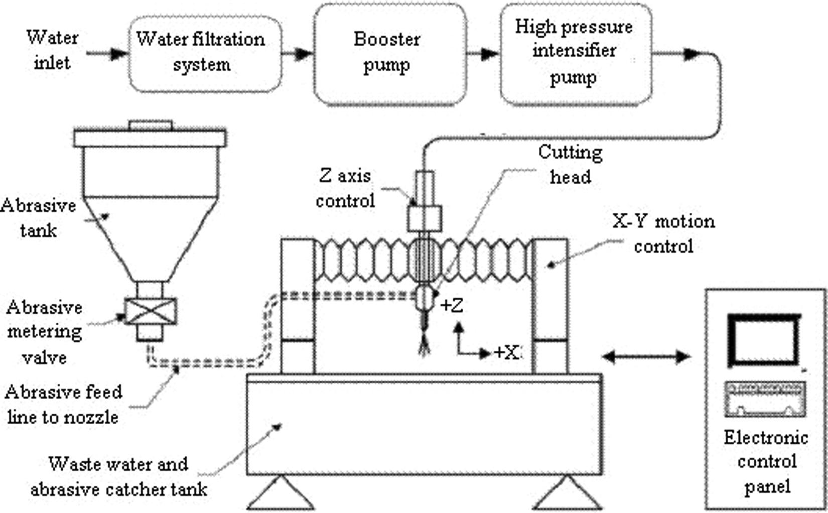
A schematic illustration of the experimental set-up (adopted from Duflou et al.¹⁶).

Figure 2.

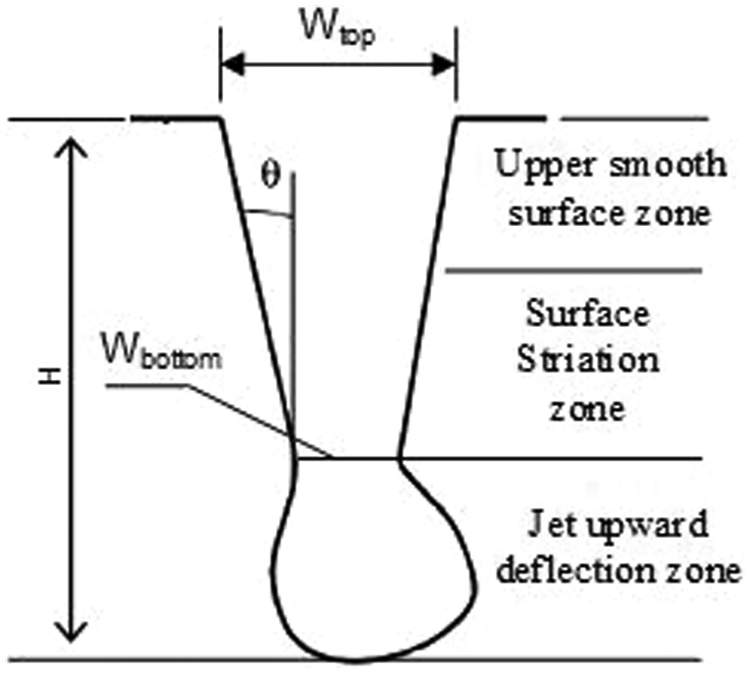
A schematic illustration of the kerf profile and the kerf angle.

θ = \tan^{- 1} (\frac{W_{top} - W_{bottom}}{H})

(1)

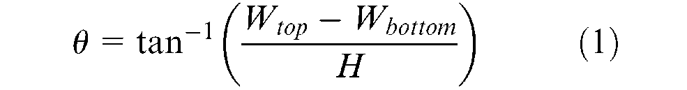
where θ is the kerf angle, W_top and W_bottom are the top and the bottom kerf widths, respectively, and H is the distance from the top of the kerf to where the cut depth is measured. In the present study, following the cutting process, four measurements on each sample for W_top, W_bottom and H were carried out using a vernier caliper, and the average result of these measurements was taken as the final W_top, W_bottom and H for the calculation of kerf angle through the suggested equation.

Results and discussion

The experimental data presented in Table 4 are illustrated in Figure 3, in accordance with the principles of the Taguchi method for presenting the influence of operating variables on the kerf angle. In order to determine the best empirical correlations between independent (material properties) and dependent (kerf angles), a bivariate correlation technique was employed. The multiple regression analysis was then applied to derive the best models for prediction of the kerf angle from both operating variables and material properties. All the statistical analysis was carried out using a statistical software known as “Statistical Package for the Social Sciences (SPSS)”.

Figure 3.

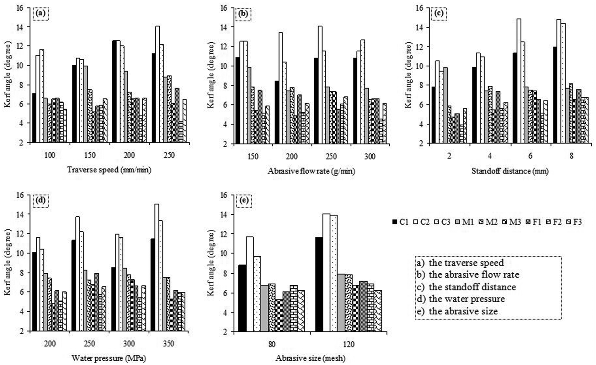
Influence of the operating variables on the kerf angle.

Influence of the operating variables on the kerf angle

Figure 3(a) illustrates the influence of traverse speed on the kerf angle. Within the operating range selected, it can be stated that increasing the traverse speed resulted in an increase in the kerf angle of C1, C2 and C3, despite a decrease reported in the kerf angle of C1 at 250 mm/min, and C2 and C3 at 150 mm/min, respectively. On the other hand, a decrease was initially seen in the kerf angle of F1, and then the kerf angle increased with a further increase in the traverse speed. The kerf angle of the F2 and F3 showed a continuous decrease with traverse speed, although an increase was reported at 100 mm/min for the kerf angle of F3.

The experimental data illustrated in Figure 3(b) shows the influence of the abrasive flowrate on the kerf angle. As seen, increasing the abrasive flowrate resulted in a decrease in the kerf angle of C1, M1 and M2. The kerf angles of C2, F2 and F3 increased with the increasing abrasive flowrate despite a decrease obtained at 300 g/min. Further, the kerf angles of C3, M3 and F1 showed an unsteady trend with the abrasive flowrate.

The experimental results revealed that the kerf angles of for C1, C2, M2 and F3 increased with the increasing standoff distance, as seen in Figure 3(c). Despite a decrease reported at 6 mm for the kerf angles of F1 and F2, and at 8 mm for M3, it can also be pointed out that the kerf angles of M3, F1 and F2 increased with the increasing standoff distance. Among the samples, the kerf angle of M1 showed an unsteady trend with the standoff distance.

The influence of the water pressure on the kerf angles of rocks was depicted in Figure 3(d). It can be concluded that the increasing water pressure resulted in an increase in the kerf angles of C1, C2, C3 and F2, despite a decrease observed at 300 MPa. A similar trend was seen in the kerf angle of M1, M3 and F3. Although the kerf angles increased with the increasing water pressure, a decrease occurred at 350 MPa for M1, M3 and F3. Further, the kerf angle of M2 exhibited an unsteady trend with the increasing water pressure.

In case of the abrasive size, it can be noted that the wider kerf angles were obtained by fine-grained abrasives in all rocks, as shown in Figure 3(e). When jointly considering the rocks, it can be disclosed that the influence of the abrasive size on the kerf angle of medium- and coarse-grained rocks were clearer than those obtained for the fine-grained rocks.

In AWJ cutting applications, the kerf angles generally increase with the increasing traverse speed, which has a considerable effect on the exposure time for the jet interaction on a given area of material, leading to material erosion by abrasive particles and standoff distance, resulting in jet divergence, as confirmed by relevant literature.^17–19 On the other hand, the relevant literature has also confirmed that the kerf angles decreased with the increasing abrasive flowrate owing to the large number of abrasive particles involved in the cutting process and water pressure affecting the energy required for removing the particles from the material.^20,21 However, most of the studies that have been done so far have been conducted on homogenous materials. In other words, contrary to expectations, different results may be obtained in the cutting of heterogeneous materials, such as granitic rocks, owing to the complex structure. As observed in the current study, in some cases, the kerf angles of the rocks did not provide consistent results with the relevant literature. This phenomenon may be attributed to the heterogeneity of the rocks. Since granitic rocks consist of more than one mineral, their behaviors against cutting depend mainly on the grain size, shape of grains, degree of interlocking, type of contacts and mineralogical composition. The amount of minerals and their grain boundaries located through the cutting line, and/or per unit area, may also affect the behaviors of these rocks. Therefore, it can be concluded that not only operating variables themselves have affected the kerf angles, but also the material properties have discernible effects in these kinds of materials. In addition to the statements mentioned above, there could be other evidence for the phenomenon observed, especially for water pressure and abrasive flowrate. It was pointed out in the existing literature that the increasing water pressure may not always result in a decrease in the kerf angles owing to the effective diameter of the jet, since the effective diameter of the jet decreases when the jet exits from the nozzle.²¹ Although the diverged jet has enough energy for moving towards the bottom kerf, it does not have enough cutting force. Thus, this may lead to wider kerfs at the bottom, leading to higher kerf angles. Furthermore, Shanmugam and Masood²⁰ revealed that the kerf angles were not explicitly influenced by the abrasive flowrate. Hence, the researchers indicated that the influence of the abrasive flowrate on the kerf angle can be omitted.

Statistical analysis

In the present study, multiple regression analysis was first performed to produce models for the prediction of the kerf angles from the operating variables. The kerf angle and operating variables were considered as the dependent and independent variables, respectively. The best regression models are given below for the rock types. From the equations presented below, it was seen that the dependent variable kerf angle is seen as a linear function of more than one independent variable. It can also be noted that, apart from the water pressure, all other operating variables were involved in the equations. The dependent and independent variables involved in the models below, denoted by Y_C1, _C2, _C3, _M1, _M2, _M3, _F1, _F2, and _F3, are the kerf angles of the rock types, T (the traverse speed), M (the abrasive flow rate), D (the standoff distance), and S (the abrasive size)

Y c_{1} = - 5.489 + 0.030 T + 0.683 D + 0.070 S

(2)

Y_{C 2} = 3.889 + 0.028 T + 0.821 D

(3)

Y_{C 3} = - 2.892 + 0.817 D + 0.106 S

(4)

Y_{M 1} = 11.446 - 0.0118 M + 0.200 D - 0.016 S

(5)

Y_{M 2} = 2.811 + 0.017 T + 0.322 D

(6)

Y_{M 3} = - 2.15 + 0.012 M + 0.374 D + 0.036 S

(7)

Y_{F 1} = 4.185 - 0.008 M + 0.336 D + 0.026 S

(8)

Y_{F 2} = 5.429 - 0.014 T + 0.323 D + 0.008 S

(9)

Y_{F 3} = 3.52 + 0.006 T + 0.003 M + 0.184 D

(10)

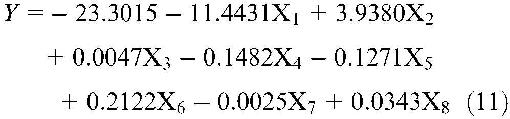
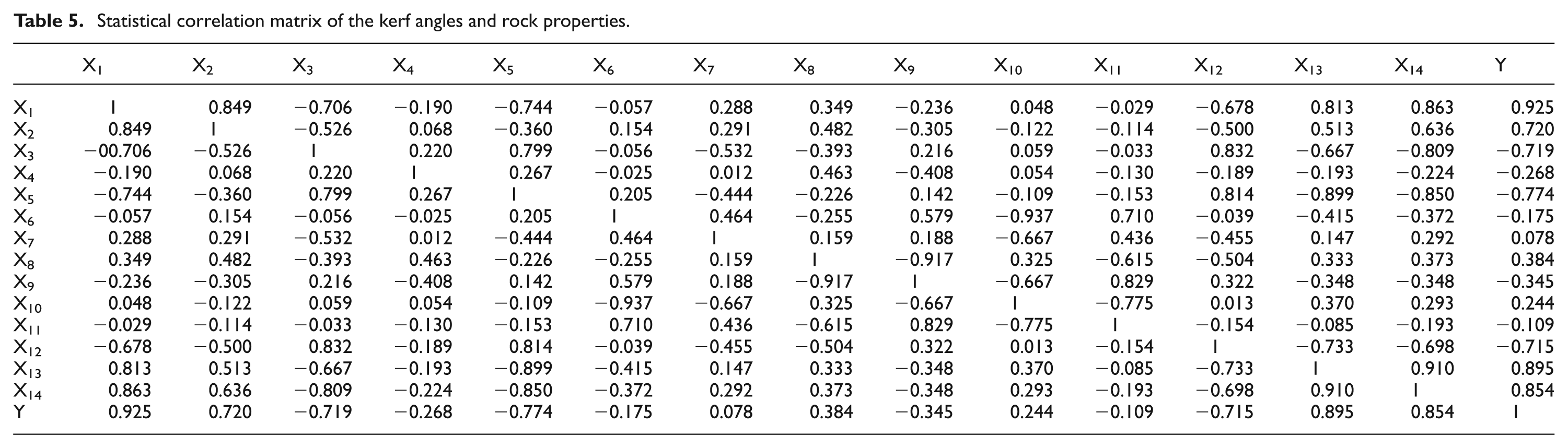
The multiple regression analysis was also performed using the rock properties; water absorption (X₁, %), bulk density (X₂, kN/m³), uniaxial compressive strength (X₃, MPa), flexural strength (X₄, MPa), microhardness (X₅, HV), Schmidt hammer hardness (X₆), ultrasonic velocity (X₇, m/s), alkali feldspar content (X₈, %), plagioclase content (X₉, %), quartz content (X₁₀, %), amphibole content (X₁₁, %), biotite (X₁₂, %), maximum grain size of rock-forming minerals (X₁₃, mm) and mean grain size of the rock (X₁₄, mm). The constant operating variables were chosen to enable a direct comparison of results obtained for all rock samples. Therefore, regression analysis was performed for the experimental data obtained from the first test, where, relatively, the smallest kerf angles were obtained. In this regard, a correlation matrix was initially produced to investigate the strength of the linear relationships between the rock properties and kerf angles of the tested rocks. The models were then developed from backward multiple linear regression analysis for prediction of the kerf angles from the rock properties. In the correlation matrix, a bivariate correlation technique was applied to the original dataset in an attempt to define the degree of linear relationships between all variables. According to the bivariate correlation analysis, presented in Table 5, it can be disclosed that the water absorption (%), maximum grain size of rock-forming minerals (mm) and mean grain size of the rock (mm) have significant correlations on the kerf angles. Additionally, it can be stated that the bulk density (kN/m³), uniaxial compressive strength (MPa), microhardness (HV) and biotite (%) have positive correlations with the kerf angles, while the others have poor correlations. As a result of regression analysis applied for the rock properties, it was determined that the kerf angles can be predicted from eight independent variables, including water absorption (%), bulk density (kN/m³), uniaxial compressive strength (MPa), flexural strength (MPa), microhardness (HV), Schmidt hammer hardness, ultrasonic velocity (m/s) and alkali feldspar content (%). The related regression analysis is

Table 5.

Statistical correlation matrix of the kerf angles and rock properties.

	X₁	X₂	X₃	X₄	X₅	X₆	X₇	X₈	X₉	X₁₀	X₁₁	X₁₂	X₁₃	X₁₄	Y
X₁	1	0.849	−0.706	−0.190	−0.744	−0.057	0.288	0.349	−0.236	0.048	−0.029	−0.678	0.813	0.863	0.925
X₂	0.849	1	−0.526	0.068	−0.360	0.154	0.291	0.482	−0.305	−0.122	−0.114	−0.500	0.513	0.636	0.720
X₃	−00.706	−0.526	1	0.220	0.799	−0.056	−0.532	−0.393	0.216	0.059	−0.033	0.832	−0.667	−0.809	−0.719
X₄	−0.190	0.068	0.220	1	0.267	−0.025	0.012	0.463	−0.408	0.054	−0.130	−0.189	−0.193	−0.224	−0.268
X₅	−0.744	−0.360	0.799	0.267	1	0.205	−0.444	−0.226	0.142	−0.109	−0.153	0.814	−0.899	−0.850	−0.774
X₆	−0.057	0.154	−0.056	−0.025	0.205	1	0.464	−0.255	0.579	−0.937	0.710	−0.039	−0.415	−0.372	−0.175
X₇	0.288	0.291	−0.532	0.012	−0.444	0.464	1	0.159	0.188	−0.667	0.436	−0.455	0.147	0.292	0.078
X₈	0.349	0.482	−0.393	0.463	−0.226	−0.255	0.159	1	−0.917	0.325	−0.615	−0.504	0.333	0.373	0.384
X₉	−0.236	−0.305	0.216	−0.408	0.142	0.579	0.188	−0.917	1	−0.667	0.829	0.322	−0.348	−0.348	−0.345
X₁₀	0.048	−0.122	0.059	0.054	−0.109	−0.937	−0.667	0.325	−0.667	1	−0.775	0.013	0.370	0.293	0.244
X₁₁	−0.029	−0.114	−0.033	−0.130	−0.153	0.710	0.436	−0.615	0.829	−0.775	1	−0.154	−0.085	−0.193	−0.109
X₁₂	−0.678	−0.500	0.832	−0.189	0.814	−0.039	−0.455	−0.504	0.322	0.013	−0.154	1	−0.733	−0.698	−0.715
X₁₃	0.813	0.513	−0.667	−0.193	−0.899	−0.415	0.147	0.333	−0.348	0.370	−0.085	−0.733	1	0.910	0.895
X₁₄	0.863	0.636	−0.809	−0.224	−0.850	−0.372	0.292	0.373	−0.348	0.293	−0.193	−0.698	0.910	1	0.854
Y	0.925	0.720	−0.719	−0.268	−0.774	−0.175	0.078	0.384	−0.345	0.244	−0.109	−0.715	0.895	0.854	1

Y = - 23.3015 - 11.4431 X_{1} + 3.9380 X_{2} + 0.0047 X_{3} - 0.1482 X_{4} - 0.1271 X_{5} + 0.2122 X_{6} - 0.0025 X_{7} + 0.0343 X_{8}

(11)

The determination coefficient of the equation (11) is 1. That means 100% of the variation of the experimental data is explained by the equation. However, the number of the independent variables involved in equation (11) may lead to difficulties for the practical applications. In order to facilitate the applicability of the model, an alternative model for the prediction of kerf angles from the rock properties was also produced. As can be seen, the kerf angles can be predicted by the models developed with less independent variables, including bulk density (kN/m³), microhardness (HV) and ultrasonic velocity (m/s). The determination coefficient of the model presented below, is 0.96. That means, 96% of the variation of the experimental data is explained by

Y = - 22.4409 + 3.6355 X_{2} - 0.1044 X_{5} - 0.0019 X_{7}

(12)

Validation of the models

In the current study; the determination coefficient (R²) of the models, t-test, F-test, plots of observed and predicted kerf widths, and residual analysis were used for verification of the models developed. In the analysis, the F-test and t-test were used to examine the significance of each model and each variable in a model at a 95% significance level, respectively. The models that have an F-ratio larger than the F-ratio from the table (statistical tables) are considered to be significant, and the models that have an F-ratio less than the F-ratio from the table are considered to be insignificant statistically. Similarly, if the variable in a model has a t-value larger than the t-value from the table, the variable is considered to be significant, and if the variable has a t-value less than the t-value from the table, the variable is considered to be insignificant statistically.

The statistical results of the derived models are given in detail in Table 6. The determination coefficients (R²) of the models are above 0.50 for the rock types of C1, C3 and M2, while R² of the models are between 0.40 and 0.50 for rock types C2, M3, F2 and F3. On the other hand, it can be followed from Table 6 that the R² of the models are low for the rock types of M1 and F1 (0.24 and 0.34). These values should normally imply that the variation in the data can be explained by equations (2) to (10) for rock types, since R² provides a measure of how well results are appropriately predicted by the models. Based on the R² values, it can be deduced that the developed models for rock types C1, C3 and M2 present acceptable results, while the developed models for rock types C2, M3, F2 and F3 are within allowable levels. It can be stated that the R² values for the rock types of M1 and F1 failed the test.

Table 6.

Statistical results of the multiple regression models.

Rock type	Independent variables	Coefficient	Standard error	Standard error of estimate	t-value	Tabulated t-value	F-ratio	Tabulated F-ratio	Determination coefficient (R²)
C1	Constant	−5.489	3.670	2.298	−1.495	1.75	7.20	3.28	64.30
	T (mm/min)	0.030	0.010		2.924
	D (mm)	0.683	0.257		2.658
	S (mesh9	0.070	0.029		2.446
C2	Constant	3.889	2.714	2.731	1.432	1.75	6.21	3.28	48.90
	T (mm/min)	0.028	0.012		2.278
	D (mm)	0.821	0.305		2.691
C3	Constant	−2.892	2.464	1.770	−1.173	1.75	20.00	3.28	75.50
	D (mm)	0.817	0.198		4.132
	S (mesh)	0.106	0.022		4.790
M1	Constant	11.446	2.994	1.743	3.823	1.75	1.29	3.28	24.50
	M (g/min)	−0.012	0.008		−1.519
	D (mm)	0.200	0.195		1.030
	S (mesh)	−0.016	0.022		−0.725
M2	Constant	2.811	1.136	1.143	2.473	1.75	8.65	3.28	57.10
	T (mm/min)	0.017	0.005		3.310
	D (mm)	0.322	0.127		2.518
M3	Constant	−2.150	3.071	1.788	−0.700	1.75	2.80	3.28	41.20
	M (g/min)	0.012	0.008		1.509
	D (mm)	0.374	0.199		1.870
	S (mesh)	0.036	0.022		1.617
F1	Constant	4.185	2.820	1.642	1.484	1.75	2.06	3.28	34.00
	M (g/min)	−0.008	0.007		−1.109
	D (mm)	0.336	0.183		1.830
	S (mesh)	0.026	0.020		1.267
F2	Constant	5.429	2.445	1.531	2.219	1.75	2.70	3.28	40.40
	T (mm/min)	−0.014	0.007		−2.103
	D (mm)	0.323	0.171		1.885
	S (mesh)	0.008	0.019		0.377
F3	Constant	3.52	1.139	0.805	3.091	1.75	2.67	3.28	40.00
	T (mm/min)	0.006	0.004		1.754
	M (g/min)	0.003	0.004		0.854
	D (mm)	0.184	0.090		2.048

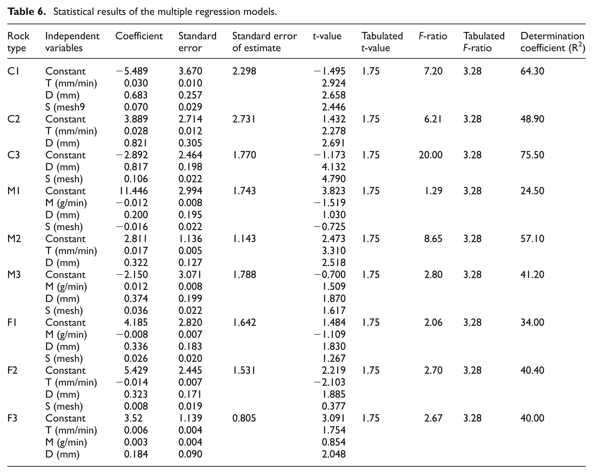
The developed models themselves and variables in the models were validated through the F and t-test. As can be followed from Table 6, the models and their variables for rock types C1, C2, C3 and M2 passed the validation tests of the F and t-test, suggesting that the models and variables are statistically significant. The models and their variables for other rock types, M1, M3, F1, F2 and F3, are statistically insignificant since they failed the validation tests of the F and t-test.

The generality and plausibility of the models were further studied by examining the predicted trends versus the observed trends, as shown in Figures 4 and 5(a). It can be generally concluded from the figures that the predicted and observed results have close values for rock types C1, C2, C3, M2, M3 and F2. As a whole, the results, especially for rock types C1, C2, C3 and M2, indicate that the models can give adequate predictions for the kerf angles for the conditions considered in this study. In other words; these results show that the related models are statistically significant and that the kerf angles may be modeled in this way.

Figure 4.

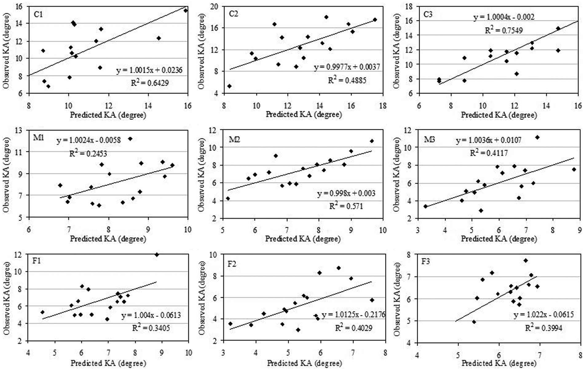
Predicted kerf angles derived from operation variables versus observed kerf angles.

Figure 5.

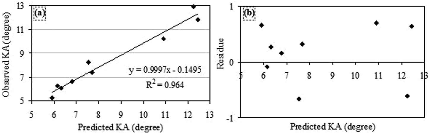
(a) Predicted kerf angles derived from the rock properties versus observed kerf angles. (b) The plots of the residuals against the predicted values.

Another validation method, used for checking the models, is the direct comparison of model and real data in the form of residuals owing to the importance given to clues about the appropriateness of the model. This technique presents a better test providing very effective means of detecting abnormal behavior in the residuals. Therefore, scatter plots were studied to investigate the distribution of residuals (Figures 5(b) and 6). In general, it can be disclosed that the residuals are randomly scattered around the line confirming the correctness of the statistically significant models.

Figure 6.

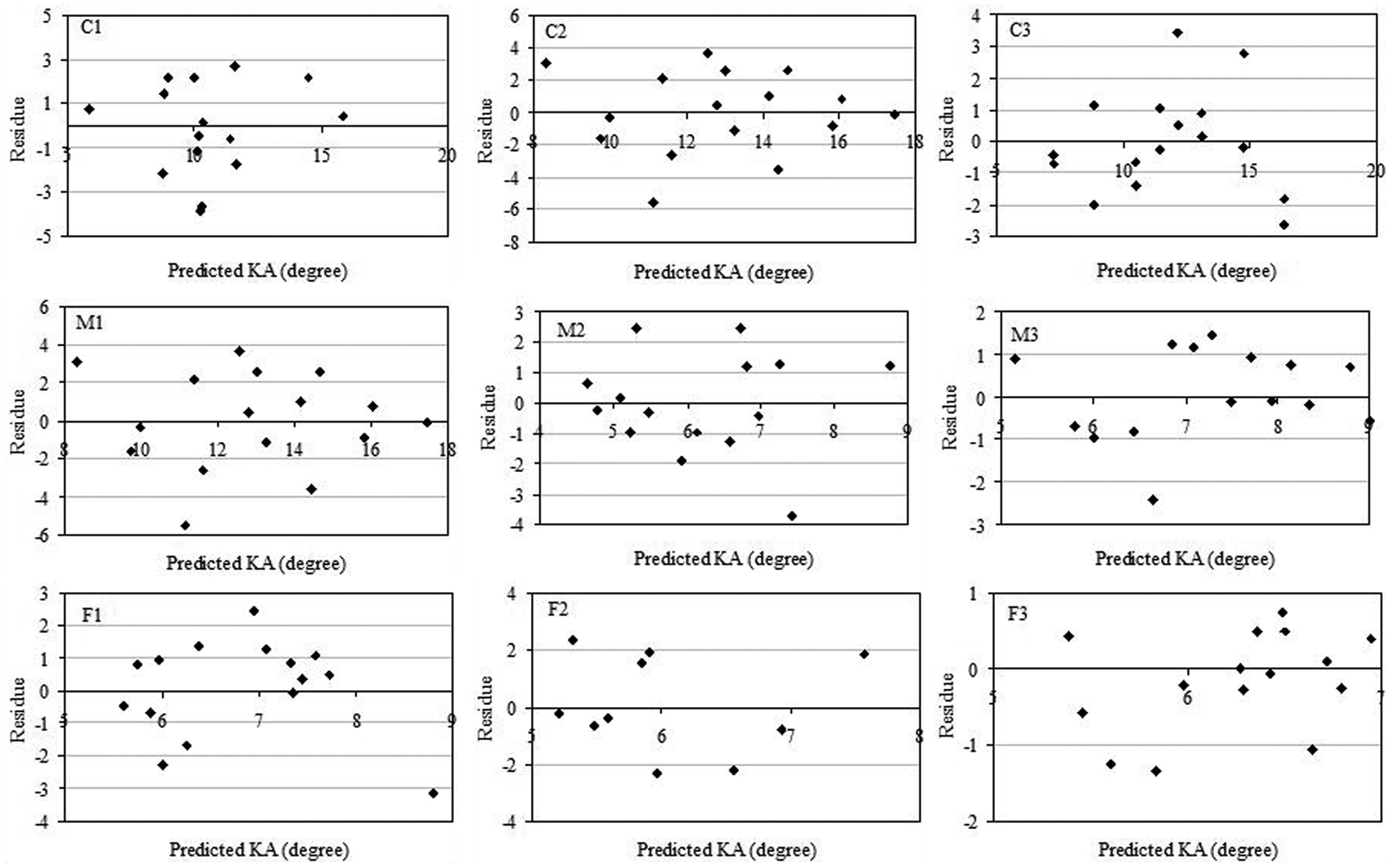
The plots of the residuals against the predicted kerf angles derived from the operating variables.

Conclusions

When jointly considering the influence of the operating variables, it was concluded that, heterogeneity, the rocks resulted in unexpected trends in the kerf angle for some levels of operating variables. Therefore, it can be concluded that, not only operating variables themselves, but also the material properties, have discernible effects in these kinds of materials. Among the material properties, the size and shape of grains, degree of interlocking, type of contacts and mineralogical composition, the amount of minerals and their grain boundaries inside the rocks may have discernible influence on the kerf angles. Additionally, it was found that the water absorption, maximum grain size of rock-forming minerals and mean grain size of the rock have significant correlations on the kerf angles. It was also concluded that the bulk density, uniaxial compressive strength, microhardness and biotite have positive correlations with the kerf angles of the granitic rocks tested. Further, the modeling results and verification methods showed that the derived models relating to the rock types are statistically significant and that the kerf angles may be modeled in this way with respect to the rock types.

Footnotes

Funding

This research received financial support from TÜBİTAK (The Scientific and Technological Research Council of Turkey) [Project No 108M370].

References

Wang

Kuriyagawa

Huang

. An experimental study to enhance the cutting performance in abrasive waterjet machining. Mach Sci Technol 2003; 7(2): 191–207.

Aydin

Karakurt

Aydiner

. An investigation on the surface roughness of the granite machined by abrasive waterjet. B Mater Sci 2011; 34(4): 985–992.

Pon Selvan

Sundara

Rajavel

. Effects of process parameters on depth of cut in abrasive waterjet cutting of cast iron. Int J Sci Eng Res 2011; 2(9): 1–5.

Shanmugam

Wang

Liu

. Minimisation of kerf tapers in abrasive waterjet machining of alumina ceramics using a compensation technique. Int J Machine Tools Mfg 2008; 48: 1527–1534.

Agus

Bortolussi

Ciccu

. The influence of rock properties on waterjet performance. In: Proceedings of 7th American water jet conference, Seattle, Washington, USA, 1993, pp.427–442.

Miranda

Lousa

Miranda

MJA

. Abrasive waterjet cutting of Portuguese Marbles. In: Proceedings of 7th American water jet conference, Seattle, Washington, USA, 1993, pp.443–457.

Magyari

Ilias

Radu

. The influence of rock parameters during the cutting process using high pressure waterjets. In: Proceedings of 10th American water jet conference, Houston, Texas, USA, 1993, pp.479–484.

Hlaváč

Hlaváčová

Gembalová

. Experimental method for the investigation of the abrasive water jet cutting quality. J Mater Process Tech 2009; 209: 6190–6195.

Karakurt

Aydın

Aydıner

. An experimental study on the cut depth of the granite in abrasive waterjet cutting. Mater Mfg Process 2012; 27(5): 538–544.

10.

ISRM. Rock characterization testing and monitoring suggested methods, Brown

(ed). Pergamon Press, 1981, pp.211.

11.

Bilim

. Determination of drillability of some natural stones and their association with rock properties. Sci Res Essays 2011; 6(2): 382–387.

12.

Vasconcelos

Lourenço

Alves

ACS

. Prediction of the mechanical properties of granites by ultrasonic pulse velocity and schmidt hammer hardness. In: North American masonry conference, St. Louis, Missouri, USA, 2007, pp.980–991.

13.

Xie

Tamaki

. Parameterization of micro-hardness distribution in granite related to abrasive machining performance. J Mater Process Tech 2007; 186: 253–258.

14.

Huang

Hou

Wang

. The effect of high pressure abrasive water jet cutting parameters on cutting performance of granite. Key Eng Mater 2006; 304–305: 560–564.

15.

Lauand

Martin

Hennies

. Performance of waterjet cutting system in dimension stone. In: Proceedings of the 11th. American water jet conference, Minneapolis, Minnesota, USA, 2001, pp.427–449.

16.

Duflou

Kruth

Bohez

. Contour cutting of pre-formed parts with abrasive waterjet using 3-axis nozzle control. J Mater Process Tech 2001; 115: 38–43.

17.

Wang

Guo

. The cutting performance in multipass abrasive waterjet machining of industrial ceramics. J Mater Process Tech 2003; 133: 371–377.

18.

Hamatani

Ramulu

. Machinability of high temperature composites by abrasive waterjet. J Eng Mater Tech 1990; 112: 381–386.

19.

Shanmugam

Chen

Siores

. Comparative study of jetting machining technologies over laser machining technology for cutting composite materials. Comp Struct 2002; 57(1–4): 289–296.

20.

Shanmugam

Masood

. An investigation on kerf characteristics in abrasive waterjet cutting of layered composites. J Mater Proces Tech 2009; 209: 3887–3893.

21.

Hocheng

Chang

. Material removal analysis in abrasive waterjet cutting of ceramic plates. J Mater Proces Tech 1994; 40(3–4): 287–304.

A study on the prediction of kerf angle in abrasive waterjet machining of rocks

Abstract

Keywords

Introduction

Experimental study

Material

Physico-mechanical properties

Uniaxial compressive and flexural strength

Bulk density

Water absorption

Ultrasonic velocity

Schmidt hammer hardness

Microhardness

Experimental design

Experimental set-up and procedure

Results and discussion

Influence of the operating variables on the kerf angle

Statistical analysis

Validation of the models

Conclusions

Footnotes

Funding

References