
Abstract
Finite element simulation of metal machining requires accurate constitutive models to characterize the material stress–strain response in plastic deformation processes. An optimization methodology using genetic algorithms was developed to determine the Johnson–Cook material model for Ti–6Al–4V alloy. The optimization of the parameters resulted in lower errors between the calculated flow stress and the experimental values obtained through the split Hopkinson pressure bar tests at different temperatures (ranging from 25 °C to 900 °C) and strain rates (2000 and 2500s−1). Optimized Johnson–Cook constitutive parameters were used to calculate the flow stress under various conditions. The calculated results showed excellent agreement with the experimental values, with errors lower than 4%. In addition, Ti–6Al–4V alloy orthogonal cutting experiments were carried out to validate the finite element simulation results. The experimental chip morphology was compared with the simulation results obtained by the optimized Johnson–Cook model (M2) and the original Johnson–Cook model (M1). The simulated results (including chip morphology and cutting force) were affected by the flow stress model. Comparison of the experimental and simulated results revealed that the optimized Johnson–Cook model can provide relatively good prediction results for the titanium alloy machining process, especially for chip morphology prediction.
Introduction
Titanium alloys have become popular materials in aerospace and medical industries because of their combined properties, such as high stiffness, low density, excellent corrosion and oxidation resistance. 1 Titanium alloys are difficult-to-machine materials because of the high flow stress at elevated temperatures and the sensitivity of these materials to the processing parameters of the forming process. 2 Therefore, understanding the machining mechanics and improving machining efficiency have become increasingly important for the industrial application of titanium alloy. The finite element (FE) method has recently emerged as an essential modeling methodology because of its efficiency and usefulness to decrease the cost of experiments in machining. This method is also a convenient technique to acquire the machining parameters that are difficult to obtain experimentally, such as stress, strain, temperature, etc. Metal cutting always involves large strain (1–10), high strain rate (103–106 s−1) (Jaspers and Dautzenberg 3 ) and a wide range of temperatures. A material constitutive equation plays a key role in characterizing the deformation behavior in machining. Several material models have been developed to determine the deformation behavior under high strain rate conditions. Cockroft and Latham 4 developed the Cockroft–Latham model according to the density of strain energy. Johnson and Cook 5 presented the Johnson–Cook (J–C) model, considering the influence of strain, strain rate and temperature on flow stress. Zerilli and Armstrong 6 developed the Zerilli–Armstrong model based on the dislocation mechanics theory. Recently, Calamaz et al. 1 presented the hyperbolic tangent (TANH) model considering the effect of strain softening. Some of these models are considered as semi-empirical constitutive models that are widely used in existing FE simulation of metal cutting processes. 7 The material parameters of the J–C model, one of the most widely used models, 8 are commonly obtained through split Hopkinson pressure bar (SHPB) tests. This experimental technique is commonly used to assess the deformation behavior at strain rates ranging from 102 s−1 to 104 s−1, 9 so the J–C model parameters obtained by SHPB tests can be applied to simulate machining processes under high strain rate conditions.
Many studies have applied the J–C model in machining simulation. Umbrello et al. 10 used the J–C constitutive equation with different J–C parameters to simulate AISI 316L steel machining and found that the residual stresses are very sensitive to the J–C model parameters. Özel 11 applied the J–C model in a three-dimensional FE model to simulate the AISI 4340 turning process and investigated the influence of the micro-geometry edge on forces, stress and tool wear of polycrystalline cubic boron nitride (PCBN) inserts. Chen et al. 12 presented a ductile failure FE model based on the J–C constitutive model to simulate Ti–6Al–4V alloy high-speed machining.
The material parameters are crucial to the accuracy of the J–C model. The J–C parameters are usually fitted according to the strain–stress curves obtained through SHPB tests. 13 Seo et al. 9 determined the J–C parameters using SHPB tests at 1400 s−1 strain rate and from room temperature to 1000 °C. Lee and Lin 14 fitted J–C model parameters using SHPB tests to study the high-temperature deformation behavior of Ti–6Al–4V alloy under different strain rates. However, the fitting method for the J–C model parameters was not discussed in the article. According to the study of Karpat, 15 the flow stress calculated from the J–C model parameters listed in Lee and Lin 14 do not agree very well with the experimental data at a strain rate of 800 s−1 and at room temperature.
Optimization technologies were developed to determine constitutive model parameters using various objective functions to assess the difference between experimental and computed data. Dusunceli et al. 16 applied the genetic algorithm (GA) optimization technique to determine the parameters for the viscoplasticity model based on overstress (VBO model) by minimizing the errors between experimental and simulated stress. Besides, Cao and Lin 17 developed an optimization technique focused on objective function to determine material constants in creep/viscoplastic constitutive equations based on experimental data. Similarly, Anaraki et al. 18 presented an inverse method to determine the material constants for AZ61 magnesium alloy by minimizing the errors between calculated and experimental results.
Very few studies have focused on the optimization of constitutive model parameters under high strain rate conditions. Lin and Yang 19 applied a GA-based multi-objective optimization technique to determine the viscoplastic constitutive equations for titanium alloy with low strain rates (5 × 10⁻⁵–1 × 10⁻³ s−1) at 927 °C. Recently, Özel and Karpat 20 applied the cooperative particle swarm optimization (CPSO) method to identify the J–C parameters by SHPB tests in Lee and Lin, 21 considering the influence of different temperatures at a strain rate of 2000 s−1. Although optimization techniques are currently widely used to obtain a material constitutive model, very few studies have reported on the application of model optimization results. As the J–C model is commonly applied to characterize the material deformation behavior in machining, it is necessary to use machining simulation to validate the optimized J–C constitutive parameters.
There is a similarity in the deformation behaviors of SHPB tests and machining under high strain rate conditions. Therefore, a GA-based optimization technique is presented in the current study to calculate the J–C parameters according to the SHPB tests under different high strain rates and temperatures. Afterwards, the optimized J–C model parameters are applied in machining simulations to validate the optimization results.
Johnson–Cook model
To model the plastic behavior of Ti–6Al–4V alloy, the J–C constitutive model was employed, which can be represented by the following equation 5
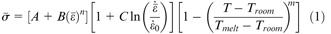
where
Some J–C parameter sets for Ti–6Al–4V alloy are listed in Table 1. Although some of these sets are based on the same SHPB test data, the calculated J–C parameters vary in a wide range owing to the possible differences in microstructures and/or the mathematical techniques applied in calculation. 15 Different material parameters will lead to different simulation results when the J–C model is applied in machining simulation. Umbrello et al. 10 studied the influence of J–C parameters on the results of AISI 316L steel machining simulation. Besides, Umbrello 24 investigated the effect of J–C model parameters on the predicted segmented chip morphology in Ti–6Al–4V alloy orthogonal cutting simulation. These previous studies have demonstrated that material constitutive parameters have a significant impact on simulation results, such as residual stresses, forces and chip morphology. Lee and Lin 14 performed the SHPB tests at different temperatures and strain rates, and they developed a set of J–C parameters according to the test results. However, the stress calculated by the J–C parameters presented in the article did not agree very well with the experimental data, i.e. the stress at 800 s−1 strain rate and at 25 °C (Figure 1). Thus, the main objective of this study is to acquire a set of accurate J–C model parameters using an optimization method according to the experimental results of SHPB tests in Lee and Lin. 14
J–C model parameters for Ti–6Al–4V alloy.
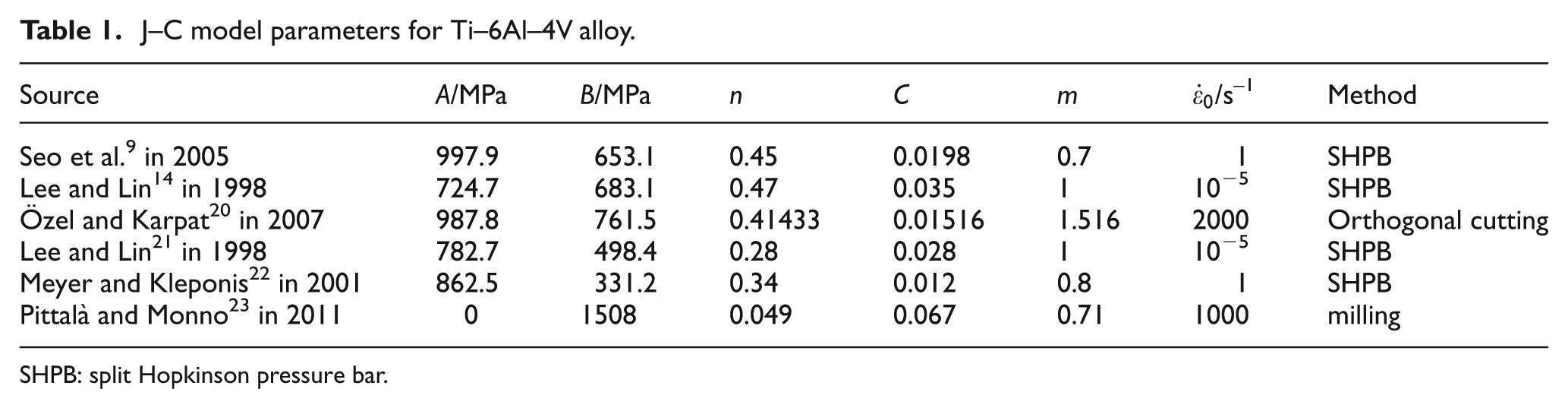
SHPB: split Hopkinson pressure bar.
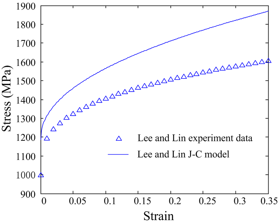
The flow stress calculated by J–C parameters of Lee and Lin 14 and the SHPB test results at 800 s−1 and 25 °C.
Determination of constitutive parameters by genetic algorithm
Objective function
Optimization techniques can be applied to identify material parameters by minimizing a particular norm of the errors between the calculated and the experimental results without any conversion. 25 Two objective functions are defined in the present study in terms of a particular form of difference between the calculated and experimental data for a stress–strain curve.
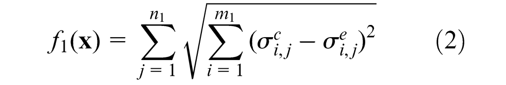
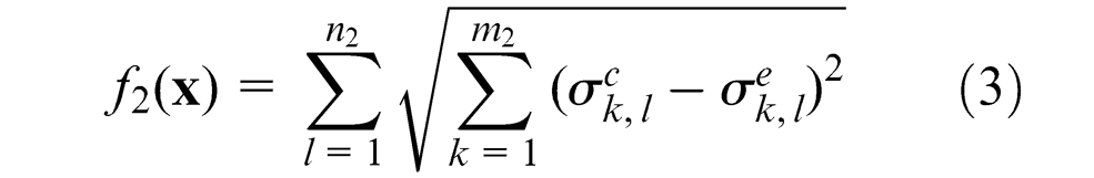
where f1(

to represent the measured stress–strain relationship under each strain rate and temperature condition. Therefore,
The ultimate objective is to acquire a set of appropriate parameters to minimize f1(


where c1 and c2 are weight coefficients for f1(
Computation procedure
Compared with the conventional optimization methods, the GA has the advantage of solving the constrained non-linear optimization problem. This technique is a stochastic search method based on evolution and genetics, exploiting the concept of survival of the fittest.
27
A fitness function F(

where C0 is a predefined constant to ensure that the fitness function has a positive value.
The schematic of the GA optimization procedure is shown in Figure 2. The step-by-step optimization process is outlined as follows.
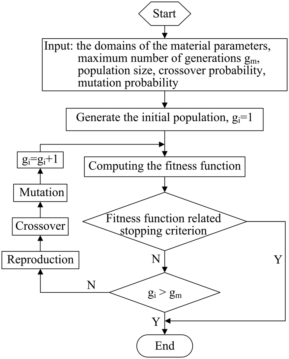
The schematic of GA optimization procedure.
The design variables of the optimization are chosen and the domains of material parameters are inputted. The population size k, maximum number of generation gm, crossover probability λc and mutation probability λm are defined before the optimization program is started.
The initial population is generated randomly.
Each individual
The optimization procedure is terminated if the fitness function related stopping criterion (the weighted average change of the fitness function value is less than function tolerance over a specified generations) is satisfied, i.e. the mean fitness of the population does not evolve after a finite number of generations. Otherwise, if gi > gm, then optimization is terminated.
If the stopping criteria are not satisfied, then the genetic operators, such as reproduction, crossover and mutation on the population are executed (Figure 3). The individuals in population
The children population is generated by reproduction, crossover and mutation operations. The number of generations is set as gi = gi + 1. Step 3 is repeated until one of the termination criteria is satisfied.
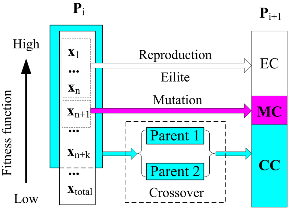
The genetic operators of the GA optimization.
The GA technique can overcome the difficulty of choosing the correct initial values for the constants that exist in traditional optimization techniques. 19 The domains of design variables (J–C parameters) and the variables of optimization are specified at the beginning: the population size k = 1000, maximum number of generation gm = 100, crossover probability λc = 0.8 and mutation probability λm = 0.06. The domains of J–C parameters are defined as 700 MPa ≤ A ≤ 1000 MPa, 600 MPa ≤ B ≤ 1000 MPa, 0 ≤ n ≤ 1, 0 ≤ C ≤ 1 and 0.5 ≤ m ≤ 1.5. The initial population is generated within the domains. The GA procedure begins with the initial population that is composed of random individuals, i.e. the design variables. Then, the optimal design variables are determined by computing the fitness function, generation by generation until one of the termination criteria is reached.
Optimization results
The objective function is calculated using equations (2) to (6) to minimize the difference between the experimental and calculated stresses. The experimental data are obtained by SHPB tests from Lee and Lin. 14 The stress–strain data at different temperatures (25 °C, 300 °C, 500 °C, 700 °C, 900 °C and 1100 °C) are considered in the objective function. The strain rate in machining processes is high and varies with cutting speeds. Therefore, two different strain rates, 2000 and 2500 s−1, are also involved in the objective function. The referenced experimental flow stress curves are shown in Figure 4. Although the flow stress is affected by temperature and strain rate, the effect of temperature is more pronounced than that of strain rate.

Stress–strain responses based on the data of Lee and Lin 14 at different temperatures and strain rates.
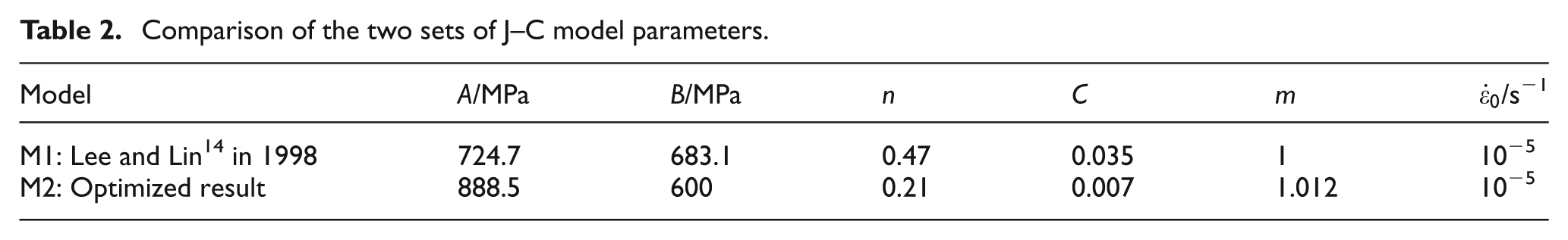
The flow stress of the J–C model is calculated using equation (1). The objective function of the GA-optimized result is shown in Figure 5. The design variables (M2) obtained by the GA optimization and the fitted J–C model (M1) given by Lee and Lin 14 are listed in Table 2.
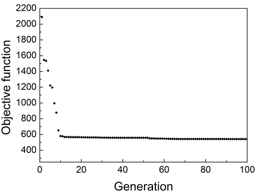
The objective function result of the optimization procedure.
Comparison of the two sets of J–C model parameters.
Using the GA technique, the value of the objective function decreases rapidly within the first ten generations, i.e. the difference between the experimental and calculated flow stress is minimized markedly in the first ten generations compared with subsequent generations. Afterwards, the value of the objective function decreases gradually toward a stable value, until it reaches 542.6 when the optimization is terminated. That is, the specified error (calculated by equations (2) to (5)) between the experimental and calculated stress using the optimized J–C model M2 (Table 2) is 542.6, whereas the error between the experimental and calculated stress using the J–C model M1 (Table 2) is 7836.2. Therefore, the flow stress calculated using J–C model M2 is closer to the experimental flow stress than that calculated using model M1 at the specified temperatures and strain rates as mentioned above.
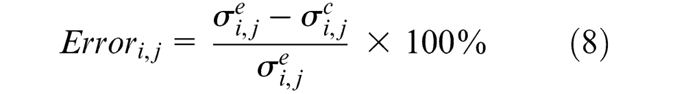
The experimental and calculated flow stress at different temperatures is shown in Figure 6(a) and (b). The calculated values are obtained using the optimized J–C model M2. The errors between experimental and calculated stress (given by equation (8)) at different temperatures are shown in Figure 7(a) and (b). The calculated flow stress shows excellent agreement with the experimental values, except for a few data at the deformation initiation when

Comparison of experimental 14 and calculated flow stress obtained by optimized J–C model M2 at different temperatures: (a) strain rate = 2000 s−1; (b) strain rate = 2500 s−1.

Errors between experimental 14 and calculated flow stress obtained by optimized J–C model M2 at different temperatures: (a) strain rate = 2000 s−1; (b) strain rate = 2500 s−1.
In order to see the optimized results at different strain rates (2000 and 2500 s−1), the flow stress calculated by the J–C model with two sets of parameters (M1 and M2 in Table 2) and the experimental results obtained by the SHPB test at 300 °C and 900 °C are shown in Figure 8(a) and (b). A strain rate hardening phenomenon is evident, both in the experimental and calculated curves. A higher strain rate leads to higher stress at identical temperatures. However, the sensitivity of the strain rate hardening is weak at the two aforementioned strain rates, especially for the calculated results. For instance, the maximum distance of experimental stress at the two different strain rates is 20 MPa, whereas that of calculated stress using M2 is 2 MPa, at a temperature of 900 °C. This phenomenon may be related to the objective function of the GA procedure, which aims to minimize the errors between experimental and calculated stresses at the two different strain rates. On the other hand, the stress calculated by model M2 is closer to the experimental results than that calculated by M1 at temperatures of 300 °C and 900 °C (Figure 8).

Comparison of experimental 14 and calculated flow stress obtained by J–C models M1 and M2 at different strain rates: (a) T = 573 K; (b) T = 1173 K.
Ti–6Al–4V alloy machining simulation for model parameters validation
Ti–6Al–4V alloy orthogonal cutting experiments
A set of FE simulation and titanium alloy orthogonal cutting experiments were developed to evaluate the accuracy of the optimized J–C model parameters in describing material deformation behavior of the machining process. In this work, three different tests (Test1: v = 60 m/min, f = 80 µm/rev; Test2: v = 80 m/min, f = 100 µm/rev; and Test3: v = 130 m/min, f = 100 µm/rev) were performed for a Ti–6Al–4V alloy orthogonal dry cutting experiment and FE simulation.
The orthogonal cutting experiments were performed on a vertical machining center type NEXUS410B-HS. The workpiece was composed of Ti–6Al–4V alloy disks 100 mm in diameter and 2.03 mm thick. The experiment set-up is shown in Figure 9. The cutting tool was an uncoated carbide insert type TPGN 110304 (Kennametal Inc.) with 3° rake angle, 8° clearance angle and 0° inclination angle. The cutting edge radius was approximately 5 μm. The cutting forces were monitored by a dynamometer (Kistler 9257A) and a charge amplifier (Kistler 5070A). A new insert was used for each test to avoid tool wear in the cutting process.
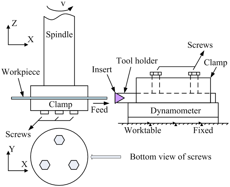
Schematic diagram of the orthogonal cutting experiment set-up.
FE modeling
A two-dimensional (2D) FE model was developed to validate the optimized J–C model parameters by comparing the experimental and simulated results. The geometry of the 2D FE model is shown in Figure 10. The workpiece was meshed with 8000 plane strain thermally coupled quadrilateral elements (type CPE4RT), and the tool was meshed with 255 elements. The characteristic dimensions of the tool were in accordance with the experimental condition: rake angle α = 3°, clearance angle β = 8° and edge radius r = 5 μm. The workpiece was fixed, meanwhile, a velocity along the X direction was exerted on the tool to accomplish the cutting process.
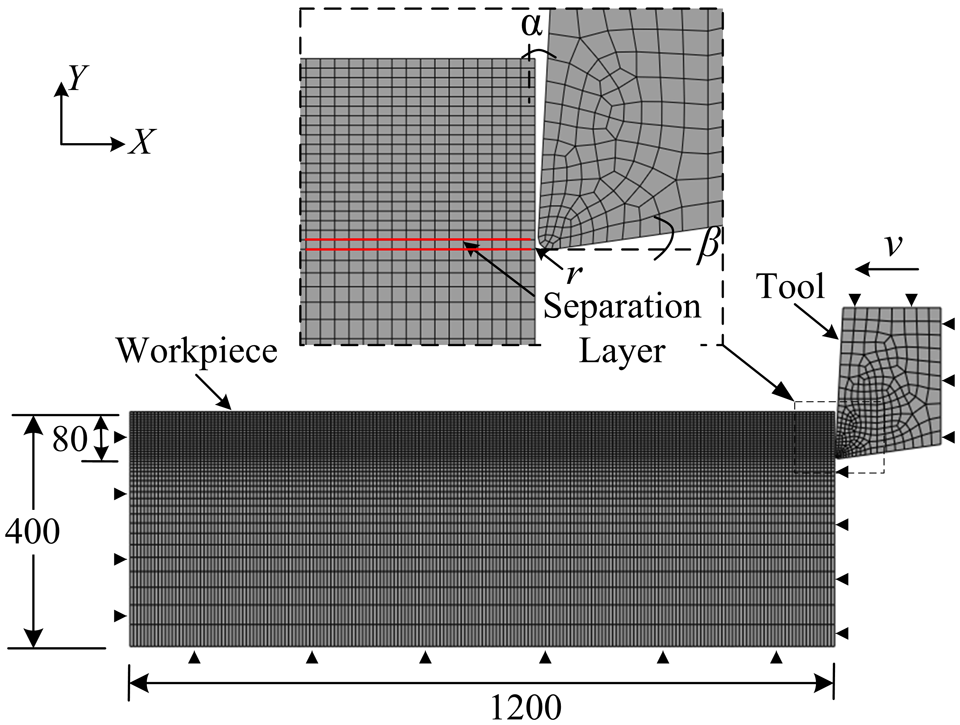
The geometry of the cutting FE model (f = 80 μm/rev).
The J–C plastic material model (equation (1)) and an energy density-based ductile failure criterion, which was illustrated in a previous work, 12 were applied to the FE model in the cutting simulation. Besides the energy density failure criterion, a shear failure criterion is assigned to a separation layer to separate the chip from the workpiece (Figure 10). The failure parameters were identical to those of the previous work. 12
The cutting conditions of the simulation were in accordance with those in the orthogonal cutting experiments. The J–C model M1 and the optimized model M2 (Table 2) were both applied in the cutting simulation to compare the original and optimized J–C model parameters. Except for the changes of J–C model parameters, the other parameters remained unchanged to study the effect of material parameters on the machining simulation.
Simulation results and discussion
The predicted and experimental chip morphology is shown in Figure 11, in which Figure 11(a)–(c) are predicted using model M1, whereas Figure 11(a’)–(c’) are predicted using model M2.
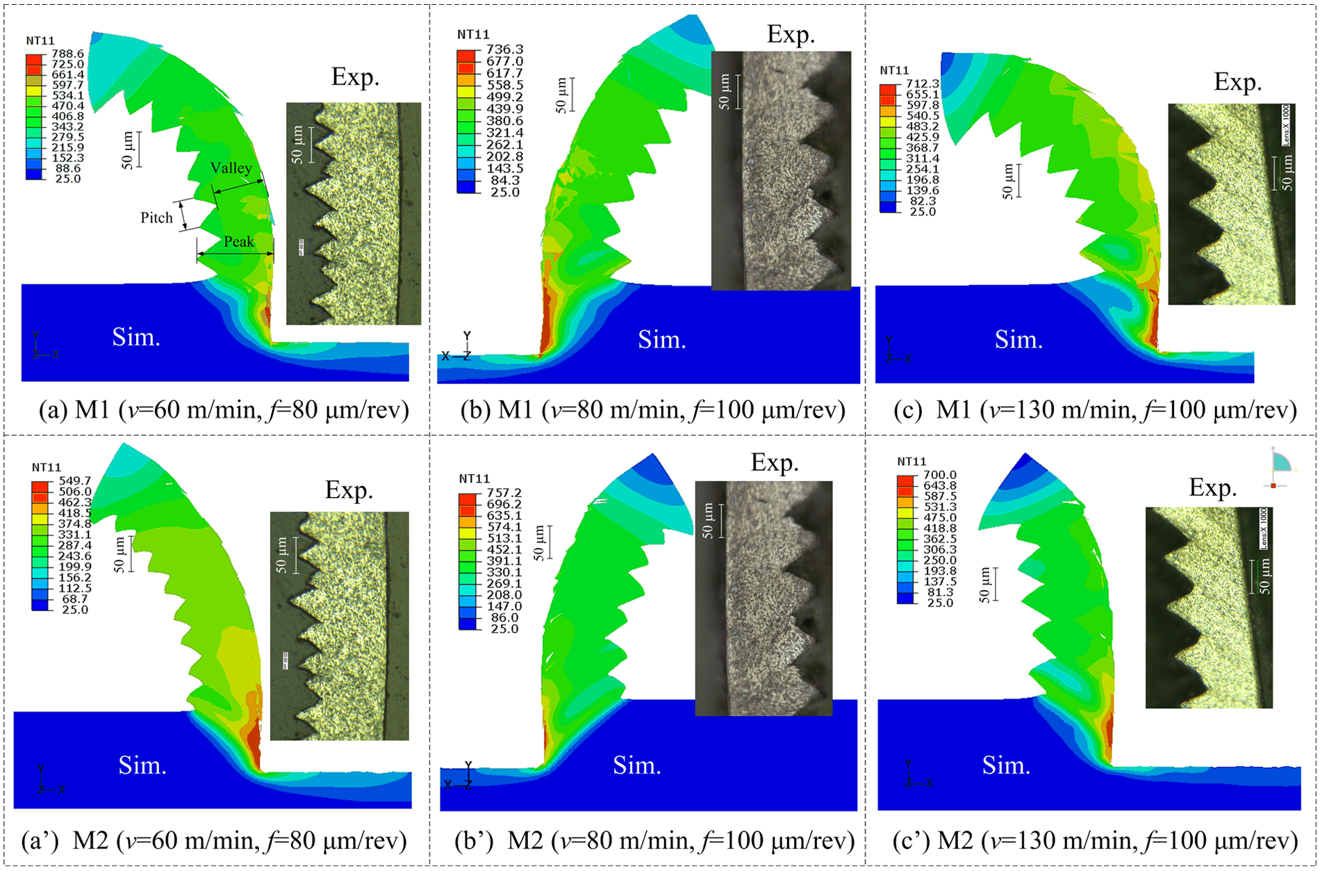
Comparison of experimental chip morphology (Exp.) and simulation results (Sim.) obtained by J–C models M1 and M2 in various cutting conditions.
Obvious segmented chip morphology exists both in the predicted and experimental results. The predicted temperature distribution is illustrated in the simulation results. Many studies have discussed the mechanism of segmented chip formation. Calamaz et al. 1 classified the mechanism of chip formation into two groups: 1) the thermoplastic instability; 2) the crack initiation and propagation. Hua and Shivpuri 28 developed the titanium alloy machining simulation and stated that crack initiation and propagation are the main causes of segmented chip. On the other hand, Komanduri and Hou 29 developed a thermal model for the thermoplastic instability and stated that thermoplastic instability caused by thermal softening along the adiabatic shear band is one of the main factors that leads to a segmented chip. In addition, the thermoplastic instability theory was also proved by the relationship of strain and temperature along shear bands in the Ti–6Al–4V alloy machining simulation. 30
Chip morphology was characterized by the average dimension of peak, valley and pitch (Figure 11(a)) to compare the experimental chip morphology with the simulation results using model M1 and M2. Each dimension value was measured three times to reduce the measurement error. The measured average dimensions of the segmented chip are given in Table 3.
Comparison of measured chip dimensions in experiments and simulations.
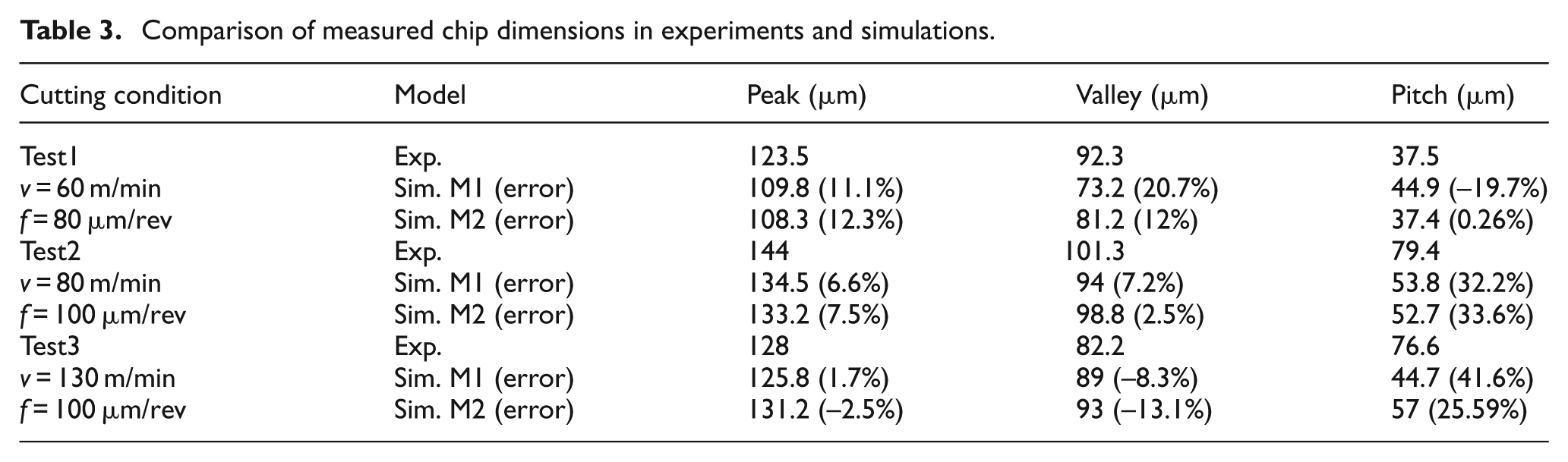
The average peak dimensions of M1 and M2 agree well with the experimental results in Tests 1 to 3, with relative errors lower than 15%, and they are similar with each other. The errors between the predicted (M1 and M2) and experimental valley dimensions (in Tests 1 to 3) are also lower than 15%, except for M1 (20.7% in Test 1). The predicted valley of the M2 model is closer to the experimental results than that of the M1 model in Tests 1 and 2. In addition, the average valley dimension of M1 is smaller than that of M2. This phenomenon may be caused by the material plastic flow along the shear bands. The density of material ductile failure energy

Comparing with the peak and valley dimensions, larger relative errors exist for the pitch dimension, as illustrated in the results of Tests 2 and 3. The pitch dimensions of model M2 are closer to the experimental results than those of M1, except Test 2. Although there is no distinct difference between M1 and M2 in the prediction of peak and valley dimensions, the pitch sizes of M2 are closer to the experimental results than those of M1. Thus, the optimized J–C model M2 is more appropriate to be applied in the titanium alloy machining simulation.
The predicted (M1 and M2) and experimental principle cutting forces of Tests 1 to 3 are shown in Figure 12. The predicted forces of M1 are larger than the experimental results, contrary to the relatively small predicted forces of M2. Based on the stress–strain curves of M1 and M2 models (Figure 8), higher stress will lead to a higher cutting force in the same FE model under the same strain condition. Although the predicted forces using M1 are closer to the experimental results, the errors of Tests 1 to 3 are 6.8%, 5.7% and 7.9%, respectively, the errors between M2 and experiment are lower than 15% (12.9%, 13.3% and 10.2% for Tests 1 to 3, respectively). As the measurement error and the differences of material physical behavior exist in the FE model and actual machining, the predicted forces can be considered as reasonable for model M1 and M2.
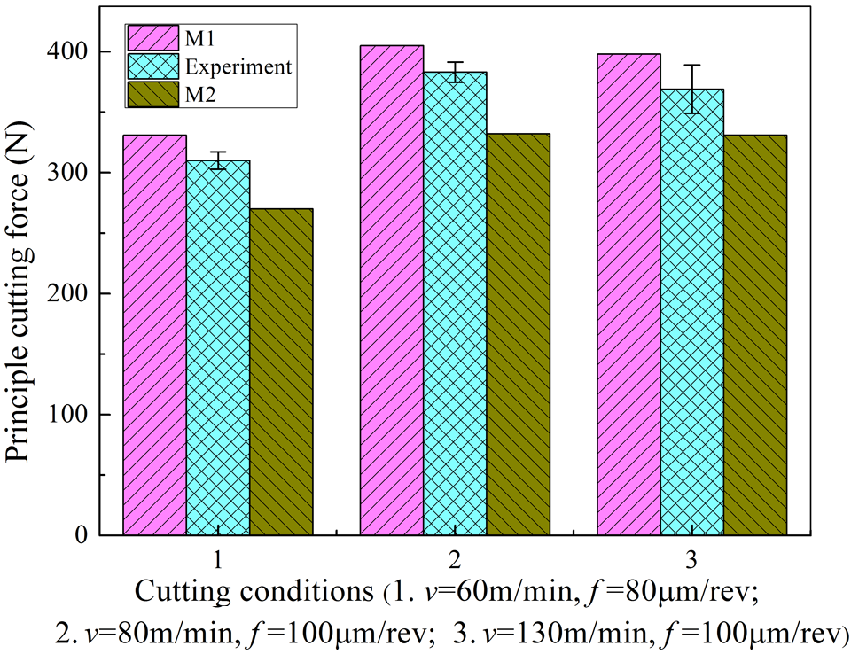
The predicted (with model M1 and M2) and experimental principle cutting forces.
Conclusions
A genetic algorithm was proposed to minimize the errors between the flow stress obtained through the J–C constitutive model parameters and the SHPB experimental results in Lee and Lin 14 at different temperatures (25 °C to 1100 °C) and high strain rates (2000 and 2500 s−1). In addition, Ti–6Al–4V alloy orthogonal cutting experiments and the corresponding FE simulations were performed to validate the optimized J–C model parameters. In summary, the following conclusions can be drawn.
The GA technique can be applied to minimize the difference between experimental and calculated material flow stress.
The flow stress obtained through the optimized J–C model M2 is closer to the experimental data than that of model M1. The percentage differences between the flow stress of the J–C model M2 and the experimental data at 2000 and 2500 s−1 are lower than 4% and 3%, respectively. Therefore, the flow stress obtained through the J–C model at different temperatures and strain rates can characterize the material flow stress obtained in the SHPB tests.
The experimental chip morphology and the FE simulation results obtained by the two sets of the J–C model (M1 and M2) showed no distinct difference between models M1 and M2 for peak and valley dimensions. In addition, the valley dimension of the segmented chip is greatly dependent on the J–C model parameters. At a constant density of material ductile failure energy in the material failure process, higher stress will lead to a shorter failure process, and thus cause a smaller valley dimension. The predicted pitch dimensions of the J–C model M2 are closer to the experimental results than those of M1. Thus, the GA-optimized material parameters M2 are more appropriate for the simulation of the titanium alloy machining process than model M1.
The percentage errors between the predicted (M1 and M2) and experimental principle cutting forces are lower than 15%. Hence, the predicted forces can be regarded as reasonable for both M1 and M2 models.
The optimized J–C model M2, which considers different temperatures (25 °C to 1100 °C) and strain rates (2000 and 2500 s−1), can be used to characterize the Ti–6Al–4V alloy deformation mechanism in machining simulation.
Footnotes
Appendix
Acknowledgements
The authors gratefully thank Mr Yang Lijian for his support in developing the optimization model.
Funding
This research was supported by the National High Technology Research and Development (863) Program of China [Grant No. 2008AA042509].
Conflict of interest
The authors declare that there is no conflict of interest.