Geometric error reduction in the assembly of axi-symmetric rigid components: a two-dimensional case study

Abstract

In this article, the assembly of axi-symmetric rigid structures from imprecisely manufactured components is considered to produce a ‘straight-build’ assembly. The eccentricity of the assembly is improved by selecting the best relative orientation of each component and using four different strategies to control the assembly errors. The presentation is simplified by considering the assembly of two-dimensional structures, and the Monte Carlo simulation technique is used to quantify the propagation of random component variations on the resulting assembly. The axial and radial run-outs for each component are used to represent component variability and these quantities are represented as Gaussian random variables. The influence of component variations on the assembly is predicted using connective assembly models. Numerical results are presented for assemblies consisting of: (a) identical rectangular components; and (b) non-identical rectangular components. The results are compared with each other and those obtained using ‘direct-build’ assembly, which does not control the assembly errors. It is found that assembly variations can be reduced significantly using the proposed techniques.

Introduction

The assembly of mechanical components has a significant impact on manufacturing cost and plays an important role in the quality of the final product. The quality of the assembly is greatly influenced by the presence of manufacturing variations in its constituent parts, and analysing and controlling the propagation of these variations through the assembly forms the main theme of this work.

Various methods have been used to predict the effect of component variations on mechanical assembly, and a detailed review of tolerance analysis can be found in Chase and Greenwood, ¹ Chase and Parkinson, ² and Marziale and Polini. ³ In most of these works, vector loop models are used to predict the propagation of variations through the assembly to assess its quality. Veitschegger and Wu ⁴ presented an analysis to predict the effect of individual link and joint errors on the three-dimensional (3D) kinematics of robotic systems. Jastrzebski ⁵ generalised this work and applied it to the travelling of mechanical assemblies, and Whitney et al.^6,7 extended it to represent feature and mating errors using connective models based on homogeneous matrix transforms. All of this work was used to analyse assembly variations at the conceptual design stage, but no effort was made to control the propagation of the variations through the assembly.

Mantripragada and Whitney ⁸ used state transition models to predict variation propagation in mechanical assemblies and proposed a statistical control theory to minimise assembly error. This control theory concentrates on designing the mating features so as to make adjustments possible during assembly. The proposed control theory can only be applied at the conceptual design stage. State space models have been used in Ding et al. ⁹ and Camelio et al. ¹⁰ to calculate variation propagation in a multi-station assembly system while considering part, process, and tooling variations. These articles focus on controlling variation propagation stage-by-stage using fixture adjustment. Reducing variation propagations in assembly has also been studied by various researchers.^11,12 These works use measured data for each component, along with in-line measurement, to monitor assembly variation to determine the required tooling correction to compensate assembly variation. Assembly of non-rigid sheet metal components were evaluated in these articles. Dantan et al. ¹³ proposes an integrated tolerancing process (ITP) that provides general methods and tools for reducing geometric variations in assembled products at the conceptual design stage.

Selective assembly is another approach to minimising assembly variations, and is based on using measurement data for components.^14–16 In this approach, mating components are measured and their measurement data grouped into ‘bins’. The components are assembled together by selecting components from the grouped data in order to meet the required specifications as closely as possible. The main limitation of this approach is that, in practice, it can only be applied to two-component assemblies in mass or batch production. Turner ¹⁷ and Li and Roy ¹⁸ have formulated a mathematical programming approach to find the optimal configuration of parts using a relative positioning technique based on geometric positioning of mating features of the part and the neighbouring parts. However, this approach cannot be applied to the assembly of rotating machines, where the mating components can only be rotated relative to each another.

This article focuses on the assembly of rotating machines consisting of nominally axi-symmetric components that need to satisfy strict balancing requirements. The presence of manufacturing variations in each component causes the mating features to have imperfect shape, orientation, and position, ¹⁹ and these geometric variations can significantly influence the quality of the final product. Rotating machines are commonly used in industry, including machining tools, industrial turbo-machinery, and aircraft engines. Vibration resulting from out-of-balance is the main factor that affects the reliability of high-speed rotating machines, and if the geometric axis of the assembled rotor is not built so that it is straight, the rotor may suffer from excessive vibration. ²⁰ In such cases, the goal is to build the assembly in such a manner that the geometric axis of the rotor is maintained as straight as possible. This can be achieved by controlling geometric variation propagation during assembly to ensure the build is as straight as possible, and this method of assembly is known as ‘straight-build’ assembly.

Key characteristics (KCs) ²¹ are used to identify the variations that most significantly affect product quality and the product features and tolerances that require special attention. The KC used to achieve a straight-build is the eccentricity of the assembly, and the main objective of this work is to minimise the overall eccentricity of the assembly to prevent deviation in the geometric axis of assembly. The process of straight-build assembly is usually divided into two steps.

1. Predict variation propagation at each assembly stage.

2. Control variation propagation in the assembly.

Step 1 requires a model to quantify propagation of component variations through the assembly based on detailed geometric data for all components, while Step 2 requires the predicted assembly variations to be reduced using an optimisation strategy.

The model used here to predict variation propagation is based on connective assembly models.^6,22 These models use homogeneous matrix transforms ²³ that define the geometric relationship between different features on the same component and neighbouring components. In a practical implementation, measurements can be made to determine the geometry of the components and assembly features at each stage. In this article, the geometric data is randomly generated based on the predefined geometric tolerances of individual components and the geometry of the assembly is calculated accordingly. Four control (optimisation) methods are proposed to reduce assembly variation. Details of these methods are presented later, but all make use of the axi-symmetric property of the assembly and allow each component to be orientated relative to its neighbour to better achieve a straight-build assembly. In practice, only particular ‘indexed’ orientations are allowed and the optimal orientation is obtained by minimising a suitable objective function.

Throughout the article, the analysis and numerical examples are developed in two dimensions (2D) to allow the reader to visualise and understand the calculations performed more easily. Two assembly examples are studied to compare the different optimisation techniques.

1. Assembly of identical rectangular components.

2. Assembly of non-identical rectangular components.

The component variations considered are based on industrial measurement practice and the Monte Carlo simulation technique is used to simulate variation propagation and evaluate the performance of the proposed optimisation methods to control straight-build assembly. For the purposes of comparison, results are also obtained using ‘direct-build’ assembly, which does not use any optimisation.

Representing component variations

For the purpose of simplification, the (rigid) axi-symmetric components considered here are 2D nominally rectangular components. Figure 1(a) shows the nominal geometry of one of the rectangular components having width B and height H. In essence, the assembly process consists of ‘stacking’ one rectangular component on top of another to build a tower. In practice, manufacturing variations are present and these are often defined in terms of a tolerance zone. Run-out tolerances are usually applied to parts that rotate about an axis of rotation, which constitutes a datum. Run-out tolerance controls the deviation of part features relative to the axis of rotation and is an important tolerance specification for axially symmetric parts. It represents the cumulative effects of form, position, and orientation tolerances ²⁴ and, therefore, takes into account variations such as form, location, and orientation. When applied to features constructed around a datum axis, run-out also controls the cumulative variations of circularity and concentricity. ²⁵ When applied to features constructed perpendicular to a datum axis, run-out controls variations in the circular element of a plane surface to detect wobble or surface irregularities. According to BS EN ISO 1101:2005, ²⁶ run-out not only applies to complete features, but can also be applied to a restricted area of the feature. Run-out tolerance that applies to a complete feature is called total run-out and that applies to a restricted feature (circular element of a feature) is called circular run-out. One of the aims of this article is to evaluate the effect of radial and axial run-out (circular) tolerances on the assembly variation propagation. The tolerance zones for radial run-out (circular) and axial run-out (circular) as defined in BS EN ISO 1101:2005 ²⁶ applied to a 2D case are shown in Figure 1(a). These zones indicate the tolerances for variation of the top surface in the axial direction (i.e. along the datum axis) and the sides of the rectangle in the radial direction (i.e. perpendicular to datum axis). The radial run-out shall not be greater than b at any instance in a direction perpendicular to the datum axis and axial run-out shall not be greater than h at any position on the top surface.

Figure 1.

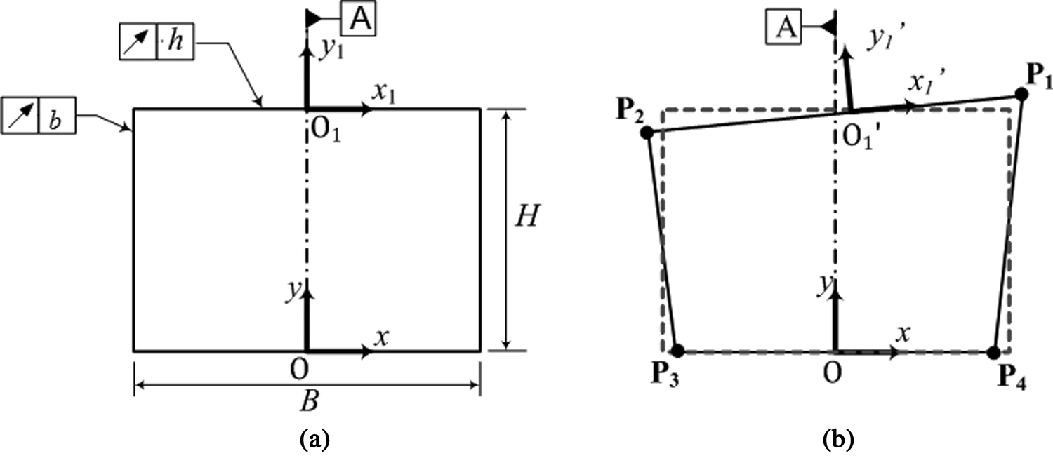
(a) Nominal rectangular component with tolerance zone indicated. (b) Manufactured ‘rectangular’ component.

Figure 1(b) shows the geometry of a sample manufactured component where it can clearly be seen that the geometry deviates from the nominal. The geometry of the manufactured component shows that corner points ${\text{P}}_1$ , ${\text{P}}_2$ , ${\text{P}}_3$ , and ${\text{P}}_4$ , are dislocated from their nominal position. Dislocation of corner points ${\text{P}}_1$ and ${\text{P}}_2$ produces errors in the location and orientation of the top ‘mating’ surface ${\text{P}}_1{\text{P}}_2$ (which may be in contact with another component) with respect to base ( ${\text{P}}_3{\text{P}}_4$ ) of the rectangle.

For the purpose of travelling the propagation of component variations through an assembly, coordinate axes $\text{O}\mathrm{xy}$ and ${\text{O}}_1\prime x_1\prime y_1\prime$ (see Figure 1(b)) are attached to the manufactured component to define the location and orientation of the mating features at which the components are joined. The origins $\text{O}$ and ${\text{O}}_1\prime$ are chosen to lie midway across the upper and lower surfaces of the component, while the $\text{O}x$ and ${\text{O}}_1\prime x_1\prime$ axes are chosen to be parallel with the lower and upper surfaces of the component respectively (see Figure 1(b)).

In industrial applications, the geometry of a manufactured component can be measured before the assembly process starts. For example, in the assembly of high-value axi-symmetric components, each component can be measured using fixed measurement probes to determine the radial run-out (circular) and axial run-out (circular) of the mating features from the nominal. Figure 2 indicates the measurements performed for a 2D component, and these are described below.

Figure 2.

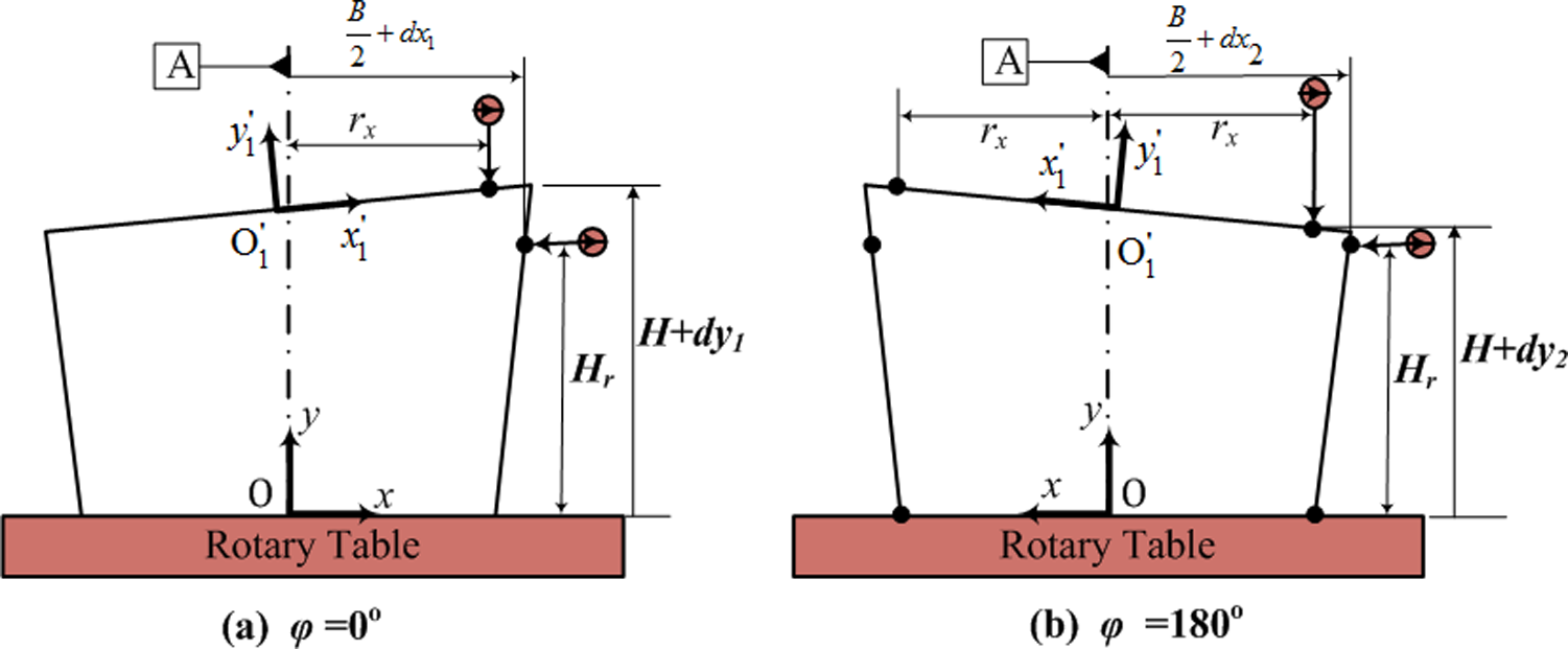
Measurement of component variation.

Each component is placed on a rotary table so that the lower mating surface of the component is concentric with the central axis of the rotary table – the so-called ‘table-axis’. ²⁷ This ensures that the component reference frame is attached to the centre of the base of the component and coincides with the global reference frame on the table. For the top surface of the component, the axial length is measured at fixed radius $r_x$ to determine the axial run-out. For the sides of the component, the radius is measured at fixed height $H_r$ to determine the radial run-out. In practice, the fixed radius and fixed height are chosen so that the measurements are made as close as practically possible to the corners of the component. Although this introduces small errors into the measurements, these errors are negligible compared with the variations considered here. All axial and radial run-out (circular) measurements are made using a fixed measurement probe that takes measurements on the surface of a nominally circular component as the part makes one complete revolution about the datum axis, owing to rotation of the rotary table. ²⁵ For a 3D axi-symmetric component, measurements are made for the radial and axial run-outs. A best circle is fitted to the measured radial run-out measurements and this circle is used to identify the shift in the actual centre of the circular feature compared with the nominal centre. The best plane is fitted to the measured axial run-out measurements and this circle is used to identify the net effect of the surface irregularities. For the 2D components considered here, only two measurements are possible for both radial and axial run-outs. The first measurement is made when $\phi =0^{\circ }$ (Figure 2(a)), while the second measurement is made after the table has been rotated through $\phi ={180}^{\circ }$ (Figure 2(b)).

Mathematically, the radial run-out can be expressed using polar coordinates as

$$R\left(\phi \right)=\frac{B}{2}+r_{\mathrm{run}-\mathrm{out}}(\phi )$$

(1)

where $R\left(\phi \right)$ is the radius of a point on the measured surface at table orientation $\phi$ , $\frac{B}{2}$ is the nominal radius, and $r_{\mathrm{run}-\mathrm{out}}\left(\phi \right)$ is the measured run-out in the radial direction.

Similarly, the axial run-out can be expressed in polar coordinates as

$$H\prime \left(\phi \right)=H+a_{\mathrm{run}-\mathrm{out}}(\phi )$$

(2)

where $H\left(\phi \right)$ is the height of the measured point at table orientation $\phi$ , $H$ is the nominal height of the feature, and $a_{\mathrm{run}-\mathrm{out}}(\phi )$ is the measured value of run-out in the axial direction.

Manufacturing variations are commonly assumed to have a normal (Gaussian) distribution with mean equal to the nominal size and the range of variation equal to six standard deviations ( $\pm 3\text{σ}$ ).^2,28,29 For axi-symmetric assemblies, like those considered in the examples section, the radial and axial run-outs for the nominal assembly are zero, so the radial and axial run-out variations are assumed to be zero-mean Gaussian random variables. Given that machining operations to manufacture axi-symmetric components typically involve different operations to produce the circular shape and flat surfaces at either end, it is justifiable to assume that axial and radial run-outs are independent of each other. Therefore, in this study, radial and axial run-out variations are generated randomly at the two table orientations by assuming they are independent Gaussian random variables having standard deviations σr and σa, respectively. The values of σr and σa are chosen based on the specified tolerance and assume that the tolerance limits coincide with the ‘±3σ’ limits of a Gaussian distribution. This is based on the fact that 99.73% of random data chosen from a Gaussian distribution falls within the ±3σ range about the mean.^30,31

If the radial run-out at corner ${\text{P}}_1$ is $\frac{B}{2}+d{x}_1$ and the axial height at corner ${\text{P}}_1$ is $H+d{y}_1$ , then the global co-ordinates of corner ${\text{P}}_1$ are $(\frac{B}{2}+d{x}_1,H+d{y}_1)$ . Similarly, if the radial run-out at corner ${\text{P}}_2$ is $\frac{B}{2}+d{x}_2$ and the axial height at point ${\text{P}}_2$ is $H+d{y}_2$ , then the global co-ordinates of corner ${\text{P}}_2$ are ( $-\frac{B}{2}-d{x}_2$ , $H+d{y}_2$ ).

To model the propagation of component variations through an assembly, it is necessary to specify the location of coordinate frame ${\text{O}}_1\prime x_1\prime y_1\prime$ relative to coordinate frame ${\text{O}}_1{x}_1{y}_1$ (see Figure 1). For the nominal component, the global co-ordinates of origin ${\text{O}}_1$ are $(0,H)$ . For the manufactured component, the co-ordinates of origin ${\text{O}}_1\prime$ are $(\mathrm{dx},H+\mathrm{dy})$ , where $\mathrm{dx}$ is the deviation of origin ${\text{O}}_1\prime$ in the x-direction and $\mathrm{dy}$ is the deviation of origin ${\text{O}}_1$ in the y-direction. Figure 3 shows an enlarged view of the top surface of the component shown in Figure 2 and is used to determine the relationship between $\mathrm{dx}$ , $\mathrm{dy}$ , $d{x}_1$ , $d{x}_2$ , $d{y}_1$ , and $d{y}_2$ . Noting that origin ${\text{O}}_1$ lies midway between corners ${\text{P}}_1$ and ${\text{P}}_2$ and using Figure 3, it can be shown easily that

$$\mathrm{dx}=\frac{d{x}_1-d{x}_2}{2}$$

(3)

$$\mathrm{dy}=\frac{d{y}_1+d{y}_2}{2}$$

(4)

Figure 3.

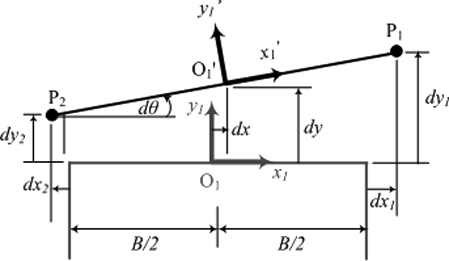
Enlarged view of top surface measurement.

In equations (3) and (4), it should be noted that $\mathrm{dx}$ is a function of radial run-out variations $d{x}_1$ and $d{x}_2$ only, while $\mathrm{dy}$ is a function of axial run-out variations $d{y}_1$ and $d{y}_2$ only. This ensures that $\mathrm{dx}$ and $\mathrm{dy}$ are independent of each other.

The measured coordinates of ${\text{P}}_1$ and ${\text{P}}_2$ can also be used to determine the orientation of coordinate frame ${\text{O}}_1\prime x_1\prime y_1\prime$ relative to coordinate frame ${\text{O}}_1{x}_1{y}_1$ . Using Figure 3 it can easily be shown that the relative orientation $d\theta$ is defined as

$$\tan d\theta =\frac{d{y}_1-d{y}_2}{B+d{x}_1+d{x}_2}$$

(5)

In equation (5) it is shown that $d\text{θ}$ is a function of radial run-out ( $d{x}_1$ and $d{x}_2$ ) and axial run-out ( $d{y}_1$ and $d{y}_2$ ) only, this indicates that angular orientation error $d\text{θ}$ is dependent on both radial and axial run-outs.

The work presented in this section describes how manufacturing variations in axi-symmetric components can be represented in terms of axial and radial run-outs. The locations of corners ${\text{P}}_1$ and ${\text{P}}_2$ (see Figure 2) are simulated by assuming that the coordinates of each point are independent Gaussian random variables, i.e. $d{x}_1$ , $d{x}_2$ , $d{y}_1$ , and $d{y}_2$ are independent zero-mean Gaussian random variables with known standard deviation. These coordinates are used to determine the location and orientation of the component mating feature, which are defined in terms of the nominal geometry of the component and $\mathrm{dx}$ , $\mathrm{dy}$ , $d\theta$ (see equations (3), (4), and (5)). This data is used in the connective assembly model described in the following section to quantify the influence of component variations on the eccentricity of the assembly.

Variation propagation model

To study and analyse assembly related problems, it is essential to develop an appropriate assembly model that allows each component and the resulting assembly to be represented mathematically. Connective assembly models are used here to quantify variation propagation in the assembly. In these models, matrix transformations are used to relate the location and orientation of different features on a component. Here, this approach is particularly useful for considering the relationship between mating features on the same and different components. This is achieved by attaching coordinate frames to each of the mating features and considering the geometric relationship between them. Each coordinate frame is described in terms of its position and orientation, and for an assembly containing manufactured components, the position and orientation of the coordinate frame is affected by manufacturing variations (see equations (3), (4), and (5)).

For 2D components the geometric relationship between any two coordinate frames can be depicted as shown in Figure 4. In Figure 4, the geometric relationship between coordinate frame U and coordinate frame V is represented using transformation matrix $\mathbf{T}$ . The transformation matrix represents the operations of translation and rotation acting on a coordinate frame originally aligned with a reference coordinate frame, ²³ and is given by

$$\mathbf{T}=\left[\begin{array}{cc}\hfill \mathbf{S}\hfill & \hfill \mathbf{p}\hfill \\ \multicolumn{1}{c}{0^T}& \hfill 1\hfill \end{array}\right]$$

(6)

where $\mathbf{S}$ and $\mathbf{p}$ are given by

$$\mathbf{S}=\left[\begin{array}{cc}\hfill \cos \theta \hfill & \hfill -\sin \theta \hfill \\ \multicolumn{1}{c}{\sin \theta }& \hfill \cos \theta \hfill \end{array}\right]$$

(7)

$$\mathbf{p}=\left[\begin{array}{c}\hfill X\hfill \\ \multicolumn{1}{c}{Y}\end{array}\right]$$

(8)

Figure 4.

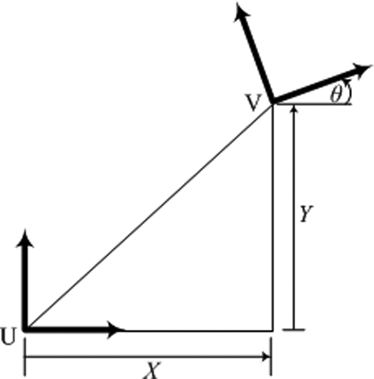
Geometric relationship between two coordinate frames.

The symbols X, Y, and θ are defined in Figure 4, and represent origin translation (X and Y) and rotation θ. Matrix $\mathbf{S}$ indicates the orientation of coordinate frame V relative to coordinate frame U, while vector $\mathbf{p}$ is a $2\times 1$ displacement vector indicating the location of the origin of coordinate frame V relative to the origin of coordinate frame U.

The assembly model assumes that components are assembled by joining mating features to each other ³² and transformation matrices are used to relate the location of mating features. Figure 5 shows a two-component assembly. In this assembly, the mating features are defined by coordinate reference frames: ${\text{O}}_0{x}_0{y}_0$ , ${\text{O}}_1{x}_1{y}_1$ , ${\text{O}}_2{x}_2{y}_2$ , and ${\text{O}}_3{x}_3{y}_3$ , where ${\text{O}}_0{x}_0{y}_0$ is chosen to represent the global reference frame. The assembly consists of joining coordinate frame ${\text{O}}_1{x}_1{y}_1$ on part A to coordinate frame ${\text{O}}_2{x}_2{y}_2$ on part B, and composing matrix transformations to express the component-to-component relationships. Figure 5 depicts the nominal case, where no manufacturing variations are present. For this situation, the transformation matrix ${\mathbf{T}}_{0-1}^N$ between features 0 and 1 on nominal Part A can be expressed as

$${\mathbf{T}}_{0-1}^N=\left[\begin{array}{cc}\hfill {\mathbf{S}}_A^N\hfill & \hfill {\mathbf{p}}_A^N\hfill \\ \multicolumn{1}{c}{{\mathbf{0}}^T}& \hfill 1\hfill \end{array}\right]$$

(9)

Figure 5.

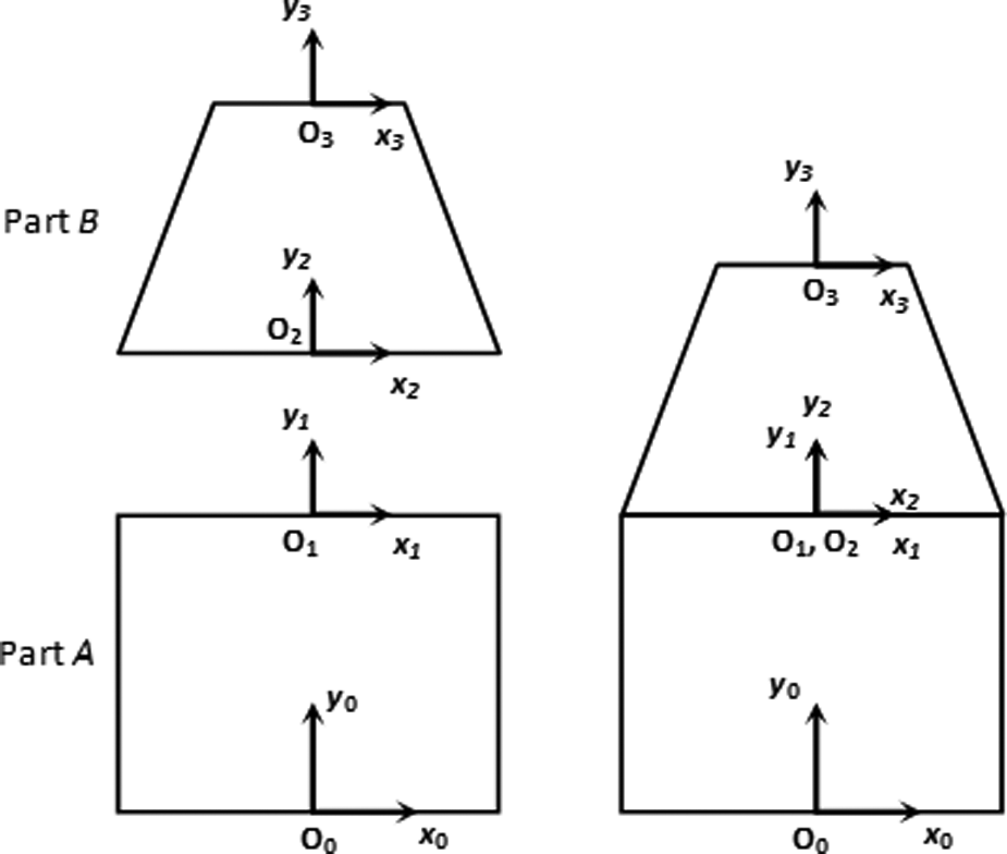
An example of two component assembly.

This transformation has the same form as equation (6), where ${\mathbf{S}}_A^N$ is a $2\times 2$ matrix indicating the nominal orientation of frame 1 relative to frame 0, and ${\mathbf{p}}_A^N$ is a $2\times 1$ displacement vector indicating the nominal location of origin ${\text{O}}_1$ relative to origin ${\text{O}}_0$ on Part A. The superscript N indicates that the transformation matrix relates to the nominal geometry of the component.

Similarly, transformation matrix ${\mathbf{T}}_{2-3}^N$ between features 2 and 3 on nominal Part B can be expressed as

$${\mathbf{T}}_{2-3}^N=\left[\begin{array}{cc}\hfill {\mathbf{S}}_B^N\hfill & \hfill {\mathbf{p}}_B^N\hfill \\ \multicolumn{1}{c}{{\mathbf{0}}^T}& \hfill 1\hfill \end{array}\right]$$

(10)

where ${\mathbf{S}}_B^N$ is a $2\times 2$ matrix indicating the nominal orientation of frame 3 relative to frame 2, and ${\mathbf{p}}_B^N$ is a $2\times 1$ displacement vector indicating the nominal location of origin ${\text{O}}_3$ relative to origin ${\text{O}}_2$ on Part B.

When Parts A and B are assembled together (see Figure 5), transformation matrix ${\mathbf{T}}_{0-3}^N$ between feature 0 on Part A and feature 3 on Part B can be expressed using the properties of the transformation matrices ²² to give

$${\mathbf{T}}_{0-3}^N={\mathbf{T}}_{0-1}^N{\mathbf{T}}_{1-2}^N{\mathbf{T}}_{2-3}^N$$

(11)

where transformation matrix ${\mathbf{T}}_{1-2}^N$ is the transformation matrix between nominal connecting feature 1 on Part A and feature 2 on Part B. Provided that coordinate frames ${\text{O}}_1{x}_1{y}_1$ and ${\text{O}}_2{x}_2{y}_2$ are coincident, ${\mathbf{T}}_{1-2}^N$ is a $3\times 3$ identity matrix. ${\mathbf{T}}_{0-3}^N$ can be expressed in the same form as equations (6), (9), and (10), such that

$${\mathbf{T}}_{0-3}^N=\left[\begin{array}{cc}\hfill {\mathbf{S}}_{\mathrm{AB}}^N\hfill & \hfill {\mathbf{p}}_{\mathrm{AB}}^N\hfill \\ \multicolumn{1}{c}{{\mathbf{0}}^T}& \hfill 1\hfill \end{array}\right]$$

(12)

where ${\mathbf{S}}_{\mathrm{AB}}^N$ is a 2 × 2 matrix indicating the nominal orientation of frame 3 relative to frame 0, and ${\mathbf{p}}_{\mathrm{AB}}^N$ is a 2 × 1 displacement vector indicating the nominal location of origin ${\text{O}}_3$ relative to origin ${\text{O}}_0$ . Comparing the entries in equation (12) with equations (7) and (8), the equivalent displacement coordinates and relative orientation between reference frames ${\text{O}}_0{x}_0{y}_0$ , and ${\text{O}}_3{x}_3{y}_3$ can be calculated.

Equations (9)–(12) are the transformation matrices for an assembly consisting of two nominal components (Parts A and B in Figure 5). These transformation matrices must be modified to take account of manufacturing variations in each component, and this can be done by incorporating variations into the position and orientation of the coordinate frames attached to the mating features. For example, manufacturing variations in Part A may modify the location and orientation of frame 1 relative to frame 0, such that transformation matrix ${\mathbf{T}}_{0-1}$ can be approximated as

$${\mathbf{T}}_{0-1}={\mathbf{T}}_{0-1}^N{\mathbf{D}}_A$$

(13)

where ${\mathbf{T}}_{0-1}^N$ is given by equation (9) and

$${\mathbf{D}}_A=\left[\begin{array}{ccc}\hfill 1\hfill & \hfill -d\theta \hfill & \hfill \mathrm{dx}\hfill \\ \multicolumn{1}{c}{d\theta }& \hfill 1\hfill & \hfill \mathrm{dy}\hfill \\ \multicolumn{1}{c}{0}& \hfill 0\hfill & \hfill 1\hfill \end{array}\right]$$

(14)

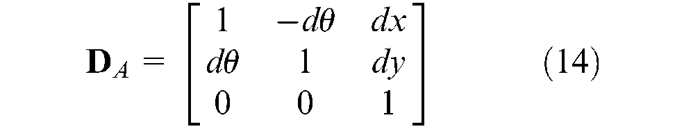
Equation (14) is based on equations (6)–(8) and assumes that $\mathrm{dx}$ , $\mathrm{dy}$ , and $d\theta$ are small. Transformation matrix ${\mathbf{D}}_A$ effectively takes account of the manufacturing variations present in Part A.

Similarly, the presence of manufacturing variations in Part B will modify the location and orientation of frame 3 relative to frame 2, and transformation matrix ${\mathbf{T}}_{2-3}$ relating frame 3 to frame 2 can be expressed as

$${\mathbf{T}}_{2-3}={\mathbf{T}}_{2-3}^N{\mathbf{D}}_B$$

(15)

where ${\mathbf{T}}_{2-3}^N$ is given by equation (10) and transformation matrix ${\mathbf{D}}_B$ has a similar form to equation (14).

If Parts A and B are assembled together, the transformation matrix ${\mathbf{T}}_{0-3}$ between feature 0 on Part A and feature 3 on Part B, taking into account manufacturing variations can be expressed as

$${\mathbf{T}}_{0-3}={\mathbf{T}}_{0-1}{\mathbf{T}}_{1-2}{\mathbf{T}}_{2-3}$$

(16)

where transformation matrix ${\mathbf{T}}_{1-2}$ is the transformation matrix between connecting features. As discussed previously, this transformation matrix is the identity matrix if the mating features are coincident. If assembly errors are present, then a transformation matrix, having an identical form to equation (14), can be used to represent ${\mathbf{T}}_{1-2}.$

Using equation (16), ${\mathbf{T}}_{0-3}$ can be expressed in the same form as equation (6), such that

$${\mathbf{T}}_{0-3}=\left[\begin{array}{cc}\hfill {\mathbf{S}}_{\mathrm{AB}}\hfill & \hfill {\mathbf{p}}_{\mathrm{AB}}\hfill \\ \multicolumn{1}{c}{0^T}& \hfill 1\hfill \end{array}\right]$$

(17)

where ${\mathbf{S}}_{\mathrm{AB}}$ is a $2\times 2$ matrix indicating the actual orientation of frame 3 relative to frame 0, and ${\mathbf{p}}_{\mathrm{AB}}$ is a $2\times 1$ displacement vector indicating the actual location of origin ${\text{O}}_3$ relative to origin ${\text{O}}_0$ . Comparing equation (17) with equation (6), it is quite straightforward to calculate the equivalent displacement coordinates and relative orientation between reference axes ${\text{O}}_0{x}_0{y}_0$ and ${\text{O}}_3{x}_3{y}_3$ , taking manufacturing variations into account. The translation error between the actual assembly ${\mathbf{p}}_{\mathrm{AB}}$ and the nominal assembly ${\mathbf{p}}_{\mathrm{AB}}^N$ can be used to quantify the influence of component manufacturing and joining variation on the assembly, where the translational error vector $({\mathrm{dp}}_{\mathrm{AB}}^x,{\mathrm{dp}}_{\mathrm{AB}}^y)$ is given by

$$\left[\begin{array}{c}\hfill {\mathrm{dp}}_{\mathrm{AB}}^x\hfill \\ \multicolumn{1}{c}{{\mathrm{dp}}_{\mathrm{AB}}^y}\end{array}\right]={\mathbf{p}}_{\mathrm{AB}}-{\mathbf{p}}_{\mathrm{AB}}^N$$

(18)

In this section, a method of quantifying variation propagation in mechanical assemblies has been presented and illustrated for the case of a two component assembly. This approach can be extended easily to consider more components and forms the basis for the calculations performed in later sections.

Straight-build assembly optimisations

To improve the quality of the assembly and increase the likelihood of ‘right first time’ assembly, it is essential to reduce and control assembly errors. Optimisation is used in many fields of engineering to minimise or maximise a function critical to the problem being solved.^33,34 The optimisation methods used here aim to achieve straight-build assembly and involve selecting an optimal relative orientation between axi-symmetric components to reduce assembly errors. Four optimisation methods are suggested here to minimise error propagation in straight-build assembly.

Methods 1 to 3 each consider the table-axis error; that is, the perpendicular distance between the table-axis and the centre of a component. Method 4 considers the final-assembly axis error; that is the perpendicular distance between the assembly axis passing through the centre of the base of the first component and the centre of the final component in the assembly. Each method uses a relative orientation technique to minimise error propagation in the assembly. The relative orientation technique is a unique approach of error minimisation, where each part is oriented relative to its adjacent part by rotating it about its axis of symmetry. An optimal relative orientation between the mating components is selected based on the objective function for each optimisation method. Straight-build assembly is a useful approach for assembling rotating machines and is equally applicable to 2D and 3D assemblies. For 2D assembly, each new component has two possible orientations (0° or 180°) relative to the mating component in the assembly. However, for 3D assembly each new component can be oriented at any angular position (between 0°–360°) depending upon the method of joining two components in the assembly. Using 2D examples provides clear understanding of the proposed relative orientation techniques and demonstrates how the error minimisation process is applied to an assembly of axi-symmetric components (in rotating machines). The 2D example also allows the reader to visualise and understand the calculations performed more easily. No matter how the optimisation is performed for 2D assemblies (with two possible relative orientations) or 3D assembly (with a larger number of relative orientations), in both 2D and 3D the results will yield similar conclusions, because all optimisation methods consider the same number of relative orientations during assembly of each axi-symmetric component. Details of the proposed optimisation methods are given below.

Method 1: table-axis-build assembly (stage-by-stage optimisation)

In Method 1, the table-axis error is minimised at each stage of the assembly process by rotating the upper component about its axis of symmetry. Figure 6 shows a two-component assembly with the upper component in its two possible orientations. The table-axis error is the horizontal component of the translation error vector and is given by equation (18). In Figure 6, orientation 2 has a visibly smaller table-axis error than orientation 1 and is chosen as the optimal orientation.

Figure 6.

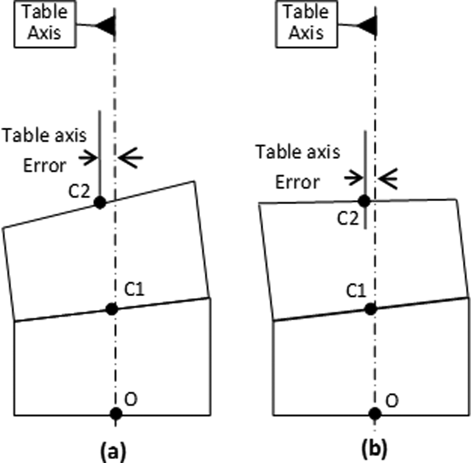
Method 1: two-component assembly with upper component in: (a) orientation 1, (b) orientation 2.

This optimisation process is performed at each stage of assembly as each new component is added to the assembly. Applying this process, the optimised table-axis error ${\epsilon }_i^{\mathrm{ota}}$ for the i’th component of the assembly is given by

$${\epsilon }_i^{\mathrm{ota}}=\underset{\phi =0^{\circ },{180}^{\circ }}{min}(|d{x}_i(\varphi )|)$$

(19)

where $|d{x}_i(\phi )|$ is the table-axis error for the i’th component at orientation $\phi$ .

Method 1 is basically a local combinatorial approach, providing a solution by making the best choice of all possible component orientation relative to the assembly during each stage.

Method 2: table-axis-build assembly (optimising error at two consecutive stages)

In method 2 the table-axis error is predicted for two subsequent stages by calculating the eccentricity for all four possible orientations of the two components. The optimal orientation is chosen as the configuration that minimises the combined error for the two stages considered. Using the notation introduced in method 1, the combined table-axis error is expressed as the root mean square (RMS) error for the two stages (i’th and (i+1)’st stages).

Applying this method, the optimised combined table-axis error ${\epsilon }_i^{\mathrm{ota}}$ for the i’th component of the assembly is given by

$${\epsilon }_i^{\mathrm{octa}}=\underset{\genfrac{}{}{0ex}{}{{\varphi }_{i1}=0^{\circ },{180}^{\circ }}{{\varphi }_{i2}=0^{\circ },{180}^{\circ }}}{min}\left(\sqrt{\frac{{|d{x}_i({\varphi }_{i1})|}^2+{|d{x}_{i+1}({\varphi }_{i2})|}^2}{2}}\right).$$

(20)

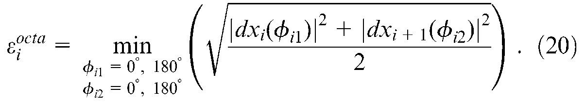
The orientations ${\phi }_{i1}={\alpha }_1$ and ${\phi }_{i2}={\alpha }_2$ that satisfy equation (20) define the optimal configuration. Using these values, the optimised table-axis error ${\epsilon }_i^{\mathrm{ota}}$ for the i’th component of the assembly is given by ${\epsilon }_i^{\mathrm{ota}}=|d{x}_i({\alpha }_1)|$ .

Method 3: table-axis-based combinatorial approach

In method 3, all possible orientations of all components in the assembly are considered, and the configuration of components that yields the minimum table-axis error for the whole assembly is chosen to be optimal.

Applying this method, the optimised table-axis error ${\epsilon }^{\mathrm{otaa}}$ for the whole assembly is calculated as

$${\epsilon }^{otaa}=\underset{\begin{array}{l}{\varphi }_1=0^{\circ },{180}^{\circ }\\ {\varphi }_2=0^{\circ },{180}^{\circ }\\ \dots \\ {\varphi }_N=0^{\circ },{180}^{\circ }\end{array}}{\min }\left(\sqrt{\frac{{\displaystyle \sum _{i=1}^N{\left|d{x}_i({\varphi }_i)\right|}^2}}{N}}\right).$$

(21)

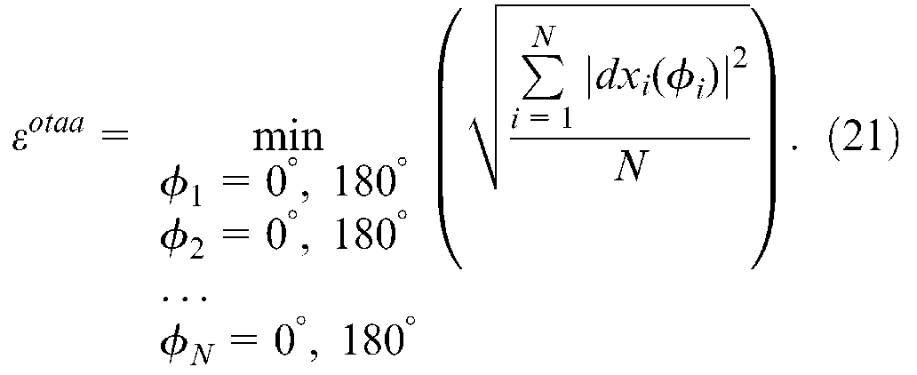
The orientations ${\phi }_i={\beta }_i$ that satisfy equation (21) define the optimal configuration. Using these values the optimised table-axis error ${\epsilon }_i^{\mathrm{ota}}$ for the i’th component of the assembly is given by

$${\epsilon }_i^{\mathrm{ota}}=|d{x}_i({\beta }_i)|$$

(22)

Method 4: final-assembly axis-based combinatorial approach

In method 4, a similar approach is applied to method 3, but instead of minimising the table-axis error for the whole assembly, method 4 minimises the final-assembly axis error. As defined earlier in the section ‘Straight-build assembly optimisations’, final-assembly axis refers to the axis passing through the centre of the base of the first component to the centre of top of the final component in the assembly.

Direct-build assembly

To investigate any potential improvements in straight-build assembly, the above four optimisation methods are compared with each other, and direct-build assembly. Direct-build assembly includes component variations but does not use any optimisation methods to control variation propagation.

Assembly examples to analyse proposed straight-build methods

Two examples are considered to investigate the performance of the proposed optimisation methods to improve straight-build assembly. Each of the assembly examples consists of axi-symmetric rigid components and the following assembly stages. The first stage of assembly is to place the first component on the table with its base concentric to the geometric centre of the table. As stated earlier, the point of coincidence of the centre of the base of the first component and the geometric centre of the table-axis is considered as the origin of the global coordinate frame. At each subsequent stage, a component is joined to the assembly by locating the mating features for the component so that it is concentric with the reference frame attached to the assembly feature.

Each component is assumed to contain geometric variation at the mating features, and the presence of geometric variations cause misalignment of the mating features of the component relative to the nominal situation. These variations accumulate as the parts are assembled together. In order to improve assembly quality, the four different optimisation methods are analysed.

The performance of the proposed optimisation methods is investigated using the standard Monte Carlo simulation approach. Convergence studies have been performed to determine the number of simulations required by Monte Carlo simulation to obtain accurate results. These studies involved determining the number of simulations required to obtain predictions for the mean and standard deviation that were accurate to within 1%. For the examples considered, approximately 50,000 simulations were required. In this approach, the axial and radial run-outs for each component ( $d{x}_1$ , $d{x}_2,$ $d{y}_1$ , $d{y_2}$) are selected to be independent zero-mean Gaussian random variables with known standard deviation based on specified tolerance data. Using equations (3), (4), and (5), these values are transformed into translation $(\mathrm{dx},\mathrm{dy})$ and rotation $(d\theta )$ errors for the reference frame defining the mating feature for the component. The reference frame data is then used in the connective assembly models described in section ‘Variation propagation model’ to build the assembly and calculate the assembly variations for each component from the table-axis (methods 1–3) or the final axis (method 4). In the connectivity models used, it has been assumed that there is no variation at the mating between any two components. Each assembly is repeated 50,000 times using the proposed optimisation methods and direct-build assembly, and statistical data for the resulting assembly errors are generated. To measure the variation in the complete (or part) assembly, the RMS variation for all components in the assembly is calculated. For an assembly consisting of N components, the RMS assembly variation from the table-axis ${\epsilon }_{\mathrm{ta}}^{\mathrm{RMS}}$ is calculated as follows

$${\epsilon }_{\mathrm{ta}}^{\mathrm{RMS}}=\sqrt{\frac{\sum _{i=1}^N{({\epsilon }_i^{\mathrm{ota}})}^2}{N}}$$

(23)

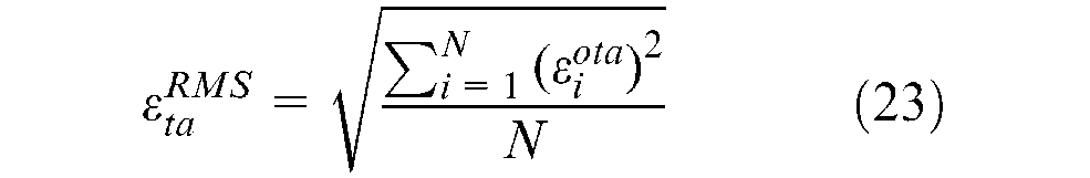
The RMS assembly variation from the final-assembly axis is calculated in a similar way, by replacing the table-axis error for each component by the final-assembly axis error in equation (23). In what follows, the statistical distribution, mean, and standard deviation of the assembly variation (mean of the RMS for 50,000 repeated assemblies) are presented for the complete assembly and at different stages of assembly.

Example 1: identical components assembly

This example investigates assemblies consisting of identical components. To analyse the performance of the proposed methods, assemblies with 4, 6, and 8 identical components are considered. Each component has a nominal width B = 100 mm and nominal height H = 70 mm. The geometric feature tolerances for axial and radial run-out of each component are assumed to be 0.1 mm and 0.05 mm, respectively.

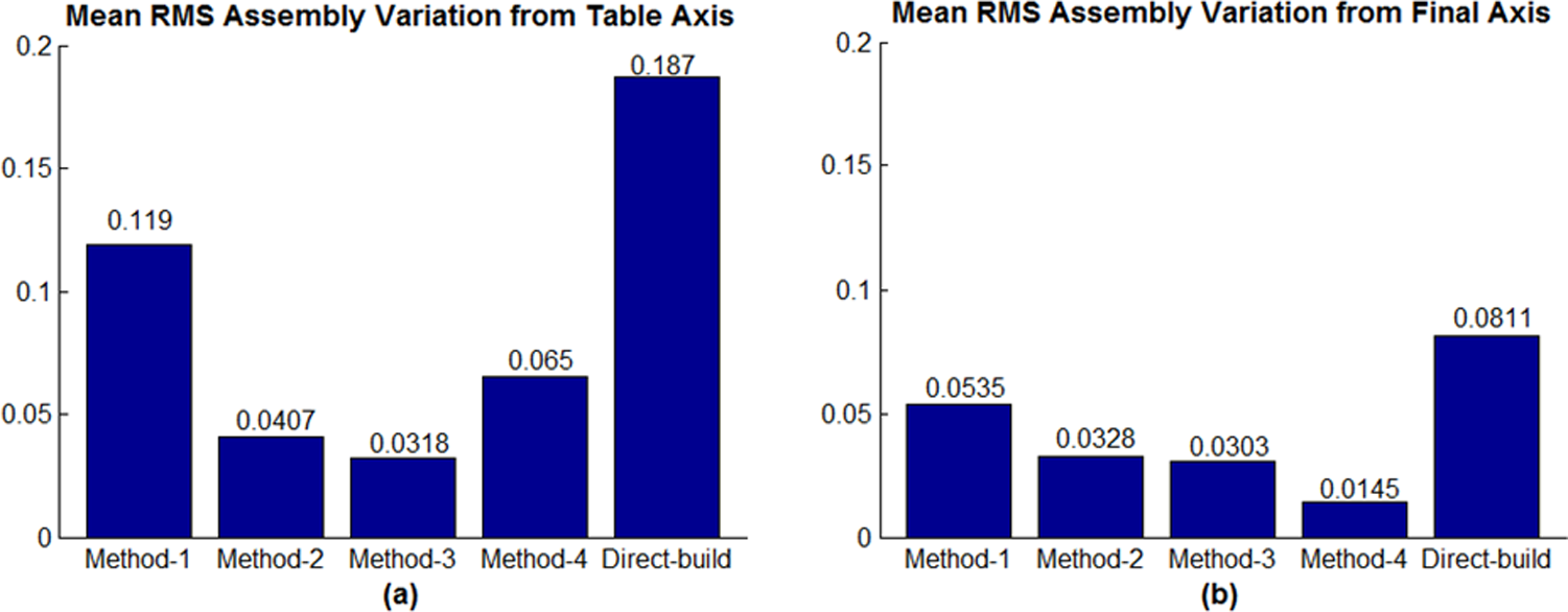
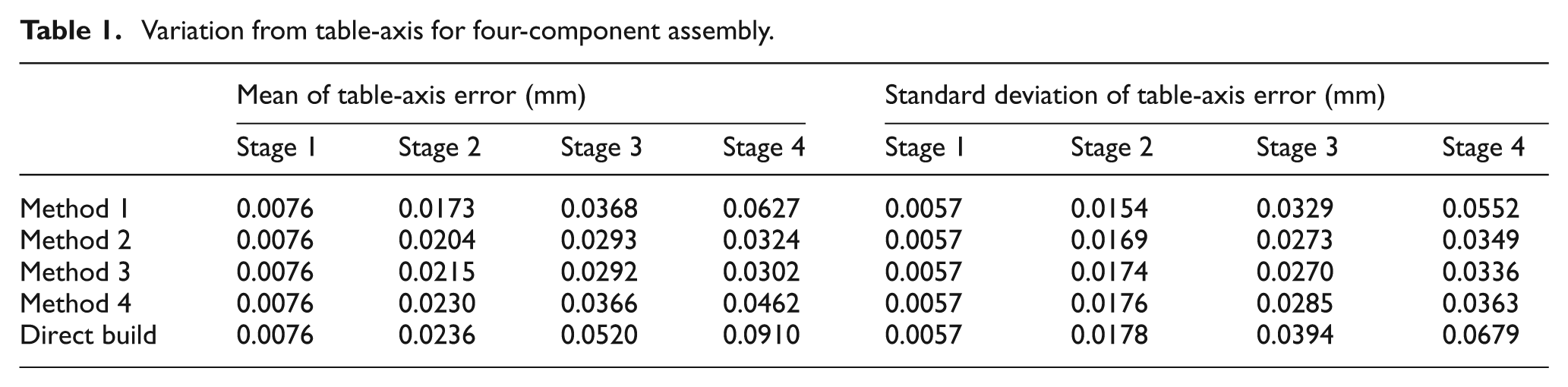
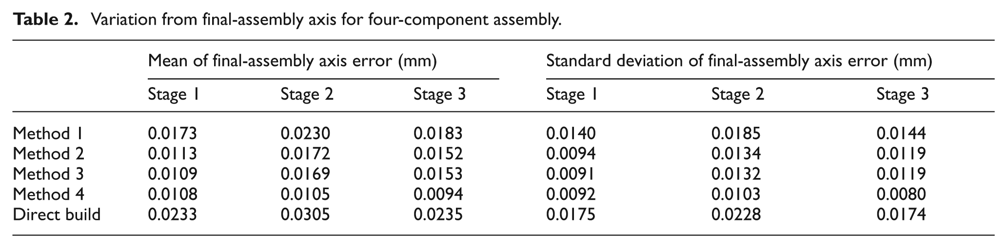
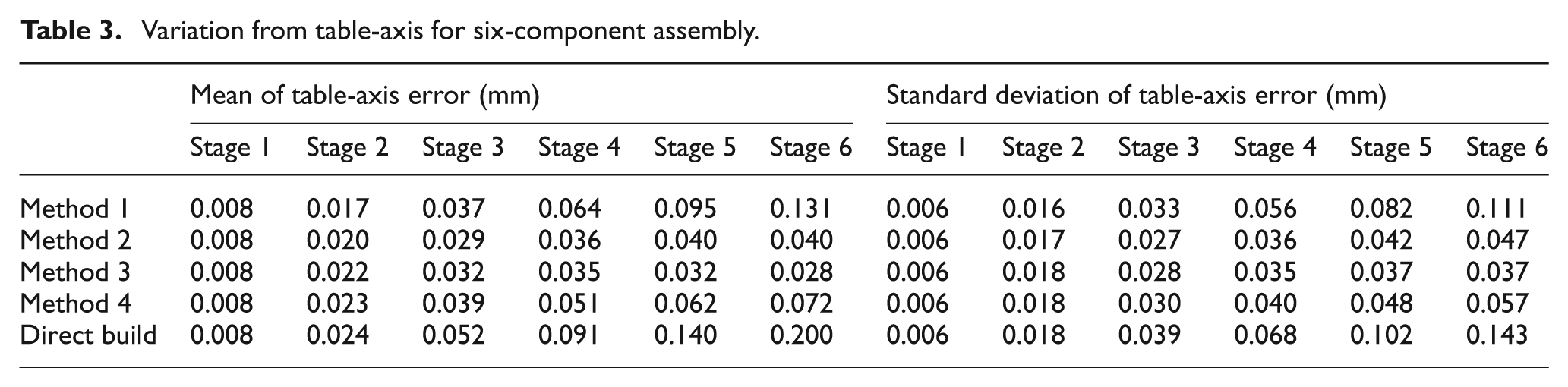
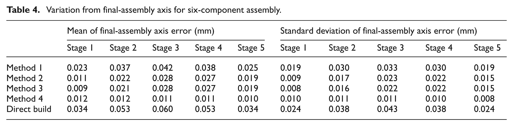
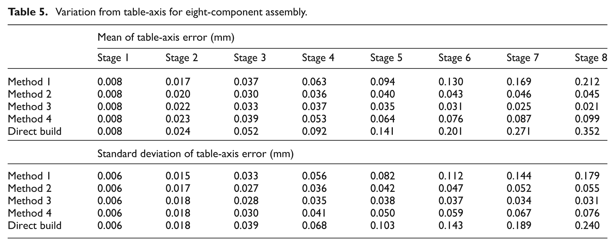
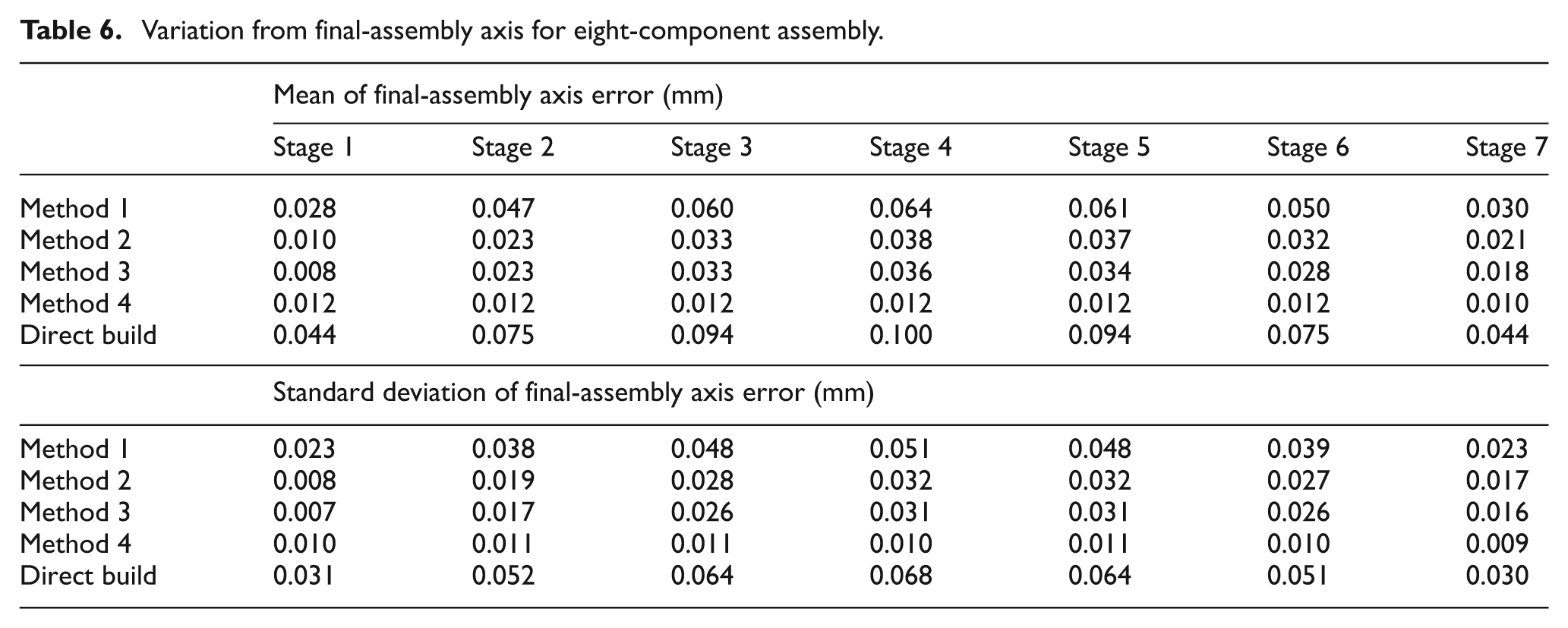
Figures 7–9 present results for the mean variation from the table-axis and final-assembly axis for the complete assembly (i.e. mean value of equation (23)) based on 50,000 repeated assemblies using the proposed optimisation methods and direct-build assembly, for 4, 6, and 8 component assemblies, respectively. Also, Tables 1, 3, and 5 present numerical results for the mean and standard deviations of table-axis error for the top of the upper-most component at each assembly stage, for 4, 6, and 8 component assemblies, respectively. Tables 2, 4, and 6 present numerical results for the mean and standard deviations of final-assembly axis error for the top of the upper-most component at each assembly stage, for 4, 6, and 8 component assemblies, respectively. In all cases it can be seen that all four optimisation methods yield assembly variations that are smaller than those obtained using direct-build assembly.

Figure 7.

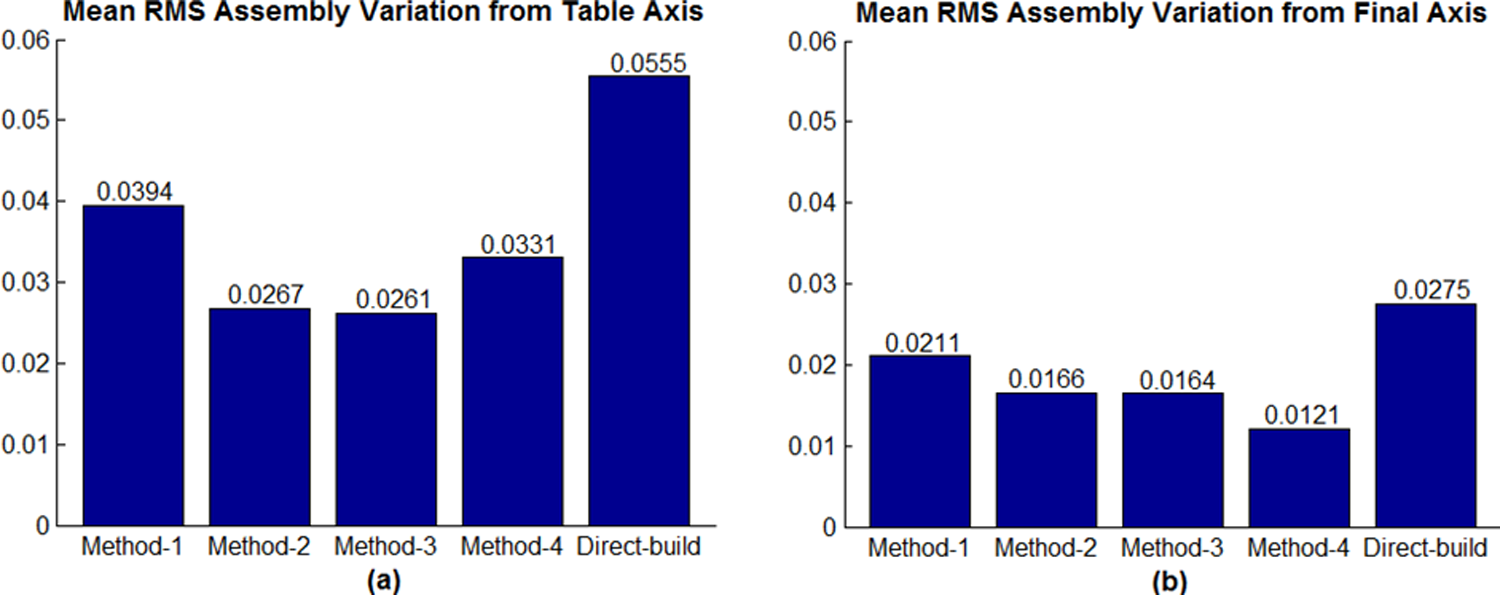
Mean of RMS assembly variation (equation (23)) based on 50,000 repeated assemblies for four-component assembly: (a) table-axis variation; (b) final-axis variation.

Figure 8.

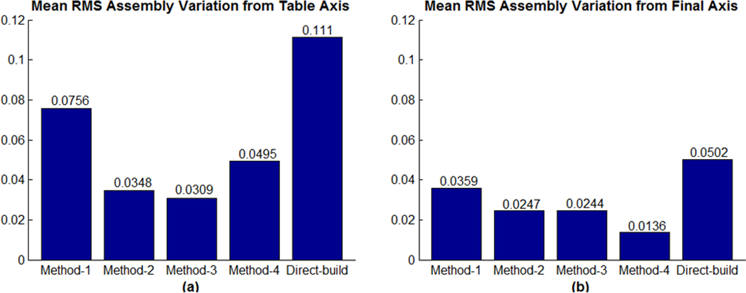
Mean of RMS assembly variation (equation (23)) based on 50,000 repeated assemblies for six-component assembly: (a) table-axis variation; (b) final-axis variation.

Figure 9.

Mean of RMS assembly variation (equation (23)) based on 50,000 repeated assemblies for eight-component assembly: (a) table-axis variation; (b) final-axis variation.

Table 1.

Variation from table-axis for four-component assembly.

	Mean of table-axis error (mm)				Standard deviation of table-axis error (mm)
	Stage 1	Stage 2	Stage 3	Stage 4	Stage 1	Stage 2	Stage 3	Stage 4
Method 1	0.0076	0.0173	0.0368	0.0627	0.0057	0.0154	0.0329	0.0552
Method 2	0.0076	0.0204	0.0293	0.0324	0.0057	0.0169	0.0273	0.0349
Method 3	0.0076	0.0215	0.0292	0.0302	0.0057	0.0174	0.0270	0.0336
Method 4	0.0076	0.0230	0.0366	0.0462	0.0057	0.0176	0.0285	0.0363
Direct build	0.0076	0.0236	0.0520	0.0910	0.0057	0.0178	0.0394	0.0679

Table 2.

Variation from final-assembly axis for four-component assembly.

	Mean of final-assembly axis error (mm)			Standard deviation of final-assembly axis error (mm)
	Stage 1	Stage 2	Stage 3	Stage 1	Stage 2	Stage 3
Method 1	0.0173	0.0230	0.0183	0.0140	0.0185	0.0144
Method 2	0.0113	0.0172	0.0152	0.0094	0.0134	0.0119
Method 3	0.0109	0.0169	0.0153	0.0091	0.0132	0.0119
Method 4	0.0108	0.0105	0.0094	0.0092	0.0103	0.0080
Direct build	0.0233	0.0305	0.0235	0.0175	0.0228	0.0174

Table 3.

Variation from table-axis for six-component assembly.

	Mean of table-axis error (mm)						Standard deviation of table-axis error (mm)
	Stage 1	Stage 2	Stage 3	Stage 4	Stage 5	Stage 6	Stage 1	Stage 2	Stage 3	Stage 4	Stage 5	Stage 6
Method 1	0.008	0.017	0.037	0.064	0.095	0.131	0.006	0.016	0.033	0.056	0.082	0.111
Method 2	0.008	0.020	0.029	0.036	0.040	0.040	0.006	0.017	0.027	0.036	0.042	0.047
Method 3	0.008	0.022	0.032	0.035	0.032	0.028	0.006	0.018	0.028	0.035	0.037	0.037
Method 4	0.008	0.023	0.039	0.051	0.062	0.072	0.006	0.018	0.030	0.040	0.048	0.057
Direct build	0.008	0.024	0.052	0.091	0.140	0.200	0.006	0.018	0.039	0.068	0.102	0.143

Table 4.

Variation from final-assembly axis for six-component assembly.

	Mean of final-assembly axis error (mm)					Standard deviation of final-assembly axis error (mm)
	Stage 1	Stage 2	Stage 3	Stage 4	Stage 5	Stage 1	Stage 2	Stage 3	Stage 4	Stage 5
Method 1	0.023	0.037	0.042	0.038	0.025	0.019	0.030	0.033	0.030	0.019
Method 2	0.011	0.022	0.028	0.027	0.019	0.009	0.017	0.023	0.022	0.015
Method 3	0.009	0.021	0.028	0.027	0.019	0.008	0.016	0.022	0.022	0.015
Method 4	0.012	0.012	0.011	0.011	0.010	0.010	0.011	0.011	0.010	0.008
Direct build	0.034	0.053	0.060	0.053	0.034	0.024	0.038	0.043	0.038	0.024

Table 5.

Variation from table-axis for eight-component assembly.

	Mean of table-axis error (mm)
	Stage 1	Stage 2	Stage 3	Stage 4	Stage 5	Stage 6	Stage 7	Stage 8
Method 1	0.008	0.017	0.037	0.063	0.094	0.130	0.169	0.212
Method 2	0.008	0.020	0.030	0.036	0.040	0.043	0.046	0.045
Method 3	0.008	0.022	0.033	0.037	0.035	0.031	0.025	0.021
Method 4	0.008	0.023	0.039	0.053	0.064	0.076	0.087	0.099
Direct build	0.008	0.024	0.052	0.092	0.141	0.201	0.271	0.352
	Standard deviation of table-axis error (mm)
Method 1	0.006	0.015	0.033	0.056	0.082	0.112	0.144	0.179
Method 2	0.006	0.017	0.027	0.036	0.042	0.047	0.052	0.055
Method 3	0.006	0.018	0.028	0.035	0.038	0.037	0.034	0.031
Method 4	0.006	0.018	0.030	0.041	0.050	0.059	0.067	0.076
Direct build	0.006	0.018	0.039	0.068	0.103	0.143	0.189	0.240

Table 6.

Variation from final-assembly axis for eight-component assembly.

	Mean of final-assembly axis error (mm)
	Stage 1	Stage 2	Stage 3	Stage 4	Stage 5	Stage 6	Stage 7
Method 1	0.028	0.047	0.060	0.064	0.061	0.050	0.030
Method 2	0.010	0.023	0.033	0.038	0.037	0.032	0.021
Method 3	0.008	0.023	0.033	0.036	0.034	0.028	0.018
Method 4	0.012	0.012	0.012	0.012	0.012	0.012	0.010
Direct build	0.044	0.075	0.094	0.100	0.094	0.075	0.044
	Standard deviation of final-assembly axis error (mm)
Method 1	0.023	0.038	0.048	0.051	0.048	0.039	0.023
Method 2	0.008	0.019	0.028	0.032	0.032	0.027	0.017
Method 3	0.007	0.017	0.026	0.031	0.031	0.026	0.016
Method 4	0.010	0.011	0.011	0.010	0.011	0.010	0.009
Direct build	0.031	0.052	0.064	0.068	0.064	0.051	0.030

Comparing all results for methods 1, 2, and 3 it can be seen that method 2 produces assemblies with smaller variations than method 1, and method 3 produces assemblies with smaller variations than method 2 (and method 1) for the different assemblies considered. This is not surprising because methods 1, 2, and 3 use increasingly sophisticated approaches to select the optimal configuration. Method 1 is a ‘local’ method based only on the errors for the component being considered. Method 2 considers errors in two components at a time, meaning that it makes some allowances for errors in subsequent stages of assembly. Finally, method 3 is a fully ‘global’ approach that considers all assembly stages simultaneously. It is also interesting to note that, for all cases considered, the variations obtained using method 2 are only slightly larger than those obtained using method 3. For an assembly with two components, methods 2 and 3 are equivalent, and this suggests these methods will yield similar results for components with a small number of components. However, the results shown indicate that this trend applies as the number of components is increased.

Method 4 consistently produces the smallest variation from the final-assembly axis for the different number of components. This is expected, because this optimisation method is based on minimising the final-assembly axis variation.

As the number of components increases, the proposed optimisation methods reduce assembly variation more significantly, compared with direct-build assembly. For example, from Figure 7, methods 1 and 2 reduce the variation by 29.2% and 50.3%, respectively, for the 4-component assembly; while for the 6-component assembly from Figure 8, methods 1 and 2 reduce the variation by 32.3% and 68.2%, respectively; for the 8-components assembly from Figure 9, methods 1 and 2 reduce the variation by 36.2% and 77.4%, respectively. These results indicate that the proposed optimisation methods are effective for any number of components in an assembly.

The above findings can be confirmed by considering the probability that the table or final-axis error for the final component in the assembly exceeds certain threshold values. The analysis performed to assess this probability is similar for assemblies with different numbers of components, and the findings are also similar. For this reason, only the results obtained for the 4 component assembly are presented here. The threshold values from the table-axis considered are: 0.05 mm, 0.1 mm, 0.15 mm, and 0.2 mm. Results for the probabilities that these threshold variations are exceeded are shown in Figure 10(a), where it can be seen that all optimisation methods are more effective than direct-build assembly. In addition, method 3 is superior to method 2, and method 2 is superior to method 1. Figure 10(b) shows results for the probability that the assembly variation from the final axis assembly exceeds 0.02 mm, 0.04 mm, 0.06 mm, and 0.08 mm. These results indicate that method 4 is more effective at reducing variation from final-axis than all other methods, as expected. However, it should be noticed that methods 3 and 4 are based on a combinatorial approach, which is potentially much less efficient than methods 1 and 2 in terms of computation time, particularly as the numbers of components and configurations increase. It also is difficult for the combinatorial approaches to be implemented, owing to the required added complexity. In practice, methods 1 and 2 have the potential to control the propagation of component variation, since they are easily implemented and have been shown to yield significant improvements compared with direct-build assembly, as described above. Furthermore, in all cases considered, the results obtained using method 2 are close to those obtained using the combinatorial approach (method 3), as shown in Figures 7, 8, and 9.

Figure 10.

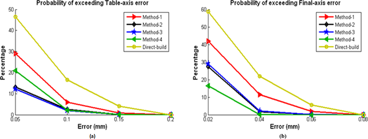
(a) Probability of the table-axis error exceeding 0.05 mm, 0.1 mm, 0.15 mm, and 0.2 mm, (b) probability of the final-axis error exceeding 0.02 mm, 0.04 mm, 0.06 mm, and 0.08 mm, for four identical component assemblies.

Example 2: non-identical components assembly

The dimensions of the components considered in example 2 are provided in Table 7 and represent scaled versions of components forming part of an aero-engine assembly used in industry. For this example, the tolerances used for the axial and radial run-outs in each component are 0.1 mm and 0.05 mm, respectively.

Table 7.

Dimensions of four components of the assembly.

Component	1	2	3	4
Height (H) (mm)	9	202	32	390
Width (B) (mm)	206	572	572	310

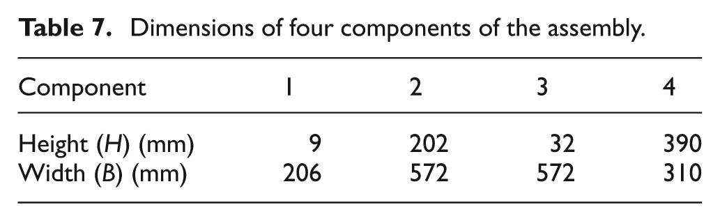
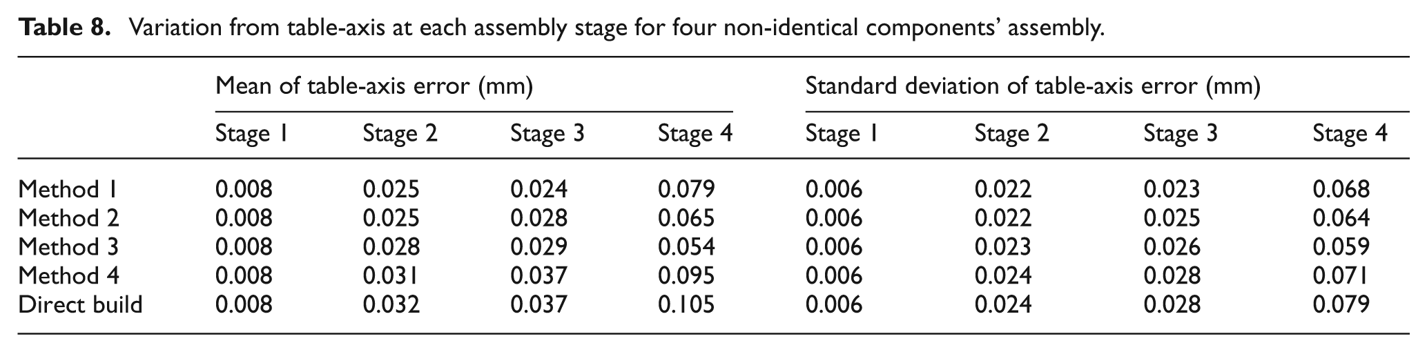
Figure 11 presents results for the mean assembly variation from the table-axis and final-assembly axis. These were obtained using 50,000 simulations in conjunction with the proposed optimisation methods and direct-build assembly. Similarly, Tables 8 and 9 present numerical results for the mean and standard deviations of table-axis error and final-assembly axis error for each assembly stage.

Figure 11.

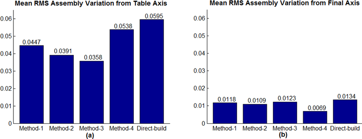
(a) Assembly variations from table-axis. (b) Assembly variations from final-assembly axis.

Table 8.

Variation from table-axis at each assembly stage for four non-identical components’ assembly.

	Mean of table-axis error (mm)				Standard deviation of table-axis error (mm)
	Stage 1	Stage 2	Stage 3	Stage 4	Stage 1	Stage 2	Stage 3	Stage 4
Method 1	0.008	0.025	0.024	0.079	0.006	0.022	0.023	0.068
Method 2	0.008	0.025	0.028	0.065	0.006	0.022	0.025	0.064
Method 3	0.008	0.028	0.029	0.054	0.006	0.023	0.026	0.059
Method 4	0.008	0.031	0.037	0.095	0.006	0.024	0.028	0.071
Direct build	0.008	0.032	0.037	0.105	0.006	0.024	0.028	0.079

Table 9.

Variation from final-assembly axis for four non-identical components’ assembly.

	Mean of final-assembly axis error (mm)			Standard deviation of final-assembly axis error (mm)
	Stage 1	Stage 2	Stage 3	Stage 1	Stage 2	Stage 3
Method 1	0.008	0.012	0.013	0.006	0.009	0.010
Method 2	0.008	0.010	0.011	0.006	0.008	0.009
Method 3	0.008	0.013	0.012	0.006	0.010	0.010
Method 4	0.007	0.005	0.005	0.006	0.004	0.005
Direct build	0.008	0.014	0.014	0.006	0.010	0.011

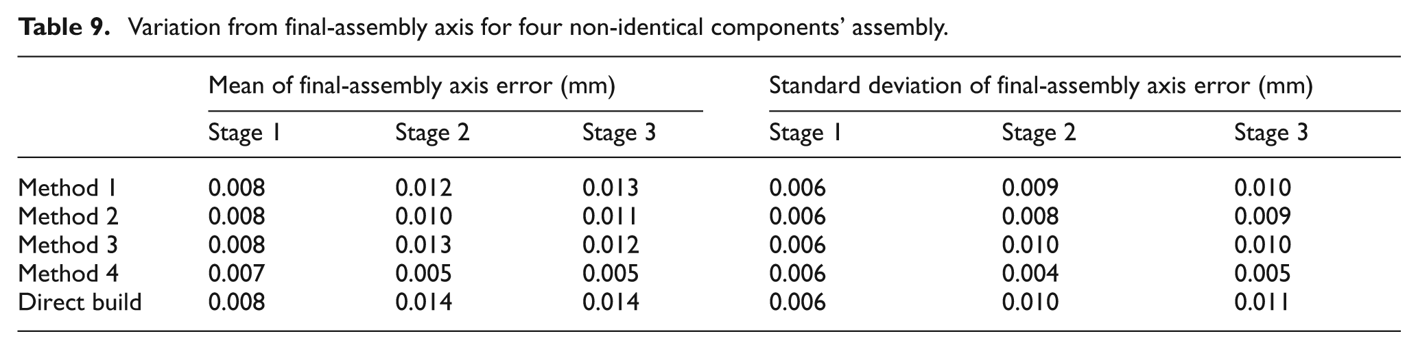
In all cases the four optimisation methods produce lower variations than direct-build assembly. From Tables 8 and 9, it is found that the standard deviation of the variation increases with stage for all methods for both table-axis and final axis measures. Comparing all of these results, identical trends to those indicated for example 1 are found, with method 3 producing the smallest variation from the table-axis and method 4 producing the smallest variation from the final-assembly axis. Further, confirmation of these findings is presented in Figure 12, which plots the probability that the assembly variation from the table-axis and final-assembly axis exceed particular values.

Figure 12.

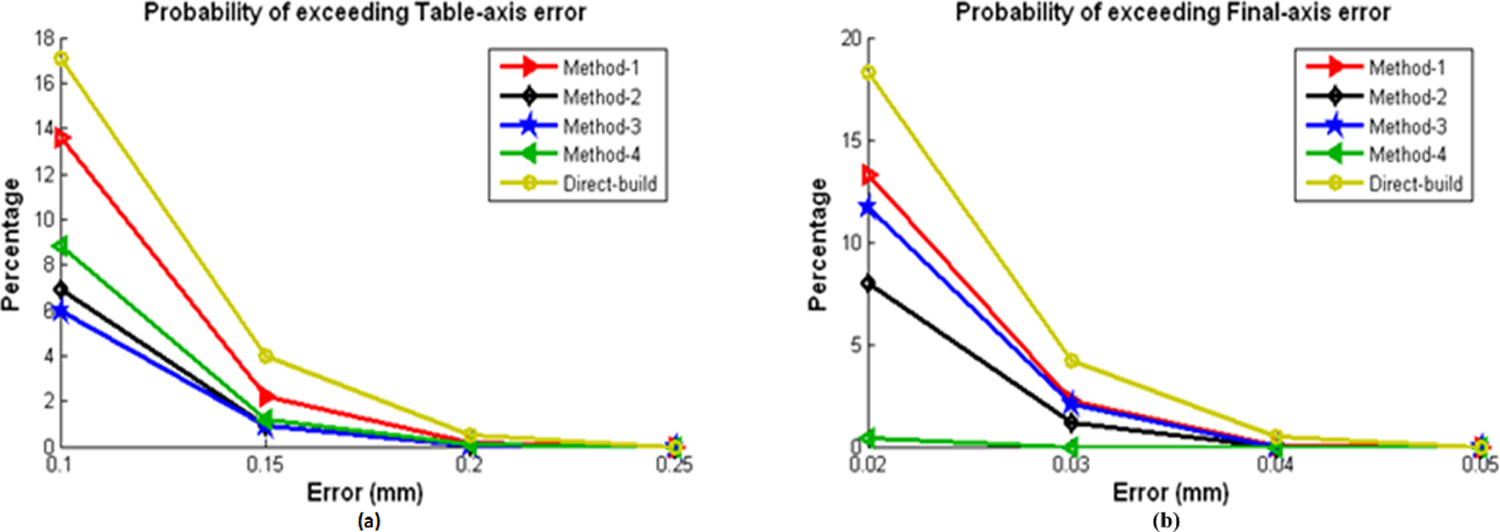
(a) Probability of the table-axis error exceeding 0.1 mm, 0.15 mm, 0.2 mm, and 0.25 mm. (b) Probability of the final-axis error exceeding 0.02 mm, 0.03 mm, 0.4 mm, and 0.5 mm.

In summary, the proposed optimisation methods have demonstrated good potential to reduce variation propagation in axi-symmetric mechanical assemblies. Although methods 3 and 4 produce the smallest variations, it is important to realise that these methods are based on a combinatorial approach, which is potentially much less efficient than the other proposed methods, particularly as the number of components increases. For example, for a N-component assembly, the total number of combinations of the complete assembly to be computed is $2^{N-1}$ . In addition to this, it is unlikely that combinatorial approaches would be implemented in practice, owing to the required added complexity. Despite this, the results presented for these methods are useful because they provide the best possible outcome, which is useful for comparison when considering the performance of the other methods.

It is clear from the examples considered that methods 1 and 2 have the potential to control the propagation of component variation, and significant improvements to assembly variations are possible compared with direct-build assembly – in all of the cases considered the results obtained using method 2 are reasonably close to those obtained using the combinatorial approach (method 3). However, any potential improvements are likely to depend on the geometry and complexity of the mechanical assembly being considered.

Summary

This article uses connective assembly models to calculate variation propagation in the assembly of axi-symmetric components. The variations considered for each component are expressed in terms of the radial and axial run-outs (following ISO standards^26,35) and have been treated as a source of translation and rotation error in the mating features for each component in the assembly. Novel optimisation techniques for straight-build assembly have been proposed, which use relative orientation techniques to reduce assembly variation by selecting the optimal orientation of neighbouring components. The optimisation methods considered are based on:

• stage-by-stage optimisation (method 1);

• two consecutive stage optimisation (method 2);

• combinatorial approaches (methods 3 and 4). Methods 1–3 minimise the table-axis eccentricity error, while method 4 minimises eccentricity from the final-assembly axis.

Monte Carlo simulations have been used to investigate the statistical performance of each method for two assembly examples.

The results presented indicate that all proposed optimisation methods produce significantly improved eccentricities compared with direct-build (without optimisation). The combinatorial approaches (methods 3 and 4) are fully ‘global’ and consider all assembly stages simultaneously, and always yield the smallest possible eccentricities. However, practical complexities, including potentially large numbers of calculations, make them unsuitable for practical implementation currently. Although, methods 1 and 2 are not as effective as method 3 for reducing table-axis variations, they have been shown to produce good improvements compared with direct-build, with method 2 always producing smaller eccentricities than method 1. This can be explained by noting that method 1 is a ‘local’ method based only on component errors for the component being assembled, while method 2 simultaneously considers errors in two components, meaning that it makes some allowances for errors in subsequent stages of assembly. For the examples considered it was found that method 2 was only slightly less effective that method 3 in reducing assembly variation, and all methods continue to be effective as the number of components is increased.