Sage Journals: Discover world-class research

Abstract

Many automobile companies are actively exploring the use of high-strength dual-phase steels as an alternative to aluminum and magnesium alloys owing to their light weight, low cost and durability. However, dual-phase steels have a tendency to springback more than other structural steels in a forming operation owing to their high tensile strength. In addition, variations in manufacturing process parameters and material properties cause springback variation over different manufactured parts. Therefore, it is an important task to reduce the magnitude of springback, as well as its variation within, to produce robust and cost-effective parts. This article investigates minimization of the magnitude and variation of springback of DP600 steels in U-channel forming within a robust optimization framework. The computational cost was reduced by utilizing metamodels for prediction of the springback and its variation during optimization. Three different allowable sheet thinning levels were considered in solving the robust optimization problem, and it was found that, as the allowable thinning increased, the die radius decreased, thereby the magnitude and variation of springback reduced. A simple sensitivity analysis was performed and the yield stress was found to be the most important random variable. Finally, a double-loop Monte Carlo simulation method was proposed to calculate part-to-part and batch-to-batch springback variations. It was found that, as the batch-to-batch variation of yield stress increased, the batch-to-batch springback variation increased, while the part-to-part springback variation remained unchanged.

Keywords

Robust optimization springback dual-phase steels Monte Carlo simulations metamodels

Introduction

Springback can be defined as the deviation of the manufactured geometry from the designed geometry, and it is one of the most important problems observed during the sheet metal forming process. The high strength of dual-phase steels leads to more springback than those of the traditional steels. Moreover, variations of the manufacturing process parameters and material properties lead to springback variation over different manufactured parts. Reducing the variation of springback is as important as reducing the magnitude of springback, because it limits the application of springback prediction and compensation techniques.^1,2 Therefore, it is an important task to reduce the magnitude of springback, as well as its variation within, to produce robust and cost-effective parts.

There are numerous studies in literature that only focus on the reduction of the magnitude of springback. Gomes et al.³ and Zhang and Lee⁴ showed that an efficient springback magnitude reduction can be achieved by first determining the most influential process parameters, and then performing the required actions. Liu⁵ introduced the effect of a restraining force on shape deviation to minimize the springback. Karafillis and Boyce⁶ developed a methodology for tool and binder design based on inverse springback calculations. This proposed method gives rapid results for simple geometries, but complex geometries may require long-term iterations. Even though these studies provide insights, they did not consider springback variation. However, accurate determination of the uncertainties in material properties and forming process parameters provides more reliable results and improves the final product quality, hence a robust optimization study is required.

Hilditch et al.⁷ investigated the effect of yielding behavior on side wall curl and springback of DP600 and transformation induced plasticity (TRIP) steels. They examined the effect of back tension and strain aging. Wang et al.⁸ performed experimental and numerical studies in order to investigate the effect of tooling parameters on the anticlastic curvature that occurred during the sheet metal forming operations. They observed that increase, both in the tension and tool radius, decreases the amount of springback, however, a larger tool radius has less significant effect. Carden et al.⁹ investigated the effect of friction coefficient and ratio of die radius to sheet thickness (R/t) on the springback behavior for high-strength low alloy (HSLA), deep-quality special killed (DQSK) steels and 6022 T4 aluminum alloy. They showed that friction has a minor effect on springback, contrary to some other literature studies, such as Hino et al.¹⁰ However, a very low coefficient of friction results in an increasing amount of springback for aluminum. They also observed that increasing R/t ratio decreases the springback.

A robust optimization study is conducted to achieve maximum average performance with minimum variation in the presence of uncontrollable uncertainties. In literature, there exists simulation based,^11,12 as well as experimental¹³ robust optimization studies. Robust optimization requires performing uncertainty analysis¹⁴ and Monte Carlo simulations (MCS) are usually performed for that purpose.¹⁵

The aim of robust springback optimization is to obtain minimum average springback with minimum variation. Wang et al.² investigated a systematic and robust approach, gathering the finite element method (FEM) and stochastic statistics to decrease the sensitivity of high-strength steels (HSS) stamping in the presence of uncertainties. A study by de Souza and Rolfe¹⁶ examined a probabilistic analytical model, where the variation of five input parameters and their relationship to the springback were investigated. Zhang and Shivpuri¹⁷ studied the reliability of optimum variable blank holder force (BHF) in the presence of process uncertainties by minimizing the magnitude of wrinkling and fracture defects under probabilistic constraints. Mullerschon et al.¹⁸ considered the uncertainties in the manufacturing processes of metal forming to estimate the random variations with the aid of finite element simulations. Lönn et al.¹⁹ presented an alternative approach to robust optimization, where the robustness of each design was examined through multiple sampling of the stochastic variables at each design point. Du et al.²⁰ studied the robustness and robust mechanism synthesis when random and interval variables are involved. Harlow²¹ investigated the effect of variability in material properties on springback, where only within-batch variability is considered. In addition, no variability, other than the variability in material properties, was considered in that study. Similarly, Gantar and Kuzman²² presented an approach that integrated the response surface methodology and MCSs. The latest, and most comprehensive, study on this subject was proposed by Chen and Koç,¹ which analyzed the effect of material properties and some process parameters (sheet thickness, BHF and friction coefficient) variation on springback. All these mentioned studies have considered only part-to-part or within-batch variations while leaving the batch-to-batch variation out of analysis owing to the difficulty of traveling batch-to-batch variability with part-to-part and within-batch variability in a same loop. However, Majeske and Hammett²³ showed that batch-to-batch variations cannot be neglected at all. The main contribution of this article is that the batch-to-batch and part-to-part springback variation is traveled simultaneously using a double-loop strategy.

In this article, robust optimization of U-channel forming is performed by considering the three different sheet thinning levels. Then, the double loop is performed to calculate the part-to-part and batch-to-batch springback variations.

Springback analysis

The FEM is the most popular method for springback calculation. A fine mesh grid, right element type and size are required for a proper implementation of the FEM. At the same time, contact definition, solution algorithm and convergence criterion have crucial effects on the results.^24–27 The FEM is widely used when the problem is complex,^28–32 however, since the FEM is time consuming, its direct integration to a robust-optimization study is computationally prohibitive.

For simple problems, as in the case of this study, analytical methods are preferred for both their computational advantage and easy coupling to a robust optimization study. In this article, an analytical model proposed by Dongjuan et al.³³ is used to predict the sheet springback of U-channel forming (Figure 1). This model is based on Hill48 yielding criterion³⁴ and a plane strain condition, and takes the effects of sheet thinning and thickness, hardening coefficient, blank holding force, coefficient of friction and anisotropy into account.

Figure 1.

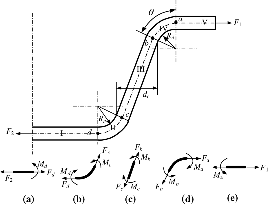
The free body diagram in the U-channel sheet forming process. Source: reprinted with permission from Elsevier.³³

The following assumptions are applied by Dongjuan et al.³³ in the sheet stretch-bending process (Figure 2).

Figure 2.

The strain distribution in sheet stretch-bending,³³ where L_n is the length of neutral surface and L_m is the arc length of sheet middle surface. Source: reprinted with permission from Elsevier.³³

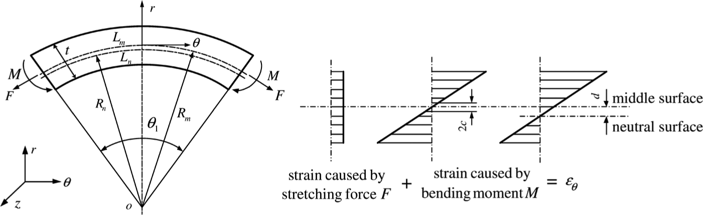
F (the stretching force per unit width) is assumed to remain constant throughout the thickness. It leads to sheet thinning.

Straight lines and neutral surface are orthogonal during the stretch–bending process.

ϵ_z is zero while the thickness/width ratio is small.

Volume is constant during the stretch–bending process.

The following formula gives the amount of final sheet thickness at the end of U-channel forming process

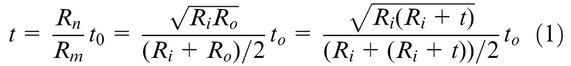
t = \frac{R_{n}}{R_{m}} t_{0} = \frac{\sqrt{R_{i} R_{o}}}{(R_{i} + R_{o}) / 2} t_{o} = \frac{\sqrt{R_{i} (R_{i} + t)}}{(R_{i} + (R_{i} + t)) / 2} t_{o}

(1)

where t is the final sheet thickness in mm and R_i is the die radius in mm. The following formulas can be used to determine the bending radius of the outer surface (i.e. R_o), middle surface (i.e. R_m), and neutral surface (i.e. R_n), respectively.

R_{o} = R_{i} + t

(2)

R_{n} = \sqrt{R_{i} R_{o}}

(3)

R_{m} = (R_{i} + R_{o}) / 2

(4)

The anisotropy coefficient (f) can be formulated as

f = \frac{1 + R}{\sqrt{1 + 2 R}}

(5)

where R is the normal isotropy.

The half thickness of the elastic region (c) is

c = \frac{f {\bar{σ}}_{s} R_{n}}{E_{1}}

(6)

E_{1} = \frac{E}{1 - ν^{2}}

(7)

where ${\bar{σ}}_{s}$ is the yield stress, E is the modulus of elasticity and E₁ is the modulus of elasticity under plane strain conditions. Elastic deformation can be observed at the region of ±c distance away from the middle surface. $σ_{m θ}$ is equal to the stress caused by stretching force F

σ_{m θ} = fk {(ε_{0} + f \ln \frac{R_{m}}{R_{n}})}^{n} R_{n} + c \leq R_{m} \leq R_{0}

(8)

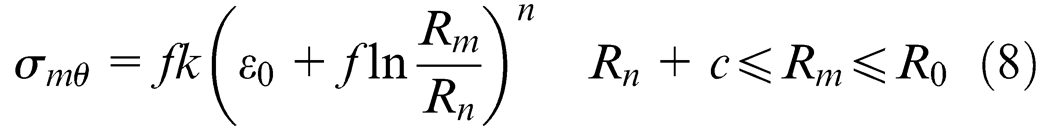
where k is the hardening coefficient and n is the hardening exponent. The bending moment (M) can be calculated as

M = b \int_{R_{m} - t / 2}^{R_{n} - c} {- fk {[ε_{0} - f \ln (\frac{r}{R_{n}})]}^{n} - σ_{m θ}} (r - R_{m}) dr + b \int_{R_{n} - c}^{R_{n} + c} (\frac{E}{1 - ν^{2}} \ln (\frac{r}{R_{n}}) - σ_{m θ}) (r - R_{m}) dr + b \int_{R_{n} + c}^{R_{m} + t / 2} {fk {[ε_{0} + f \ln (\frac{r}{R_{n}})]}^{n} - σ_{m θ}} (r - R_{m}) dr

(9)

During the reverse bending process the change of bending moment ( $Δ M$ ) can be formulated as

Δ M = \int_{R_{n} + c}^{R_{o}} {- fk {[ε_{0} + f \ln (\frac{r}{R_{n}}) - 2 {\bar{ε}}_{lim}]}^{n} - f {\bar{σ}}_{s} - σ'_{m θ}} (r - R_{m}) dr + \int_{R_{i}}^{R_{n} - c} [fk {(ε_{0} - f \ln (\frac{r}{R_{n}}) - 2 {\bar{ε}}_{lim})}^{n} + {\bar{σ}}_{s} - σ'_{m θ})] (r - R_{m}) dr + \int_{R_{n} - c}^{R_{n} + c} [- E_{1} (\frac{r - R_{n}}{R_{n}}) - σ'_{m θ}] (r - R_{m}) dr

(10)

In the U-channel forming process, the blank is subjected to cyclic loading. Therefore, Bauschinger’s effect³⁵ should be taken into consideration. For this purpose, the stress state during unloading was described using the kinematic hardening model.³⁶ $σ'_{θ}$ is the tangential stress after unloading

| {σ'}_{θ} | = {\begin{matrix} E_{1} | \ln \frac{r}{R_{n}} | & R_{n} - c \leq r \leq R_{n} + c \\ fk {(ε_{0} + | f \ln \frac{r}{R_{n}} | - 2 {\bar{ε}}_{lim})}^{n} + f {\bar{σ}}_{s} & R_{i} \leq r \leq R_{n} - c or R_{n} + c \leq r \leq R_{o} \end{matrix}

(11)

$σ'_{m θ}$ is the stress in the sheet middle surface after reverse stretch bending

σ'_{m θ} = σ_{m θ} - fk {[ε_{0} + f \ln (\frac{r}{R_{n}}) - 2 {\bar{ε}}_{lim}]}^{n} - f {\bar{σ}}_{s}

(12)

After the bending moment is calculated, the springback can be calculated from

\begin{matrix} Δ θ = \int_{0}^{θ} \frac{M (ϕ)}{E_{1} I} R_{n} d ϕ; M (ϕ) = M + Δ M \end{matrix}

(13)

\begin{matrix} Δ θ_{sw} = \frac{M_{b} L}{E_{1} I}; \end{matrix}

(14)

where Δθ is the angular change during springback regions II and IV, Δθ_sw is the angular change during springback in region III, (I = t³/12) is the inertia moment of the cross-section per unit width, M_b is defined in Fig. 1(c) and L is length of sidewall. Therefore, the acute angle of the final geometry can be calculated as

θ = 90^{0} + Δ θ - (Δ θ_{sw} / 2)

(15)

The difference between the desired bending angle and the final angle is

Δ θ_{sb} = 90^{\circ} - θ

(16)

where Δθ_sb is the springback value.

Definition of the robust optimization problem

For this simple problem, there is a single design variable: the die radius, R_d. The robust optimization problem can be formulated as

find R_{d}

(17a)

min . w_{1} \frac{μ_{Δ θ} (R_{d})}{μ_{Δ θ} (R_{d} = {(R_{d})}_{nom})} + w_{2} \frac{σ_{Δ θ} (R_{d})}{σ_{Δ θ} (R_{d} = {(R_{d})}_{nom})}

(17b)

s . t . Pr [\frac{Δ t (R_{d})}{t_{0}} \leq \frac{Δ t_{spec}}{t_{0}}] \geq 0.99

(17c)

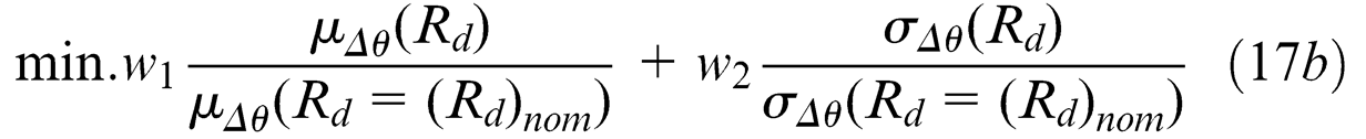
In equation (17), both the mean and the standard deviation of springback (µ_Δ _θ and σ_Δ _θ ) were minimized. The weighting factors w₁ and w₂ were chosen based on the importance of reducing the mean and the standard deviation of springback and also satisfy w₁ + w₂ = 1. For example, if minimizing the mean value of springback is more important than minimizing the standard deviation, the weighting factors are selected as w₁ > w₂. (R_d)_nom is the nominal value for die radii. Depending on the sheet thinning constraint, the value of (R_d)_nom was taken as 0.85, 0.54 and 0.37, corresponding to 5%, 10% and 15% sheet thinning, respectively. Since the problem of interest was formulated in terms of a single design variable and sheet thinning, and springback values compute with each other in a U-channel stamping problem, the constraint in equation (17) was always active. In this case, the R_d value obtained from the constraint function became the solution of the robust optimization problem regardless of the value of the objective function.

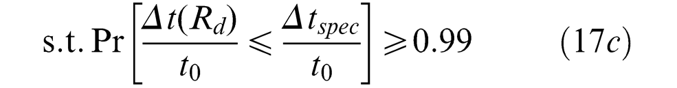
In this study, the reliability level was set to 99% for the probabilistic constraint (see equation 17c). This means that only a single profile out of 100 produced U-profiles was allowed to have a sheet thinning value above the prespecified allowable value. In this study, the allowable sheet thinning values of 5%, 10% and 15% were used, and the effect of this allowable value on the optimum solution was explored. The sheet thinning was assumed to follow the normal distribution. Hence, the R_d value that ensures the mentioned 99% reliability constraint can be obtained using equation (18). To calculate R_d, the mean and standard deviation values of sheet thinning (µ_Δ _t and σ_Δ _t ) depending on R_d must be known. In this study, metamodels were constructed to relate µ_Δ _t and σ_Δ _t values to R_d. After metamodels were constructed, the value of R_d, satisfying equation (17c), can easily be calculated. Note that in equation (18) the 99% reliability value corresponded to z = 2.326

\frac{\frac{μ_{Δ t} (R_{d})}{t_{0}} - \frac{Δ t_{spec}}{t_{0}}}{\frac{σ_{Δ t} (R_{d})}{t_{0}}} = z (z = 2.326 \Rightarrow ϕ (z) = 0.99)

(18)

Double-loop MCS to analyze part-to-part and batch-to-batch springback variation

In this study, springback variation was classified into two components: part-to-part and batch-to-batch variation. Part-to-part variation is the variability of a property (e.g. sheet thickness) between different parts that are produced using the same material batch. The batch-to-batch variation, on the other hand, represents the variability of a property between different material batches.

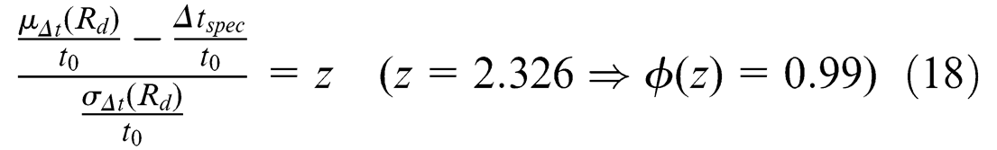
Consider the U-channel stamping operation performed by a company. The company obtains the batches of sheet metals from N_b different manufacturers. The characteristic material properties, as well as geometric properties for each batch, may change from one to that of another. Similarly, for sheet metals from a specified manufacturer (that is, for a specific batch), N_p number of parts are assumed to be produced. For a specific batch, the material or geometric properties may change from a produced part to another. To observe the effect of these changes on springback, the use of a double-loop MCS is proposed that considers different batches and different parts. The double-loop MCS code was composed of two loops, where the inner loop simulates N_p number of different parts and the outer loop simulates N_b number of different batches (Figure 3). Overall, a total sample of size N_b × N_p was generated and batch-to-batch and part-to-part springback variation were computed.

Figure 3.

Double-loop MCS model.

For the problem of interest, there exists five random variables to be considered: (a) σ_Y, yield stress, (b) K, hardening coefficient, (c) R, normal anisotropy, (d) n, hardening exponent, and (e) t, sheet thickness. To simplify the analysis in the double-loop MCS, first the most influential random variable was determined, and then the effect of the batch-to-batch and part-to-part variation of the most influential variable on the batch-to-batch and part-to-part variation of the springback was explored. This was achieved by assigning variability to the standard deviation of the most influential variable as discussed in the next sections.

Results and discussions

In this section, first the robust optimization problem defined in equation (17) was solved for three different allowable sheet thinning values. The effects of the allowable sheet thinning value on the optimization results were explored. Next, the deterministic variant of equation (17) was solved and the results were compared with those of the robust optimization. The advantages of robust optimization over deterministic optimization were investigated. Then, a simple sensitivity analysis was performed to determine the most influential random variable. This information can be very useful for a company manager to decide how to allocate the company resources on reducing uncertainties. Finally, the double loop MCS strategy was applied to the problem of interest, and part-to-part and batch-to-batch springback variations were evaluated owing to the part-to-part and batch-to-batch variation of the most influential variable.

Solution of the robust optimization problem for three different allowable sheet thinning levels

Determination of R_d value for 5% sheet thinning constrain

To determine the R_d value that ensures 5% sheet thinning with 99% reliability, first metamodels were constructed for mean and standard deviation of sheet thinning in terms of R_d. To construct a metamodel, first an interval of R_d was determined and then MCS was performed to calculate mean and standard deviation values of springback and sheet thinning. Finally, metamodels were constructed between R_d values with obtained mean and standard deviation values. As shown in Table 1, seven R_d values were chosen within the range 0.7–1.0 mm, and mean and standard deviation values of springback and sheet thinning were calculated by the MCS. After the metamodels were constructed, the R_d value leading to 5% sheet thinning and the corresponding springback values can easily be assessed.

Table 1.

MCS (10,000 samples) results for R_d values within the range 0.7–1.0 mm.

No.	R_d (mm)	Springback (°)			Sheet thinning (%)
		Avg	Std	CV	Avg	Std	CV
1	0.7	2.326	0.105	0.045	6.278	0.080	0.013
2	0.75	2.349	0.108	0.046	5.759	0.075	0.013
3	0.8	2.362	0.111	0.047	5.304	0.070	0.013
4	0.85	2.383	0.112	0.047	4.899	0.067	0.014
5	0.9	2.404	0.115	0.048	4.539	0.063	0.014
6	0.95	2.422	0.118	0.049	4.218	0.060	0.014
7	1	2.448	0.120	0.049	3.930	0.056	0.014

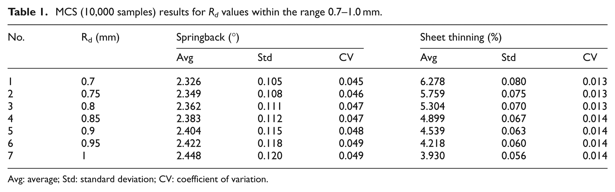
Avg: average; Std: standard deviation; CV: coefficient of variation.

Several different types of metamodels exist in literature; polynomial response surface,^37–39 radial-basis functions (RBFs),³⁹ Kriging,^40–41 artificial neural networks,^42–43 etc. For brief descriptions of these metamodels, the reader should refer to Acar and Rais-Rohani⁴⁴ and Acar et al.⁴⁵ For the data in Table 1, a second-order polynomial response surface (PRS2), RBFs and Kriging (zeroth-order trend model, KR0 and first-order trend model, KR1) metamodel types were constructed. Accuracy of the constructed metamodels was evaluated by using leave-one-out cross-validation errors computed at the data points. To compute the leave-one-out cross-validation error, metamodels were constructed N times (where N is the number of data points), each time leaving out one of the data points. The difference between the exact response at the omitted point and that predicted by each variant metamodel defines the cross-validation error. After this procedure was applied to all data points, the root mean square error (RMSE), mean absolute error (MAE) and maximum absolute error (MAXE) of cross-validation errors were calculated and the results listed in Tables 2 and 3.

Table 2.

Accuracy evaluation via the cross-validation error of metamodels constructed for mean and standard deviation values of springback.

Metamodel type	Mean value of springback			Standard deviation of springback
	RMSE	MAE	MAXE	RMSE	MAE	MAXE
PRS2	0.0024	0.0017	0.0048	0.0003	0.0003	0.0006
RBF	0.0053	0.0035	0.0105	0.0048	0.0032	0.0088
KR0	0.0046	0.0027	0.0115	0.0013	0.0010	0.0029
KR1	0.0031	0.0024	0.0060	0.0002	0.0002	0.0005

Bold font represents the smallest error metric.

RMSE: root mean square error; MAE: mean absolute error; MAXE: maximum absolute error.

Table 3.

Accuracy evaluation via the cross-validation error of metamodels constructed for mean and standard deviation values of sheet thinning.

Metamodel type	Mean value of sheet thinning			Standard deviation of sheet thinning
	RMSE	MAE	MAXE	RMSE	MAE	MAXE
PRS2	0.0175	0.0140	0.0313	0.0003	0.0002	0.0005
RBF	0.0138	0.0092	0.0257	0.0037	0.0025	0.0068
KR0	0.0139	0.0093	0.0294	0.0013	0.0011	0.0011
KR1	0.0186	0.0126	0.0388	0.0008	0.0006	0.0017

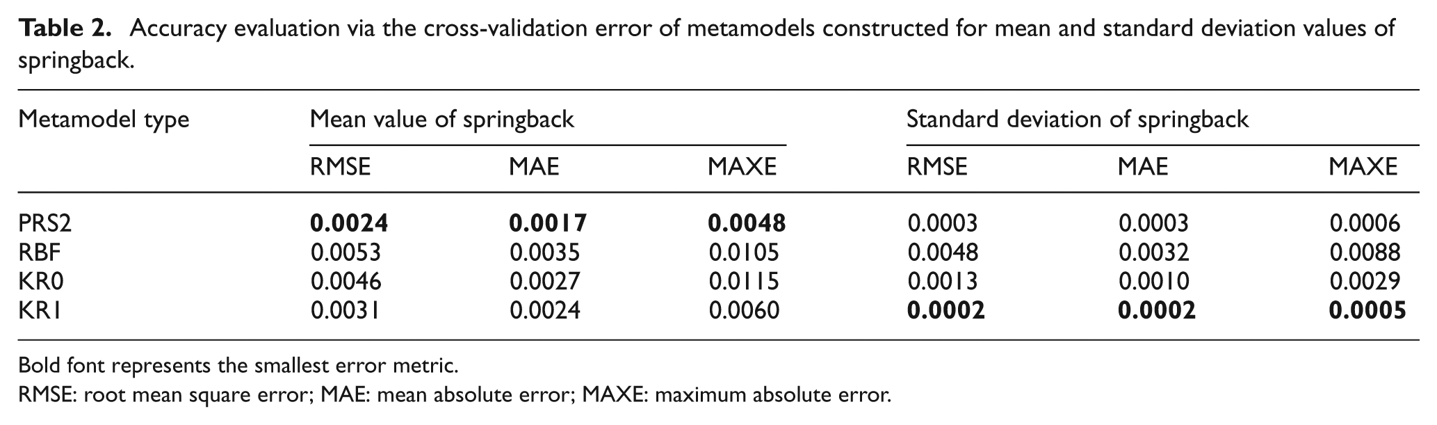
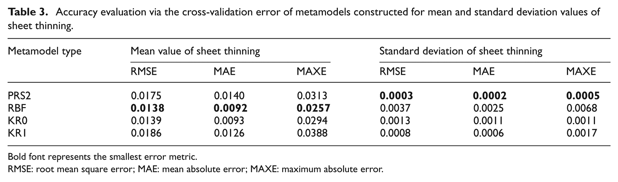
Bold font represents the smallest error metric.

RMSE: root mean square error; MAE: mean absolute error; MAXE: maximum absolute error.

Accuracy evaluation of constructed metamodels for the mean and standard deviation of springback was presented in Table 2. PRS2 was found to be the most accurate metamodel type for the mean value of springback, and KR1 for its standard deviation. For standard deviation, the second most accurate model was found to be PRS2. Both construction and interpretation (mathematical expression is easier and straightforward) of PRS2 models are easier than the other metamodel types. Hence, PRS2 was used for both mean and standard deviation values of springback. The constructed metamodels were found to be accurate when the error metrics presented in Table 2 were compared with the values presented in Table 1. The constructed PRS2 models were shown in Figure 4(a) and (b), and their mathematical formulation is given in Appendix 2. The high R² values also confirmed the accuracy of PRS2.

Figure 4.

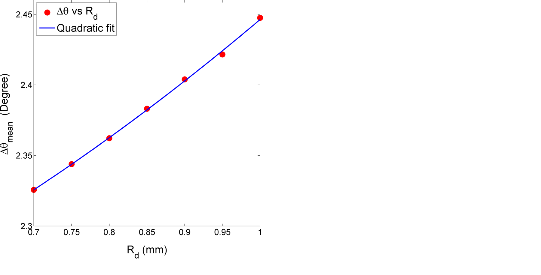
The metamodel constructed for (a) the mean value, and (b) the standard deviation of springback in terms of the die radius between 0.7 mm and 1.0 mm.

Accuracy of constructed metamodels for mean and standard deviation values of sheet thinning are given in Table 3. The RBF was found to be the most accurate metamodel type for the mean value of sheet thinning, and PRS2 for its standard deviation. The third most accurate model was PRS2 among the four constructed metamodel types for standard deviation. As noted earlier, both creation and interpretation of PRS2 models are easier than the other metamodel types. Hence, PRS2 was decided to be used for both mean and standard deviation values of sheet thinning. In addition, constructed metamodels were found to be considerably accurate when error metrics presented in Table 3 are compared with the presented values in Table 1. The constructed PRS2 models were presented in Figures 5(a) and (b). The high R² values (see Appendix 2) also indicate the high accuracy of PRS2.

Figure 5.

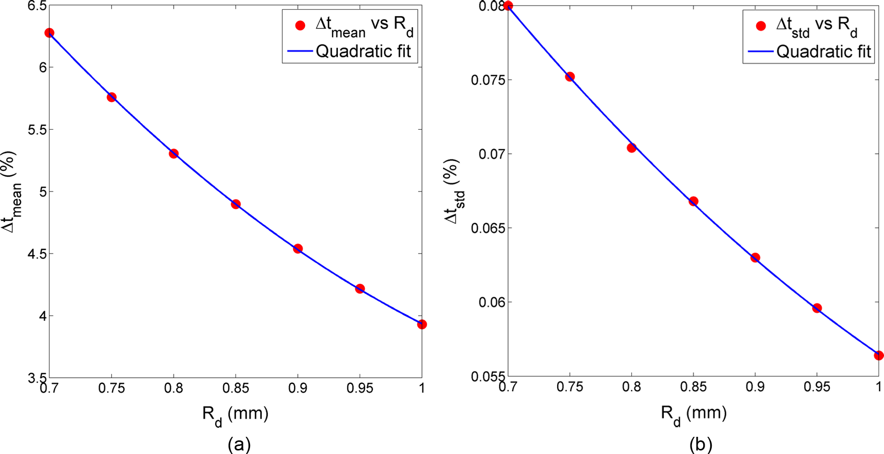
The metamodel constructed for (a) the mean value, and (b) the standard deviation of sheet thinning in terms of the die radius between 0.7 mm and 1.0 mm.

In Figure 5(a) and (b), the equations of constructed PRS2 metamodels are also shown. These PRS2 equations were used in the robust optimization constraint equation (that is, equation (18)). The optimum R_d value was calculated as 0.96 mm, which ensured the 5% sheet thinning value with 99% reliability. For this calculated radius value, the mean value of sheet thinning was calculated as approximately 4.15%. When the MCS (with 10,000 samples) was performed for R_d = 0.96 mm, the mean value of sheet thinning was calculated approximately as 4.16%. It was another indication that the results obtained from the PRS2 were quite accurate.

Determination of R_d value for 10% sheet thinning constraint

Similar to study for 5% sheet thinning, new PRS2 models were constructed to determine R_d, which ensured the 10% sheet thinning value safely. Seven different values were determined for die radius R_d within the range 0.48–0.6 mm. With the guidance of the study for 5% sheet thinning, PRS2 models were constructed for all responses. The constructed PRS models are given in Appendix 2. The graphical depictions of the PRS models were not provided owing to space limitations.

The optimum R_d value was calculated as 0.56 mm, which ensured the 10% sheet thinning value with 99% reliability. For this calculated radius value, the mean value of sheet thinning was calculated as approximately 8.18%. When the MCS (with 10,000 samples) was performed for R_d = 0.56 mm, the mean value of sheet thinning was calculated as approximately 8.18%. It showed that the results obtained from PRS2 were quite accurate.

Determination of R_d value for 15% sheet thinning constraint

Next, new PRS2 models were constructed to determine R_d, which ensures the 15% sheet thinning value safely. Seven different values were determined for die radius R_d within the range 0.31–0.43 mm. Once again, PRS2 models were constructed for all responses. The constructed models were given in Appendix 2. The graphical depictions of the PRS models were not provided once more owing to space limitations.

The optimum R_d value that ensured the 15% sheet thinning value with 99% reliability was calculated as 0.38 mm. For this calculated radius value, the mean value of sheet thinning was calculated as approximately 12.27%. When the MCS (with 10,000 samples) is performed for R_d = 0.38 mm, the mean value of sheet thinning was calculated as approximately 12.28%.

Table 4 shows the optimization results for three different allowable thinning levels. It is seen from Table 4 that, as the allowable thinning level increases, the optimum die radii reduces, thereby the magnitude as well as the variation of the springback decreases. Notice that the variation was represented by using the coefficient of variation, which is the standard deviation over the mean value.

Table 4.

The change of die radii, as well as the magnitude and variation of springback and sheet thinning, with respect to the allowable thinning level.

Allowable thinning level (%)	Die radii (mm)	Springback (°)		Sheet thinning (%)
		Mean	COV	Mean	COV
5	0.96	2.427	0.049	4.160	0.014
10	0.56	2.282	0.043	8.177	0.012
15	0.38	2.250	0.040	12.282	0.010

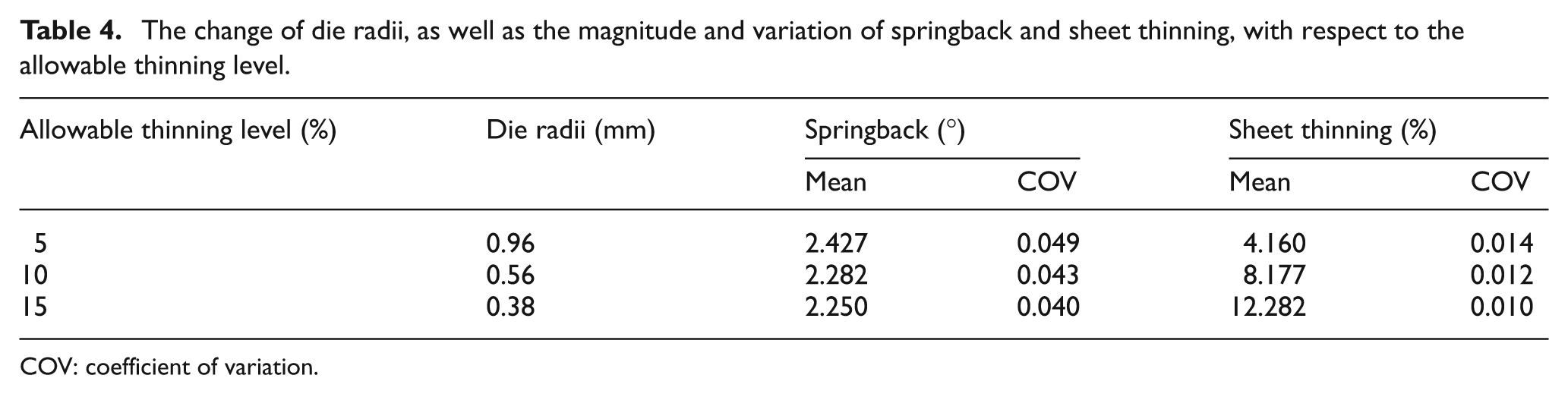
COV: coefficient of variation.

Comparison of the results of deterministic and robust optimization

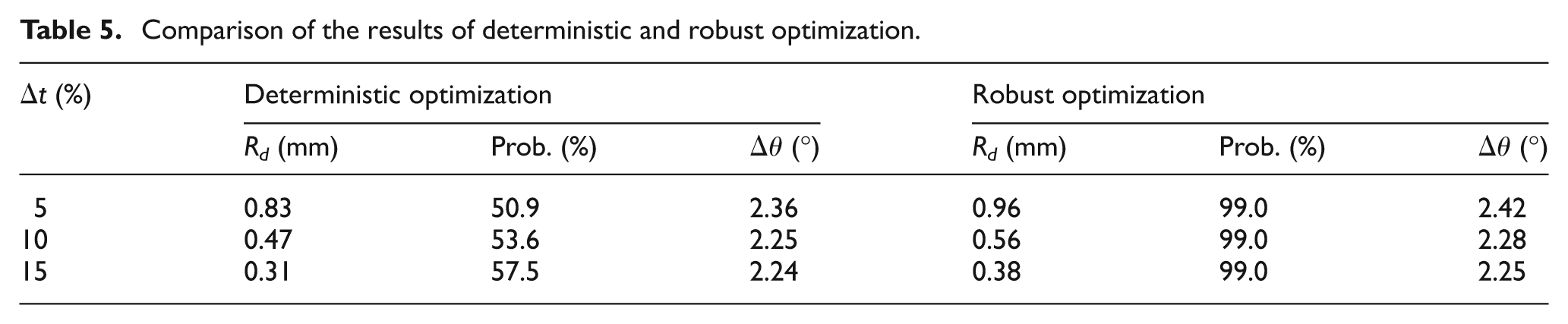
To emphasize the advantages of robust optimization over deterministic optimization, a deterministic variant of equation (17) was solved, where all the random variables took their mean values. The comparison of the results of robust optimization to those of the deterministic optimization was presented in Table 5. It was seen that the reliability of sheet thinning being smaller than the allowable value was around 50% (as expected). It means that there is about a 50% chance that the sheet thinning value will be smaller than the allowable value. For the case of robust optimization, on the other hand, the reliability of sheet thinning being smaller than the allowable value is 99% (a pre-specified value). The robust optimum R_d values were found to be larger than the deterministic optimum R_d values. Therefore, the springback values corresponding to the robust optimum were slightly larger than those of the deterministic optimum. That is, to maintain the reliability of sheet thinning being smaller than a certain value, it was required to settle for slightly larger springback values.

Table 5.

Comparison of the results of deterministic and robust optimization.

Δt (%)	Deterministic optimization			Robust optimization
	R_d (mm)	Prob. (%)	Δθ (°)	R_d (mm)	Prob. (%)	Δθ (°)
5	0.83	50.9	2.36	0.96	99.0	2.42
10	0.47	53.6	2.25	0.56	99.0	2.28
15	0.31	57.5	2.24	0.38	99.0	2.25

The sensitivity analysis to determine the most influential random variable

A simple sensitivity analysis was performed to determine the most influential random variable. The influence of each random variable was evaluated through the following procedure.

The value of the random variable of interest was set to µ-3σ and µ + 3σ, respectively, while keeping the other random variables at their mean values.

The springback values corresponding to these two settings were calculated.

The difference between the springback values is a measure of the influence of that random variable.

For each variable, µ-3σ and µ + 3σ values are provided in Table 6.

Table 6.

µ -3σ and µ + 3σ values of random variables.

	µ-3σ	µ	µ + 3σ
σ_Y (MPa)	295.87	389.30	482.73
K (MPa)	1023.76	1060.49	1097.23
R	1.03	1.135	1.24
n	0.2004	0.2054	0.2104
t (mm)	0.77	0.8	0.83

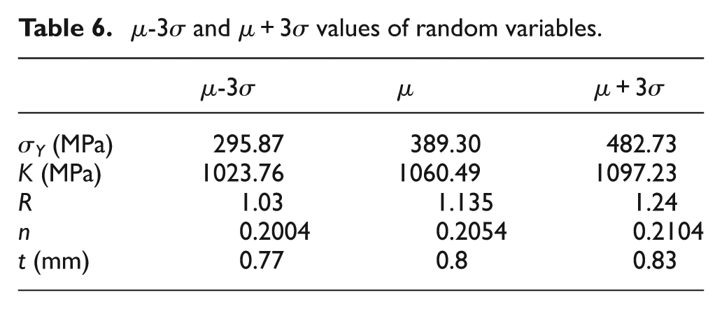
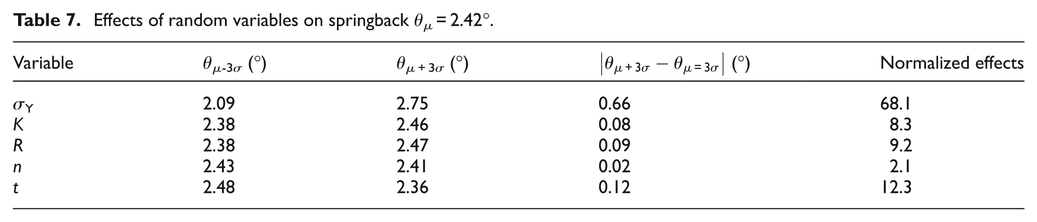
The computed springback results are listed in Table 7. When all the random variables take their mean values, the springback was calculated as θ_µ = 2.42°. The second column in Table 7 shows the springback results when the random variable of interest takes its own µ-3σ value and the others take their mean values. For example, when yield stress was σ_Y = µ-3σ = 295.87 MPa and the other random variables take their mean values, springback was calculated as θ = 2.09°. Similarly, the third column in Table 7 shows the springback results when a random variable of interest takes the value of µ + 3σ while the other random variables take their mean values. The fourth column in Table 7 shows the difference between second and third columns. The fifth column shows the normalized values of the fourth column. As seen from the fifth column in Table 7, the yield stress was found to be the most influential random variable.

Table 7.

Effects of random variables on springback θ_µ = 2.42°.

Variable	θ_µ-3σ (°)	θ_{µ + 3σ} (°)	$\| θ_{μ + 3 σ} - θ_{μ = 3 σ} \|$ (°)	Normalized effects
σ_Y	2.09	2.75	0.66	68.1
K	2.38	2.46	0.08	8.3
R	2.38	2.47	0.09	9.2
n	2.43	2.41	0.02	2.1
t	2.48	2.36	0.12	12.3

Application of double loop MCS

A robust springback optimization study requires calculation of the springback variation, and this variation can be divided into three categories.²³

Part-to-part variation.

Within-batch variation.

Batch-to-batch variation.

The part-to-part variation is the amount of variation between parts produced in the same production process. The within-batch variation is the amount of variation between parts produced from the same batch. The batch-to-batch variation represents the variability from one batch to another.

In this section, the simulation of batch-to-batch variability of the most influential random variable σ_Y is explained. It maybe assumed that the mean values of the yield stress for all batches are the same and equal to the target value specified by the company. So the mean value (µ) of σ_Y was set to σ_Y = µ> = 389.3 MPa for every supplier. However, the standard deviation (σ) of yield stress for each batch is taken to be different for each supplier as each material supplier may have a different quality control practice. The standard deviation of yield stress was assumed to be uniformly distributed among different suppliers. The lower and the upper bound for the standard deviation of the yield stress was computed from $σ_{b}^{L} = {\bar{σ}}_{b} - b_{b}$ and $σ_{b}^{U} = {\bar{σ}}_{b} + b_{b}$ , respectively, where b_b is named as the bound-of-batch value. To explore the effect of batch-to-batch variation, six different bounds of batch values (b_b) were considered, as listed in Table 8.

Table 8.

Distribution parameters for part-to-part and batch-to-batch variations.

Part-to-part		Batch-to-batch
µ	σ	$μ_{σ_{b}}$	(b_b)₁	(b_b)₂	(b_b)₃	(b_b)₄	(b_b)₅	(b_b)₆
389.3	31.1	31.1	0	5	10	15	20	25

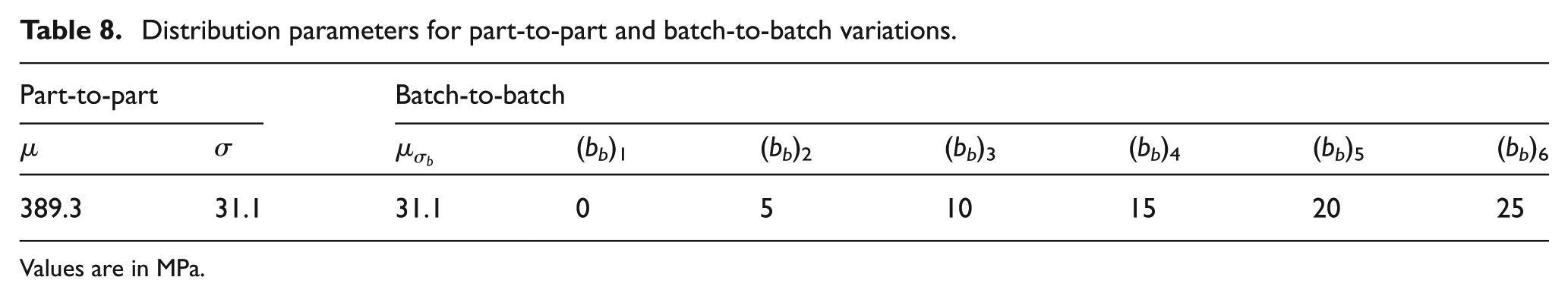
Values are in MPa.

Part-to-part and batch-to-batch springback variation evaluation

To examine the part-to-part and batch-to-batch springback variation, the following method was applied to a 100 × 100 matrix (size of parts × size of batches), which contains the springback results obtained from the MCS. To determine the part-to-part variation, first the standard deviations of each column was calculated $(σ_{p_{i}})$ , and then the mean value of standard deviations of all columns was calculated $(mean (σ_{p_{i}}))$ . This calculated value is equal to part-to-part variation. To determine batch-to-batch variation, first the standard deviations of each row was calculated $(σ_{b_{i}})$ , then the mean value of the standard deviations of all rows was calculated $(mean (σ_{b_{i}}))$ . This calculated value is equal to the batch-to-batch variation.

Each column has a different standard deviation of yield stress. This standard deviation was drawn from a uniform distribution using the specific bound-of-batch and mean values. So, standard deviation of yield stress changes from its lower bound to upper bound progressing from left to right in the 100 × 100 matrix. Also, each row represents a different yield stress value. From the first to last row, random numbers were drawn from the normal distribution. From top to bottom, the cumulative distribution function was changed from zero to one to draw the random values. To assign real values to the yield stress, the cumulative distribution function (CDF) value was taken as 10⁻⁴ instead of 0, and 1–10⁻⁴ instead of 1. Therefore, the columns of the 100 × 100 matrix represent different batches, while the rows of the matrix represent different parts.

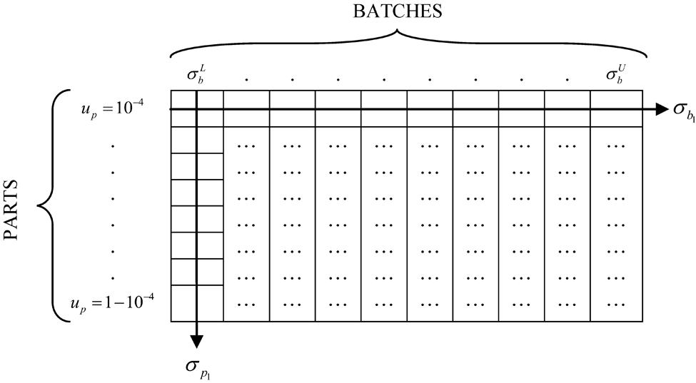
As shown in Figure 6, the batch-to-batch variation can be found by calculating the mean value of each row’s standard deviation value $(mean (σ_{b_{1}}, σ_{b_{2}}, σ_{b_{3}} \dots σ_{b_{N_{b}}}))$ . Similarly, the part-to-part variation can be determined by calculating the mean value of each column’s standard deviation value $(mean (σ_{p_{1}}, σ_{p_{2}}, σ_{p_{3}} \dots σ_{p_{N_{p}}}))$ . Note that for a fixed yield stress value, the calculation of standard deviation between columns gives the batch-to-batch springback behavior. Similarly, for a fixed standard deviation value of yield stress the calculation of standard deviation between rows gives the part-to-part springback behavior.

Figure 6.

Determination of the batch-to-batch and part-to-part variation from the 100 × 100 matrix.

The results obtained from the double-loop analysis are depicted in Figure 7. It was seen that if the bound-of-batch value of yield stress increases, the ratio of batch-to-batch springback variation to part-to-part variation increases as expected.

Figure 7.

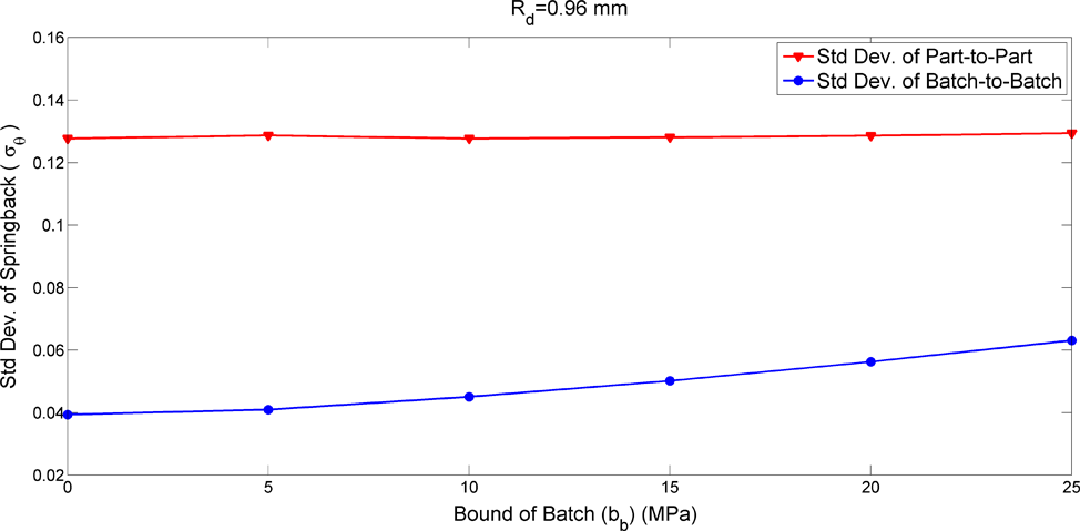
The variation of standard deviation of springback with respect to the bound-of-batch of the yield stress for R_d = 0.96 mm.

Conclusion

In this study, the magnitude, as well as the variation the springback of U-profile sheets made of DP600 dual phase steels, were minimized using a robust optimization methodology. An analytical model was used to predict the sheet springback. The robust optimization problem was formulated to minimize the mean and the standard deviation of springback subject to a probabilistic constraint on sheet thinning. The mean and the standard deviation values of springback, as well as sheet thinning, were computed through MCSs. To reduce the computational burden, metamodels were constructed for the prediction of mean and standard deviation of springback as well as sheet thinning. From the obtained results, the following conclusions were drawn:

Four different types of metamodels were utilized, namely PRS2, RBF and Kriging (KR0 and KR1). PRS2 was found to be the most accurate metamodel type for mean value of springback and its standard deviation.

Three different sheet thinning levels were considered and it is found that as the allowable thinning level increases, the optimum die radius (R_d) value decreases, thereby the magnitude and variation of springback reduces.

In addition, the deterministic variant of the robust optimization problem was also solved. The robust optimum R_d values were found to be larger than the deterministic optimum R_d values. Therefore, the springback values corresponding to the robust optimum were obtained slightly larger than those of the deterministic optimum. That is, maintaining the reliability of sheet thinning to be smaller than a certain value leads to slightly increased springback values.

A simple sensitivity analysis was performed to determine the most influential random variable and yield stress was found to be the most influential random variable. This information can be very useful for a company manager to decide how to allocate the company resources on reducing uncertainties. For this problem, it was more effective to allocate the resources for tighter quality control measures that can reduce the uncertainty in yield stress.

A double-loop MCS methodology was proposed to simulate the effects of different material batches and different parts. The batch-to-batch and part-to-part springback variation values were computed. It was found that, as the batch-to-batch variability of yield stress increased, the batch-to-batch springback variation increased, while the part-to-part springback variation remained unchanged.

Note that a simple geometry and analytical model is used in this study. The geometry is based on a benchmark problem of NUMISHEET’93.⁴⁶ The hardening model is based on Hill48 yielding criterion. Therefore, most of the results are mainly applicable for the analyzed problem. For instance, it was found that the yield stress was the most influential parameter. If a different material model or a different yielding criterion is used, a different parameter might be found as the most important parameter. Similarly, a PRS2 was found to be the most accurate metamodel type for the mean and standard deviation of the springback. For different geometry and loading/boundary conditions, a different metamodel type might be found as the most accurate metamodel type. These issues can be the subject of further studies.

Footnotes

Appendix 1

Appendix 2 Funding

This research is supported by TÜBİTAK (The Scientific and Technological Research Council of Turkey), under award MAG 109M078.

References

Chen

Koç

. Simulation of springback variation in forming of advanced high strength steels. J Mater Process Technol 2007; 190: 189–198.

Wang

Hou

Lin

. An engineering approach to improve the stamping robustness of high strength steels. J Mfg Sci E-T 2009; 131: ASME 064501.

Gomes

Onipede

Lovell

. Investigation of springback in high strength anisotropic steels. J Mater Process Technol 2005; 159: 91–98.

Zhang

Lee

. Effects of process variables and material properties on the springback behavior of 2D-draw bending parts. SAE paper 9500692, 1995.

Liu

. The effect of restraining force on shape deviation in flanged channels. J Eng Mater T ASME 1988; 110: 389–394.

Karafillis

Boyce

. Tooling and binder design for sheet metal forming processes compensating springback error. Int J Mach Tool Mf 1996; 36: 503–526.

Hilditch

Speer

Matlock

. Influence of low-strain deformation characteristics of high strength sheet on curl and springback in bend-under-tension tests. J Mater Process Technol 2007; 182: 84–94.

Wang

Wagoner

Matlock

. Antielastic curvature in draw-bend springback. Int J Solids and Structures 2005; 42: 1287–1307.

Carden

Geng

Matlock

. Measurement of springback. Int J Mech Sci 2002; 4(1): 79–101.

10.

Hino

Goto

Shirashi

. Springback of sheet metal laminates subjected to stretch bending and the subsequent unbending. Advd Technol Plasticity 1999; II: 1077–1082.

11.

Wang

Lee

. Robust design of finned-tube evaporators: a scalable product platform approach. Proc IMechE, Part B: J Engineering Manufacture 2009; 223(11): 1483–1495.

12.

. Robust design and analysis of 4PUS–1RPU parallel mechanism for a five-degree-of-freedom hybrid kinematics machine. Proc IMechE, Part B: J Engineering Manufacture 2011; 225(5): 685–698.

13.

Acar

Camuscu

. Experimental robust optimal machining of hardened AISI 420 stainless steel with Al₂O₃+TiCN mixed ceramic tool. Proc IMechE, Part B: J Engineering Manufacture 2011, 225(7): 1033–1039.

14.

Ahn

Hwang

Choi

. Error analysis of the cutting coefficients and optimization of calibration procedure for cutting force prediction. Proc IMechE, Part B: J Engineering Manufacture 2011, 225(2): 149–162.

15.

Yang

Hussain

Popov

. Novel optimization technique for variation propagation control in an aero-engine assembly. Proc IMechE, Part B: J Engineering Manufacture 2011; 225(1): 100–111.

16.

de Souza

Rolfe

. Multivariate modeling of variability in sheet metal forming. J Mater Process Technol 2008; 203(1–3): 1–12.

17.

Zhang

Shivpuri

. Investigating reliability of variable blank holder force control in sheet drawing under process uncertainties. J Mfg Sci E-T 2008; 130: ASME 041001.

18.

Mullerschon

Lorenz

Roll

. Reliability based design optimization with LS OPT for a metal forming application. LS DYNA Anwenderforum Frankenthal 2007; CIII: 1–14.

19.

Lönn

Fyllingen

Nilssona

. An approach to robust optimization of impact problems using random samples and meta modeling. Int J Impact Eng 2009; 37: 723–734.

20.

Venigella

Liu

. Robust mechanism synthesis with random and interval variables. Mech Mach Theory 2009; 44: 1321–1337.

21.

Harlow

. The effect of statistical variability in material properties on springback. Int J Mater and Prod Technol 2004; 20(1–3): 180–192.

22.

Gantar

Kuzman

. Optimization of stamping processes aiming at maximal process stability. J Mater Process Technol 2005; 167: 237–243.

23.

Majeske

Hammett

. Identifying sources of variation in sheet metal stamping. Int J Flex Mf Sys 2003; 15: 5–18.

24.

Shi

Prince

Song

. A sensitivity study of simulation parameters in sheet metal forming and springback simulation using LS-DYNA. In: Proceedings of the fifth international LS-DYNA users conference, vol.6, Southfield, MI, September, 1998, p. 6.

25.

Shi

Zhang

. Issues concerning material constitutive laws and parameters in springback simulations. SAE SP435, 1999.

26.

Lin

Liu

. Study on the effects of numerical parameters on the precision of springback prediction. In: Proceedings of the sixth international LS-DYNA users conference, Session 13.3, Detroit, MI, April, 2000, p. 5.

27.

. A few issues on accuracy of springback simulation of automobile parts. SAE SP 1435, 1999.

28.

Finn

Galbraith

Hallquist

. Use of a coupled explicit–implicit solver for calculating spring-back in automotive body panels. J Mater Process Technol 1995; 50(1–4): 395–409.

29.

Narasimhan

Lovell

. Predicting springback in sheet metal forming: an explicit to implicit sequential solution procedure. Finite Elem Analysis Des 1999; 33: 29–42.

30.

Leu

. Simplified approach for evaluating bend ability and springback in plastic bending of anisotropy sheet metals. J Mater Process Technol 1997; 66: 9–17.

31.

Pourboghrat

Chung

Richmond

. A hybrid membrane/shell method for rapid estimation of springback in anisotropy sheet metals. J Appl Mech T ASME 1998; 65(3): 671–684.

32.

Tan

Liew

. Springback analysis for sheet forming processes by explicit finite element method in conjunction with the orthogonal regression analysis. Int J Solids Struct 1999; 36: 4653–4668.

33.

Dongjuan

Zhenshan

Xueyu

. An analytical model for predicting springback and side wall curl of sheet after U-bending. Comp Mater Sci 2007; 38: 707–715

34.

Hill

. The mathematical theory of plasticity. London: Oxford University Press, 1950.

35.

Tang

Wang

. Springback investigation of anisotropic aluminum alloy sheet with a mixed hardening rule and Barlat yield criteria in sheet metal forming. Mater Design 2010; 31: 2043–2050.

36.

Ragai

Lazim

Nemes

. Anisotropy and springback in draw-bending of stainless steel 410: experimental and numerical study. J Mater Process Technol 2005; 166: 116–127.

37.

Myers

Montgomery

. Response surface methodology: process and product optimization using designed experiments. New York: Wiley, 1995.

38.

Box

GEP

Draper

. Response surfaces, mixtures, and ridge analyses. 2nd ed. New Jersey: Wiley, 2002.

39.

Buhmann

. Radial basis functions: theory and implementations. New York: Cambridge University Press, 2003.

40.

Sacks

Welch

Mitchell

. Design and analysis of computer experiments. Stat Sci 1989; 4(4): 409–435.

41.

Simpson

Mauery

Korte

. Kriging models for global approximation in simulation-based multidisciplinary design optimization. AIAA J 2001; 39: 12.

42.

Bishop

. Neural networks for pattern recognition. New York: Oxford University Press, 1995.

43.

Haykin

. Neural networks: a comprehensive foundation. 2nd ed. Ontario: Prentice Hall, 1998.

44.

Acar

Rais-Rohani

. Ensemble of metamodels with optimized weight factors. Struct Multidiscip O 2009; 37(3): 279–294.

45.

Acar

Guler

Gerçeker

. Multi-objective crashworthiness optimization of tapered thin-walled tubes with axisymmetric indentations. Thin Wall Struct 2011; 49(1): 94–105.

46.

NUMISHEET’93, In: Proceedings of the second international conference of numerical simulation of 3-D sheet metal forming processes, Isehara, Japan, 1993.

Analyzing batch-to-batch and part-to-part springback variation of DP600 steels using a double-loop Monte Carlo simulation

Abstract

Keywords

Introduction

Springback analysis

Definition of the robust optimization problem

Double-loop MCS to analyze part-to-part and batch-to-batch springback variation

Results and discussions

Solution of the robust optimization problem for three different allowable sheet thinning levels

Determination of Rd value for 5% sheet thinning constrain

Determination of Rd value for 10% sheet thinning constraint

Determination of Rd value for 15% sheet thinning constraint

Comparison of the results of deterministic and robust optimization

The sensitivity analysis to determine the most influential random variable

Application of double loop MCS

Part-to-part and batch-to-batch springback variation evaluation

Conclusion

Footnotes

Appendix 1

Appendix 2

Funding

References

Determination of R_d value for 5% sheet thinning constrain

Determination of R_d value for 10% sheet thinning constraint

Determination of R_d value for 15% sheet thinning constraint