
Abstract
Voting paradoxes date back to the origin of social choice theory in the 18th century, when the Chevalier de Borda pointed out that plurality—then and now the most common voting rule—may elect a candidate who loses pairwise majority comparisons against every other candidate. Since then, a large number of similar, seemingly paradoxical, phenomena have been observed in the literature. As it turns out, many paradoxes only materialize under some rather contrived circumstances and require a certain number of voters and candidates. In this paper, we leverage computational optimization techniques to identify the minimal numbers of voters and candidates that are required for the most common voting paradoxes to materialize. The resulting compilation of voting paradoxes may serve as a useful reference to social choice theorists as well as an argument for the deployment of certain rules when the numbers of voters or candidates are severely restricted.
Introduction
Electoral systems are a crucial pillar of liberal democracy. The formal properties of electoral systems are studied in social choice theory, whose origins can be traced back to the Age of Enlightenment, in particular during the French Revolution, and whose modern development was initiated by Arrow’s impossibility theorem. In its simplest form, the central question of social choice theory is which candidate ought to be elected based on the preferences of multiple voters, typically given as strict rankings. Countless voting rules have been proposed over the years and there have been arguments for and against each of these. Many arguments are presented in the form of voting paradoxes, that is, it is pointed out that under certain circumstances the rule in question elects a candidate that is “obviously a bad choice.”
Voting paradoxes have remained indispensable in the analysis of electoral systems because there is growing consensus that there is no single optimal voting rule (see, e.g., Fishburn, 1974, 1982; Fishburn and Brams, 1983; Nurmi, 1987, 1999; Felsenthal, 2012, 2018). This has been confirmed by impossibility theorems, showing that every voting rule is susceptible to one paradox or the other. For example, Moulin (1988) proved that every voting rule either suffers from the Condorcet Winner Paradox, i.e., it may fail to elect a candidate that is preferred to every other candidate by some majority of voters, or from the No-Show Paradox, i.e., voters can be better off by abstaining from an election.
As it turns out, many paradoxes only materialize under some rather contrived circumstances and require a certain number of voters and candidates. In order to address this problem, two important questions are how frequently paradoxes occur given distributional information about the voters’ preferences and what is the minimal number of voters and candidates required for a given paradox to materialize. The former problem was addressed extensively in the literature by Gehrlein and Fishburn (1976, 1978), Gehrlein (2006), Gehrlein and Lepelley (2011, 2017), Plassmann and Tideman (2014), and many others. It is the latter problem that we are concerned with in this paper. The theorem by Moulin (1988) mentioned earlier requires at least 4 candidates and at least 25 voters. Moulin showed that, when there are only 3 candidates, the maximin procedure is Condorcet-consistent and immune to the No-Show Paradox. Yet, the question of whether there are voting rules immune to both paradoxes when there are less than 25 voters remained open. This was settled by Brandt et al. (2017) who showed the existence of such rules when there are at most 11 voters and proved a tightened version of Moulin’s theorem by showing that one of the two paradoxes occurs whenever there are at least 4 candidates and 12 voters. However, the positive result is based on an artificial computer-generated voting rule and common Condorcet-consistent voting rules suffer from the No-Show Paradox for significantly lower numbers of voters. The goal of this paper is to compute minimal instances of voting paradoxes for common voting rules.
Our point of departure will be the comprehensive compilation of voting paradoxes by Felsenthal (2012). While finding instances of some voting paradoxes is relatively straightforward, this can be very tricky for other ones. Many clever instances required a lot of hard work and have been passed on from one author to another. 1 For example, in order to show that instant-runoff and Coomb’s method violate Condorcet-consistency, Felsenthal gives a 85-voter example (that he constructed with Moshè Machover) and a 45-voter example (attributed to Nicolaus Tideman), respectively. 2 The minimal examples only require 5 and 13 voters, respectively. Felsenthal also gives a 5-candidate 49-voter example (attributed to Hannu Nurmi) which shows that Young’s method suffers from the No-Show Paradox. The minimal example requires only 4 candidates and 11 voters. In fact, we have found smaller examples of all paradoxes considered by Felsenthal except for his instance of the No-Show Paradox for Coombs’ method. 3 This is noteworthy even though Felsenthal likely did not strive to give the simplest possible examples (some preference profiles are, for instance, used to showcase several paradoxes at once).
We identify minimal instances of voting paradoxes by formulating the corresponding problems as integer linear programs, which we then solve using a computer. In recent years, computer-aided methods have been increasingly applied in social choice theory in order to find counter-examples, improve existing theorems, or prove new impossibility theorems (e.g., Tang and Lin, 2009; Geist and Endriss, 2011; Eggermont et al., 2013; Brandt et al., 2015, 2017; Brandl et al., 2018). Computer-aided methods can also be helpful to identify errors in existing theorems. In Sections 4.3. and 4.5., we give counter-examples to two incorrect claims by Felsenthal and Nurmi (2019). 4
The remainder of this paper is structured as follows. We define the basic framework and nine voting paradoxes in Section 2. In Section 3., we describe the computer-based methodology used to find minimal voting paradoxes. The minimal paradoxes for 13 common voting rules are given in Section 4. Section 5. concludes the paper by summarizing our results and discussing their consequences.
Voting paradoxes
We consider a finite number of candidates, denoted by
We visualize preference profiles as tables where each column represents a preference relation and the corresponding column heading specifies how many voters have this particular preference relation. This is sufficient because all voting rules we consider do not take into account the identities of the voters, i.e., they satisfy a property known as anonymity. We sometimes refer to the number of columns in this representation as the number of voter types present in a preference profile. Table 1 shows an example preference profile with 3 candidates, 21 voters, and 4 types of voters. The plurality winner of this profile is candidate
Borda’s (1770) example preference profile showing that plurality suffers from the Condorcet Loser Paradox.
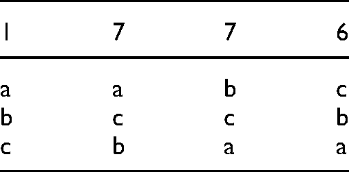
Borda’s (1770) example preference profile showing that plurality suffers from the Condorcet Loser Paradox.
At a presentation at the French Royal Academy of Sciences on June 16th, 1770, the Chevalier de Borda used the example given in Table 1 to point out what is now known as a severe shortcoming of plurality: it may elect a candidate that loses all pairwise majority comparisons. The idea of comparing candidates in terms of pairwise majorities was picked up by Borda’s contemporary the Marquis de Condorcet and has led to a number of influential concepts in social choice theory. A Condorcet winner is a candidate that is preferred to every other candidate by some majority of voters. A voting rule is Condorcet-consistent if it returns the Condorcet winner whenever it exists. Analogously, a Condorcet loser is a candidate that loses all pairwise majority comparisons. Both Condorcet winners and Condorcet losers are unique whenever they exist. In the example given in Table 1, candidate
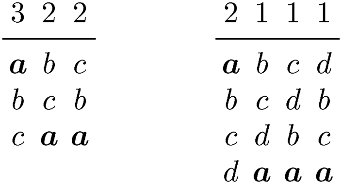
Condorcet Winner Paradox
A candidate is not elected even though it is the Condorcet winner. Condorcet-consistent voting rules are, by definition, immune to this paradox.
Absolute Winner Paradox
A candidate is not elected even though it is ranked first by an absolute majority of voters. This is a special case of the Condorcet Winner Paradox.
Condorcet Loser Paradox
A candidate is elected even though it is a Condorcet loser. Borda’s paradox refers to the Condorcet Loser Paradox for plurality voting.
Absolute Loser Paradox
A candidate is elected even though it is ranked last by an absolute majority of voters. This is a special case of the Condorcet Loser Paradox.
Next, we list multi-profile paradoxes, which require more than one preference profile to materialize.
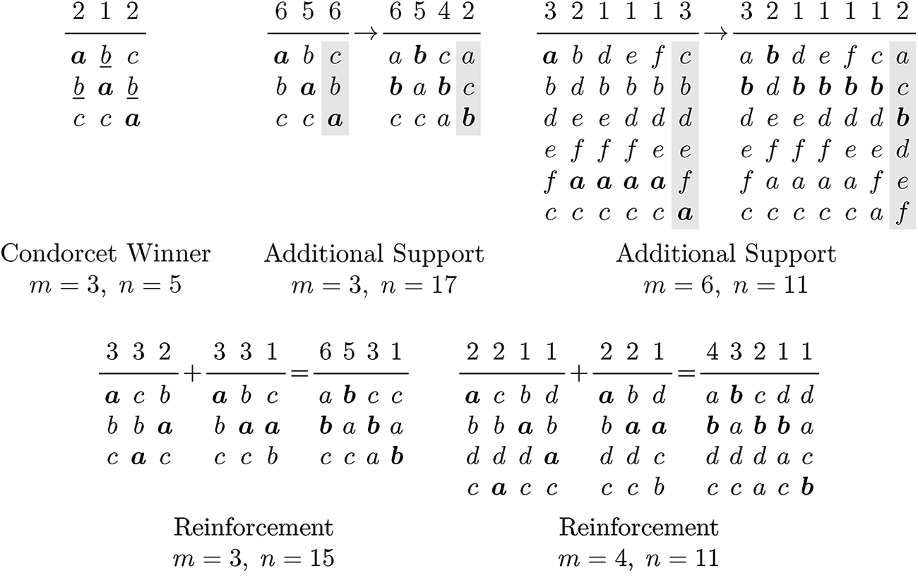
Additional Support Paradox
A candidate wins the election, but loses if it rises in an individual preference ranking while all other individual rankings remain the same. A voting rule that is immune to the Additional Support Paradox is called monotonic. Some voting rules are only susceptible to this paradox if at least two voters change their preferences. In theses case, we will consider a variant of the paradox were two voters with the same preferences consistently change their preferences.
Reinforcement Paradox
A candidate that wins in two preference profiles (e.g., disjoint districts or electorates) is not elected when both preference profiles are merged. A voting rule that is immune to the Reinforcement Paradox is said to satisfy reinforcement.
No-Show Paradox
A voter is better off by abstaining from an election, i.e., he prefers the candidate that is elected in his absence to the one that is elected when he joins the electorate. A stronger version of this paradox, considered by Felsenthal and Nurmi (2019), requires that the candidate that is elected in the voter’s presence is a Condorcet winner. 6 Whenever applicable, we also consider this strengthened variant of the No-Show Paradox and denote it by No-Show + CW. This paradox often also allows for the abstention of a group of like-minded voters with identical preference relations.
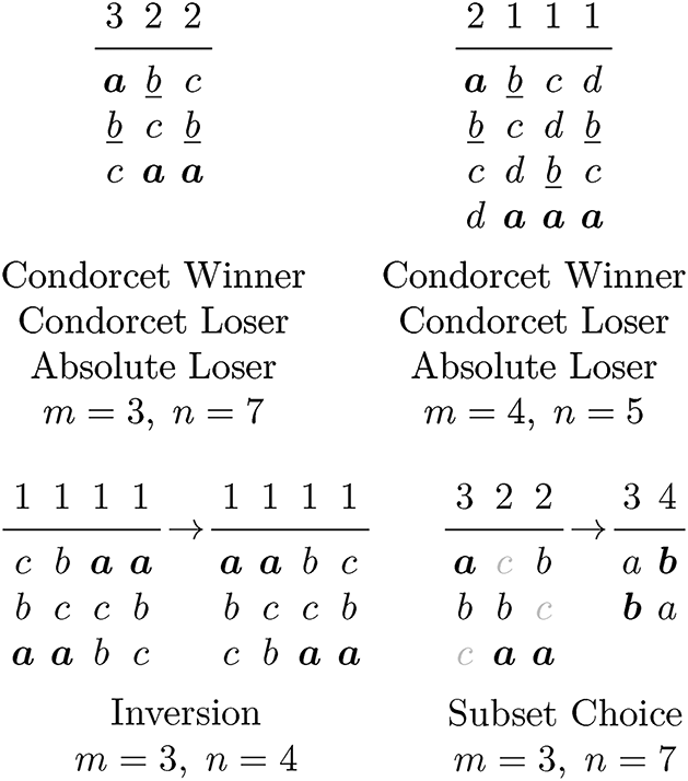
Preference Inversion Paradox
The winner of the election remains the same when all preference rankings are inverted.
Subset Choice Paradox
The winner of the election changes if one of the losing candidates drops out of the election. This paradox is related to classic choice consistency conditions.
In this section, we describe our methodology for finding minimal voting paradoxes. We consider two types of minimality: minimality with respect to the number of voters and minimality with respect to the number of candidates. Our goal is to identify voting paradoxes that are independent of how ties are broken. We therefore only consider preference profiles where the voting rule in question returns a unique winner. 7
Integer linear programming
Integer linear programming (ILP) is an optimization technique that allows the maximization of linear combinations of integer variables subject to constraints given as linear inequalities (see, e.g., Conforti et al., 2014). The maximization objective will only be of secondary interest for our purposes; we rather focus on the feasibility of linear constraints. An integer program is infeasible if it does not admit a solution, i.e., an assignment of the variables, that satisfies the constraints. For the problems we consider, it suffices to only consider binary variables, which is also called 0-1 ILP.
We translate each possible combination of voting rule and paradox for a fixed number of voters and candidates into an ILP such that the program is feasible if and only if there is an instance of the voting paradox. A solution of such an ILP can then be translated to a preference profile exhibiting the paradox. If, on the other hand, the integer linear program is infeasible, this implies that there does not exist a paradox for the given number of voters and candidates. While ILP is an NP-hard problem in general, powerful software packages such as Gurobi Optimization are able to solve considerably large ILPs using sophisticated solving algorithms. This allows us to effectively search for voting paradoxes with up to 10 candidates and 20 voters. 8
ILP formulation of voting paradoxes
We start by introducing the variables representing the preference relations of the voters. Let 

In the following, we will demonstrate how to model a concrete voting paradox using the example of Borda’s paradox, which occurs if there exists a candidate which is first-ranked by a relative majority and happens to be the Condorcet loser. Without loss of generality, we fix candidate
In order to make candidate 


With the help of these variables, we can now add a constraint for each candidate 
We have also experimented with another encoding, in which there is an integer variable for every possible preference relation, representing how many voters share these preferences. Such encodings are also used when determining the frequency of voting paradoxes (see, e.g., Gehrlein, 2006; Gehrlein and Lepelley, 2011, 2017). For our purposes, this encoding performs worse than the one described above because the number of variables grows super-exponentially in the number of candidates. However, as explained in the next section, we utilize this encoding to verify minimality of our instances when the number of candidates is small.
Each of the paradoxes we consider requires at least 3 candidates and at least 2 voters. For each paradox, we seek two kinds of minimal instances. For one, we first minimize the number of candidates
These instances can be found by iteratively generating ILPs and increasing
Minimal instances of Borda’s paradox, where plurality elects the Condorcet loser
While we can guarantee to find the minimal
When first minimizing the number of voters, this is a bit trickier. Many minimal instances only use 3 or 4 voters, which can easily be seen to be the lowest possible number. In the case of Borda’s paradox for example (see Figure 1), it can be verified that no such example with 4 or less voters is possible because, under this condition, a unique plurality winner is top-ranked at least twice and hence cannot be a Condorcet loser. Similar arguments can be made for most other paradoxes. Notable exceptions are the Reinforcement Paradox for the maximin procedure and Young’s rule, the No-Show Paradox for plurality with runoff for the maximin procedure, Kemeny’s rule, and Young’s rule, and the Additional Support Paradox for plurality with runoff. For these paradoxes, we can guarantee that no instance with fewer voters is possible when the number of candidates does not exceed 8.
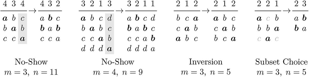
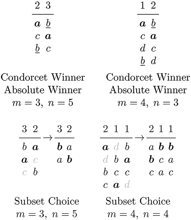
In this section, we present minimal instances of voting paradoxes for 13 common voting rules: plurality, plurality with runoff, instant runoff, Coombs’ method, Bucklin’s method, Borda’s count, Black’s method, Nanson’s method, Baldwin’s method, the maximin procedure, Copeland’s method, Kemeny’s method, and Young’s method. The last seven of these rules are Condorcet-consistent. 9 As already mentioned, we only consider preference profiles in which the voting rule in question returns a unique winner.
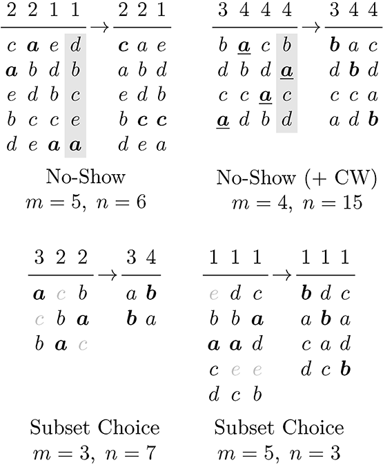
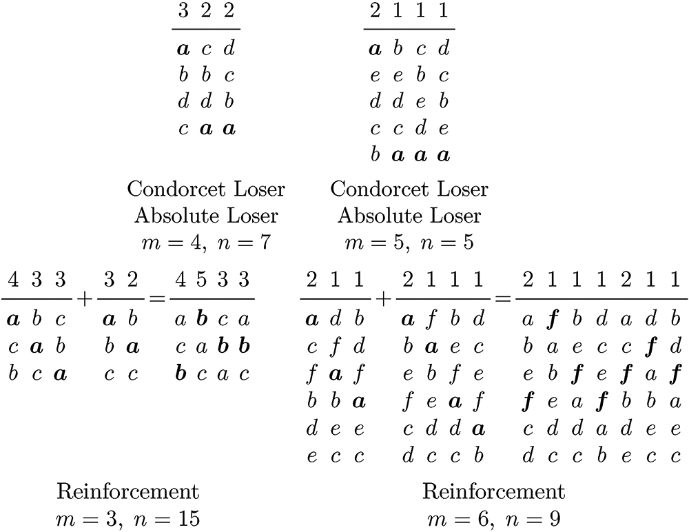
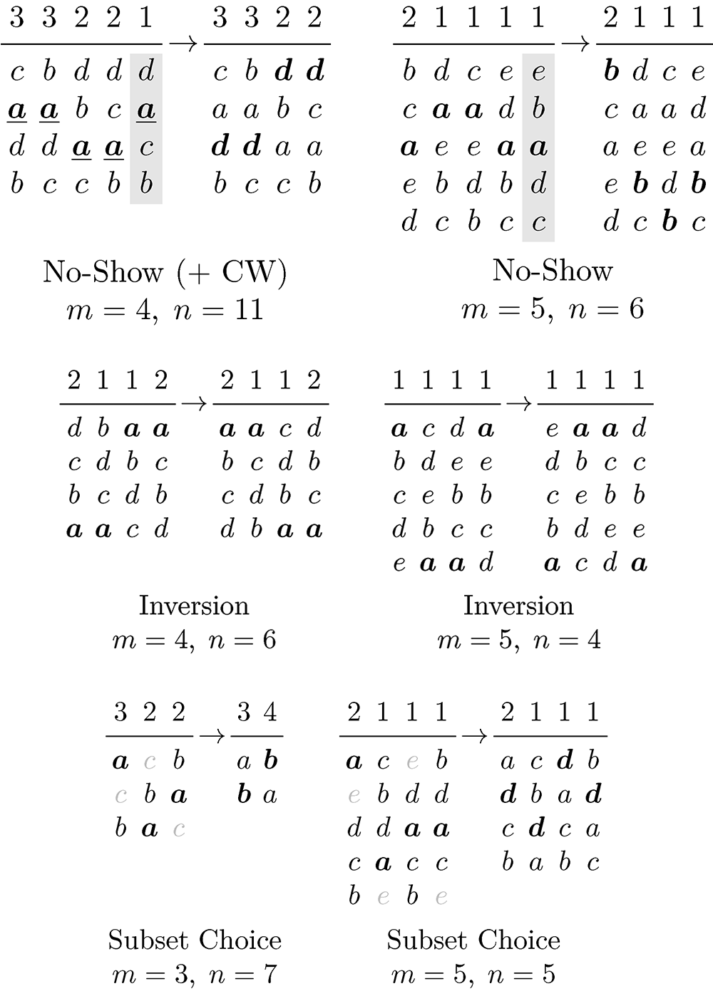
This compilation is complete in the sense that if a voting rule suffers from a given paradox, then we provide an instance that is minimal with respect to the number of voters and an instance that is minimal with respect to the number of candidates. In some cases, these instances coincide. All instances use a minimal number of voter types subject to the other objectives.
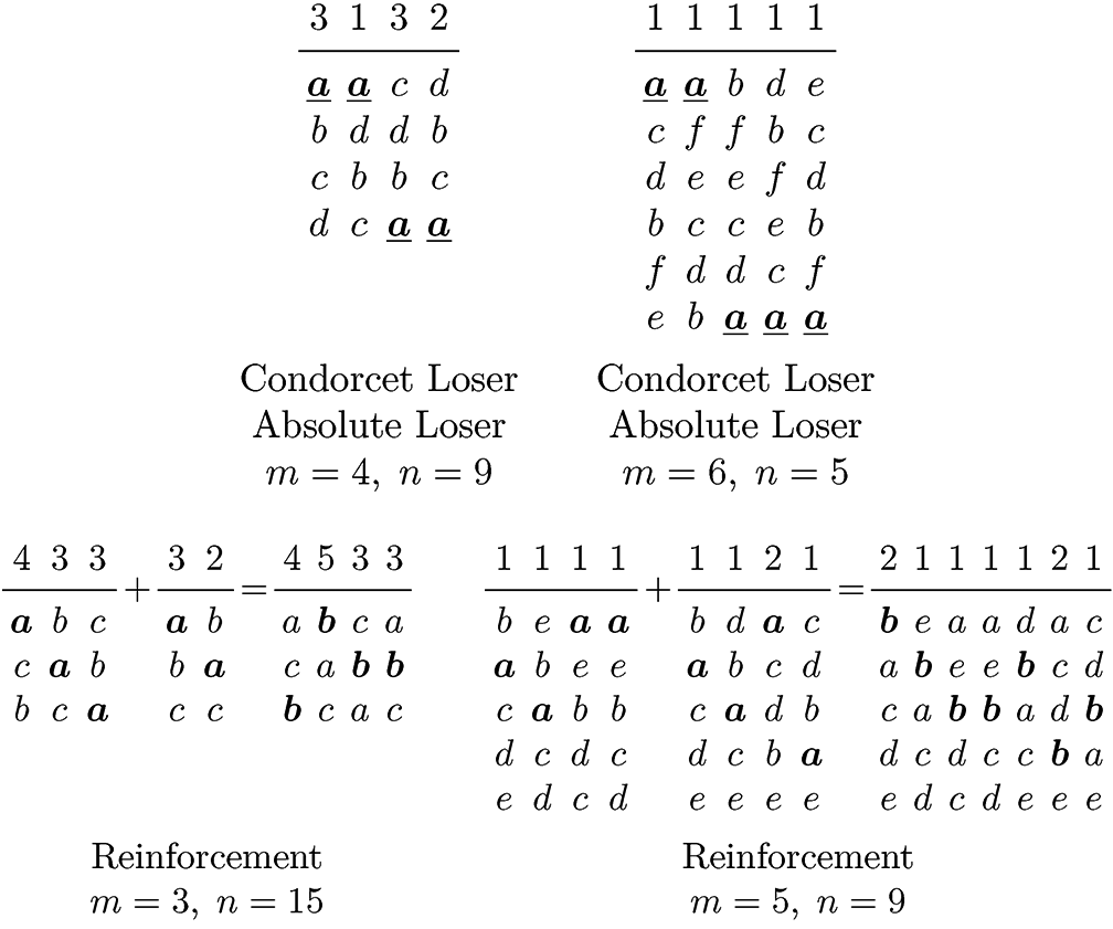
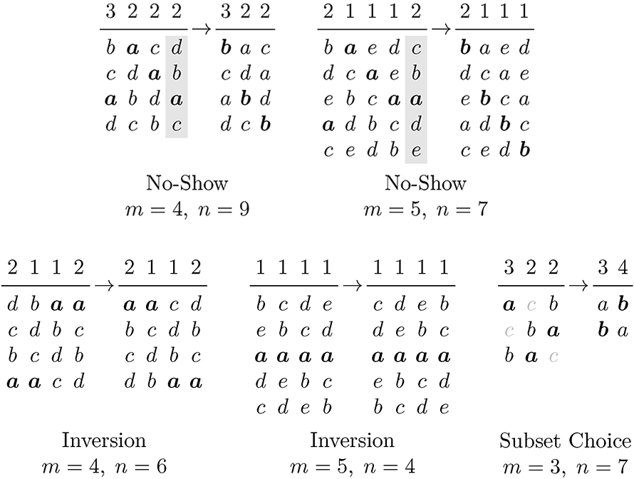
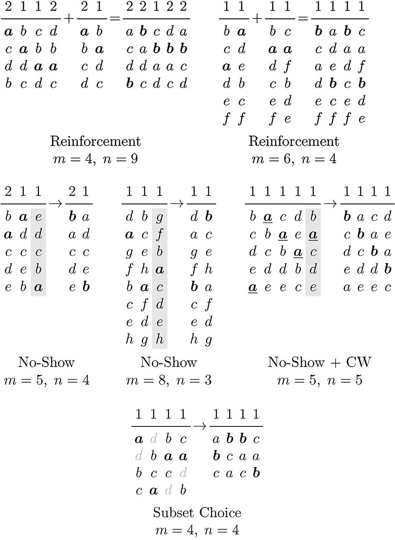
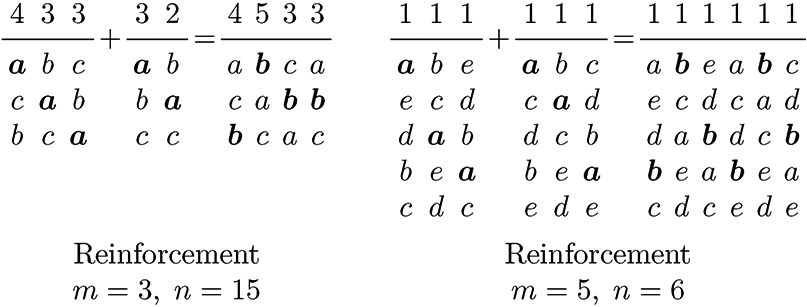
We use the following notation to simplify the depiction of the paradoxes: The winning candidate for a preference profile and voting rule is typeset in bold face. The Condorcet winner or Condorcet loser is underlined whenever this candidate is relevant for the paradox. A candidate that is removed in the Subset Choice Paradox is typeset in gray. For the No-Show Paradox and the Additional Support Paradox, the changed preference relation is highlighted in gray. The correctness of the instances is easily verified (e.g., using the interactive voting platform https://voting.ml).
Plurality
The candidate that is ranked first by most voters (a relative strict majority) is the plurality winner. The minimal voting paradoxes for plurality are relatively straightforward. Note that the first preference profile is an instance for all paradoxes.
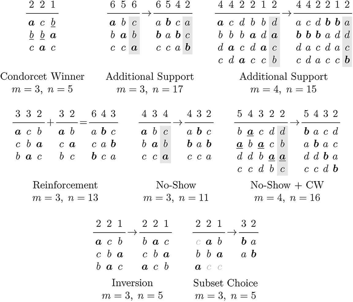
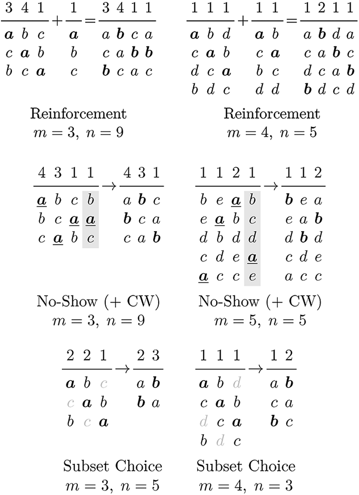
Plurality with runoff
All candidates except the two that are ranked first by most voters are eliminated from the ballot. The candidate preferred by a majority in the resulting ballot is elected. (It follows that a candidate that is ranked first by an absolute majority of voters on the original ballot will be elected immediately.) In order to obtain instances that are independent of any tie-breaking mechanism, we only consider preference profiles where there are exactly two candidates which are ranked more often than any other candidate. Avoiding ties implies that the Additional Support Paradox may only appear if at least two voters change their preferences.
Plurality with runoff is only prone to the No-Show Paradox if at least two voters abstain, given our restriction that there must be a unique winner. For this reason, we here consider the No-Show Paradox when two voters with identical preferences abstain.
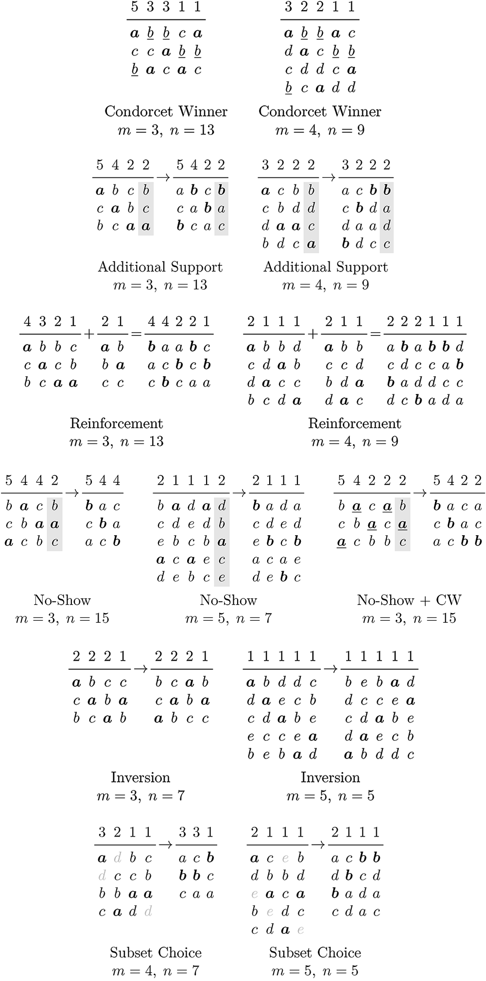
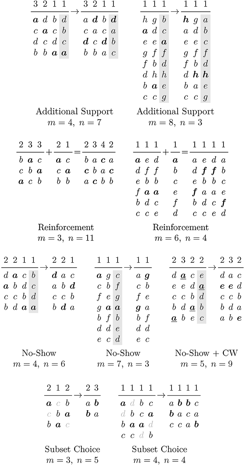
Instant runoff
A candidate ranked first by an absolute majority of voters is elected immediately. Otherwise, the candidate ranked first by the smallest number of voters is eliminated from the ballot. This step is repeated until there is a candidate which is ranked first by an absolute majority of voters. Instant runoff is also known as the alternative vote procedure or ranked-choice voting.
If there are several candidates ranked first by a minimal number of voters, the candidate to be eliminated can be determined using a tie-breaking rule. In order to obtain instances that are independent of any such tie-breaking, we only consider preference profiles in which no ties of this kind occur at any iteration. Note that as a consequence, the No-Show paradox and the Additional Support paradox may only appear if at least two voters abstain or change their preferences, respectively. Remarkably, the No-Show Paradox can also occur if the winner in the initial profile is a Condorcet Winner, which shows that Felsenthal and Nurmi’s (2019) claim to the contrary is incorrect. 10
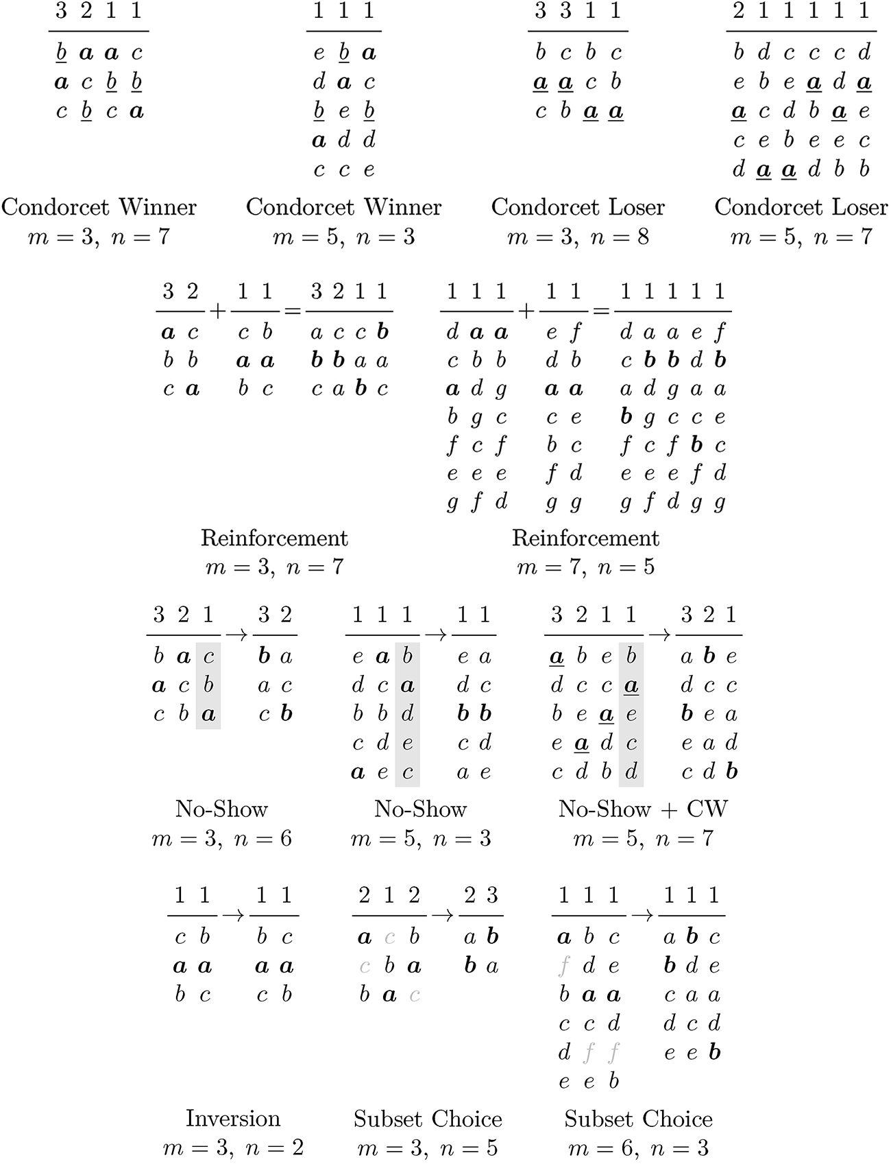
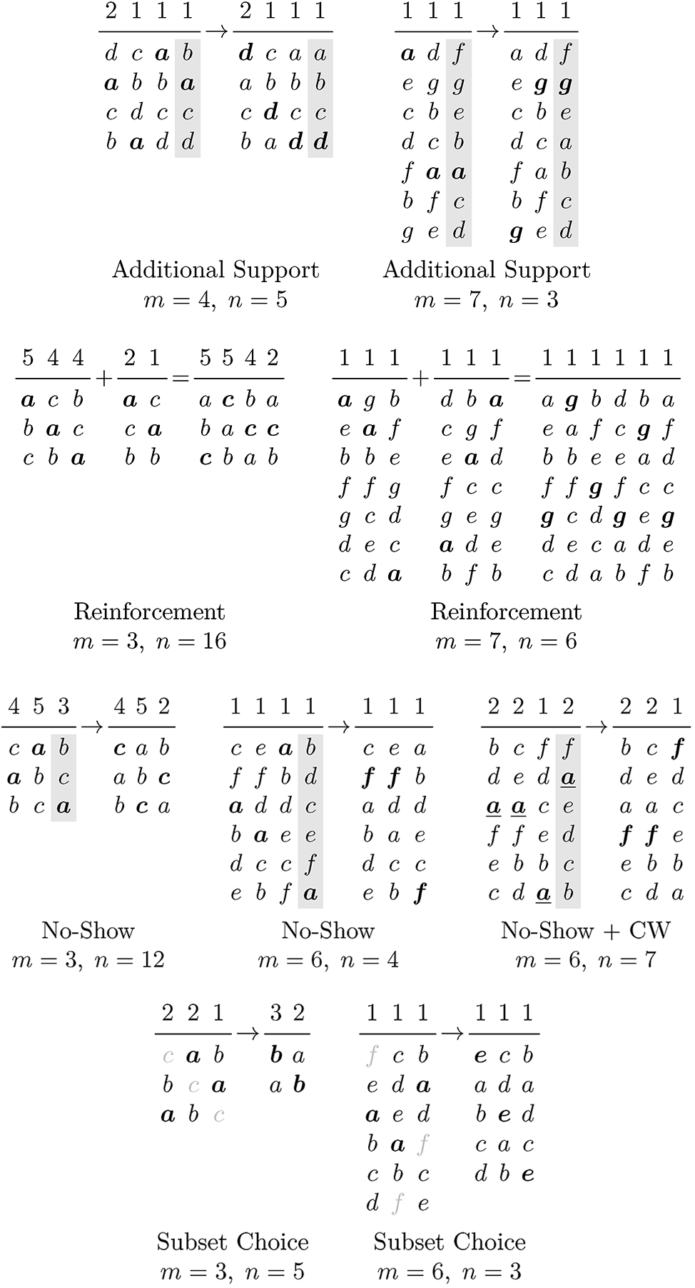
Coombs’ method
A candidate ranked first by an absolute majority of voters is elected immediately. Otherwise, the candidate ranked last by the largest number of voters is eliminated from the ballot. This step is repeated until there is a candidate which is ranked first by an absolute majority of voters. If there are several candidates ranked last by a maximal number of voters, the candidate to be eliminated can be determined using a tie-breaking rule. In order to obtain instances that are independent of any such tie-breaking, we only consider preference profiles in which no ties of this kind occur at any iteration. Note that as a consequence, the No-Show Paradox and the Additional Support Paradox may only appear if at least two voters abstain or change their preferences, respectively.
Bucklin’s method
A candidate ranked first by an absolute majority of voters is elected immediately. Otherwise, a candidate that is ranked first or second by the largest absolute majority of voters is elected. If no such candidate exists, one considers the first three ranks, and so on.
Remarkably, the No-Show Paradox can also occur if the winner in the initial profile is a Condorcet Winner, which shows that Felsenthal and Nurmi’s (2019) claim to the contrary is incorrect. 11
Borda’s count
Given a preference relation, let the rank of a candidate be the number of candidates that are ranked below that candidate. The Borda score of a candidate is the sum of all of its ranks in the preference profile. The candidate with the highest Borda score wins the Borda count.
Black’s method
If there is a Condorcet winner, it is elected. Otherwise, Borda’s count is used to determine the winning candidate.
Nanson’s method
Nanson’s method is a multi-round elimination method, where in each round, all candidates whose Borda score is not strictly larger than the average Borda score (
Baldwin’s method
Baldwin’s method is a multi-round elimination method similar to Nanson’s method, where in each round all candidates with the the lowest Borda score are eliminated until a single candidate remains. This candidate is the winner.
Baldwin’s method is sometimes also called the Borda Elimination Rule.
Maximin procedure
The majority margin for two candidates
The maximin procedure is only prone to the No-Show Paradox if at least two voters abstain, given our restriction that there must be a unique winner. For this reason, we here consider the No-Show Paradox when two voters with identical preferences abstain. When also considering preference profiles that do not admit a unique maximin winner, Brandt et al. (2017) have shown that, no matter how ties are broken, the maximin procedure suffers from the No-Show Paradox whenever there are at least 7 voters and 4 candidates.
Copeland’s method
For each pair of candidates, assign a point to the candidate that is preferred to the other candidate by more than half of the voters and half a point to both if there is a majority tie. The candidate with the highest score wins.
Kemeny’s method
Kemeny’s rule is based on computing a consensus ranking, i.e., a ranking in which as many pairwise comparisons as possible coincide with the preferences of the voters. The top-ranked alternative of the consensus ranking is the winner.
When also considering preference profiles that do not admit a unique Kemeny winner, Brandt et al. (2017) have shown that, no matter how ties are broken, Kemeny’s method suffers from the No-Show Paradox whenever there are at least 4 voters and 4 candidates.
Kemeny’s rule even suffers from the No-Show Paradox in the presence of a Condorcet winner when allowing the abstention of several voters with identical preferences.
Young’s method
For each candidate, determine the minimal number of voters which need to be removed such that this candidate becomes the Condorcet winner. The candidate with the smallest such score is the winner. 12
Conclusion and discussion
We have conducted an exhaustive analysis of minimal voting paradoxes for 13 common voting rules. Our results are summarized in Table 2. Almost all of the minimal instances we found are smaller than instances that have appeared in the literature. Of course, if an instance uses fewer voters and/or candidates it does not necessarily have to be more effective or more revealing. However, most of our examples also use fewer types of voters, which hopefully helps to grasp the structural causes of these paradoxes. The results in Table 2 can also be leveraged to argue for certain rules when the numbers of voters or candidates are severely restricted.
Sizes of minimal voting paradoxes. There are two instances for each paradox and voting rule (displayed in separate rows). The first instance minimizes the number of candidates and then the number of voters; the second one minimizes the number of voters and then the number of candidates. For each instance, we first give the number of candidates
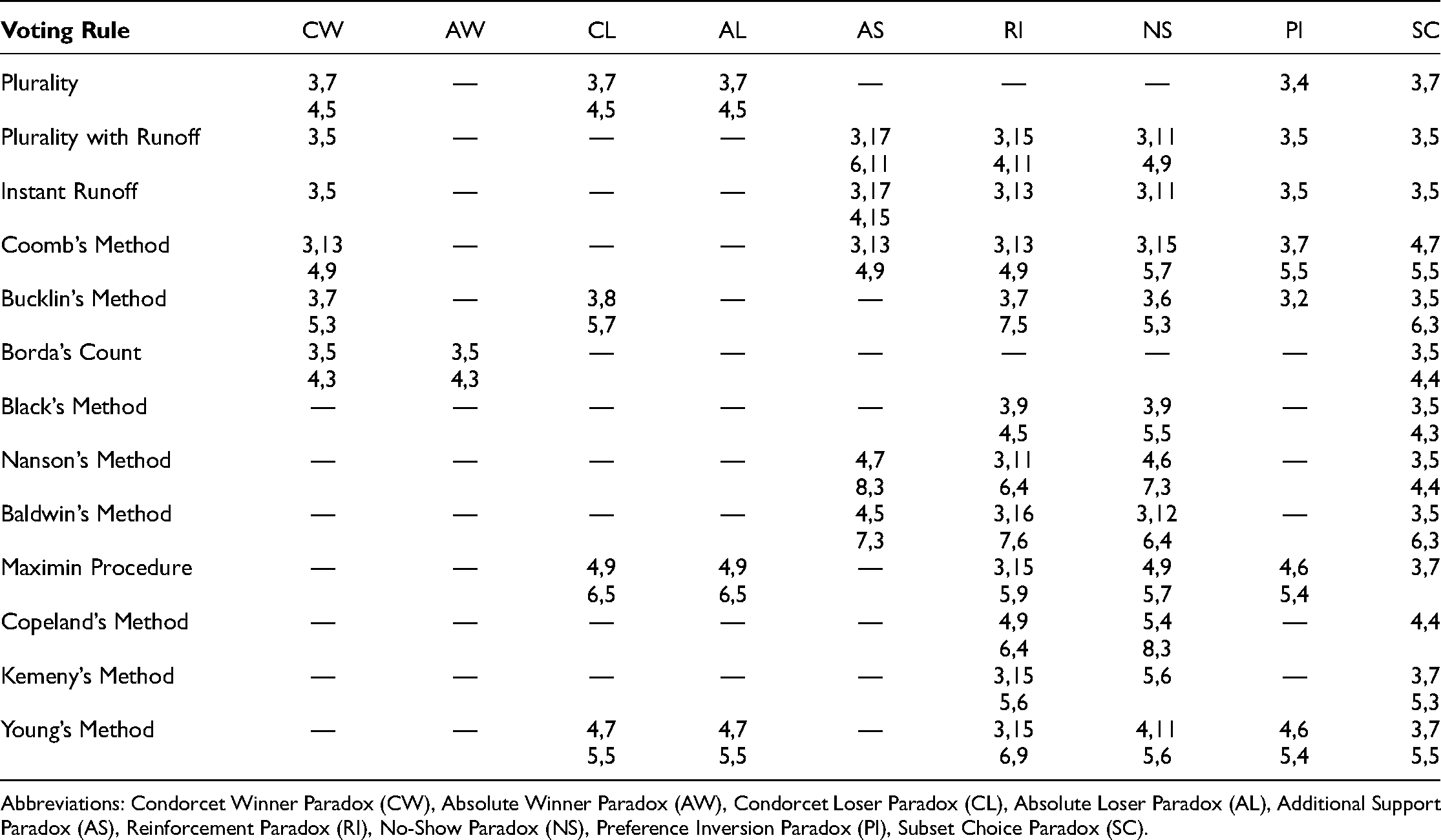
Abbreviations: Condorcet Winner Paradox (CW), Absolute Winner Paradox (AW), Condorcet Loser Paradox (CL), Absolute Loser Paradox (AL), Additional Support Paradox (AS), Reinforcement Paradox (RI), No-Show Paradox (NS), Preference Inversion Paradox (PI), Subset Choice Paradox (SC).
For example, consider the important special case of 3 candidates and arbitrarily many voters. In this case, two voting rules stand out. The first one is Copeland’s method, which does not suffer from any of the considered voting paradoxes. However, it should be noted that, to some extent, this is an artefact of restricting attention to preference profiles that admit a unique winner and Copeland’s indecisiveness. Any single-valued rule that always returns a candidate from the set of Copeland winners will exhibit the Reinforcement Paradox and the Subset Choice Paradox. For the No-Show Paradox, this depends on how ties between Copeland winners are broken. This brings us to the maximin Procedure, which is immune to the No-Show Paradox when there are only 3 candidates (Moulin, 1988). Moreover, the Reinforcement Paradox—while possible in principle—only occurs with very low probability (Courtin et al., 2014; Plassmann and Tideman, 2014; Heilmaier, 2020). It is not difficult to show that for 3 candidates, the maximin procedure is equivalent to Kemeny’s method and Young’s method (as well as a number of other rules such as Schulze’s rule, ranked pairs, split cycle, and Dodgson’s procedure, which we do not consider here). Unless there are ties, this also holds for Nanson’s method, which is slightly more selective. Nanson’s method, which was proposed as early as 1883, allows for a relatively simple description in the case of 3 alternatives: each voter assigns 2 points to his most-preferred candidate and 1 point to his second most-preferred candidate; all candidates whose score exceeds the total number of voters face off in a runoff election (Nanson, 1883). We believe that this rule is quite attractive for 3-candidate elections (see, also, Nurmi, 1989; Felsenthal and Nurmi, 2018; Lepelley and Smaoui, 2019: who draw similar conclusions). 13
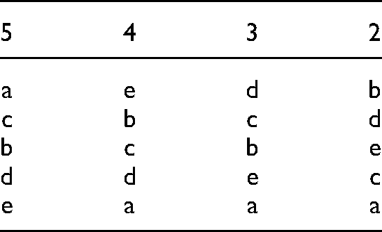
A big advantage of our systematic approach for generating voting paradoxes is its flexibility. It is easily possible to adapt our implementation to identify other paradoxes or voting phenomena. For example, an astonishing example by Balinski (2002) shows that five voting rules—all of which are used for real-world elections—yield five different winners for the very same preferences. 14 Balinski’s example uses 100 voters and 6 different types of voters. We have shown that the minimal preference profile of this kind requires 14 voters and 4 types of voters (see Table 3). 15 Examples like this can be used to great effect when introducing laypersons as well as scholars to the difficulty of making social choices.
Five voting rules, five winners. Plurality elects candidate
Finally, to end on a positive note, we would like to conclude by mentioning that all of the considered paradoxes can be avoided by allowing for randomization when picking the election winner. A randomized rule, proposed by Fishburn (1984), circumvents appropriate extensions of the paradoxes to the randomized voting setting. This rule is called maximal lotteries and can be characterized using axioms that basically prohibit vulnerability to phenomena such as the Reinforcement Paradox or the No-Show Paradox (Brandl et al., 2016, 2019; Brandl and Brandt, 2020). Maximal lotteries always assign probability 1 to Condorcet winners and probability 0 to Condorcet losers (avoiding the Condorcet Winner, Absolute Winner, Condorcet Loser, and Absolute Loser Paradoxes). A candidate that is elected with positive probability will still be elected with positive probability when he is reinforced (avoiding the Additional Support Paradox). 16 No group of voters can obtain more utility by abstaining from an election for all utility functions consistent with their ordinal preferences (avoiding the No-Show Paradox). 17 A candidate that will be elected with probability 1 will be elected with probability 0 when all preference rankings are inverted (avoiding the Preference Inversion Paradox). 18 In almost all preference profiles (namely whenever there is a unique maximal lottery), the following two statements hold as well. If the same lottery is returned for two preference profiles, this lottery will also be returned when both preference profiles are merged (avoiding the Reinforcement Paradox). Finally, a maximal lottery is unaffected by removing losing candidates (avoiding the Subset Choice Paradox).
Footnotes
Acknowledgements
The authors are indebted to Hannu Nurmi and Christian Stricker for helpful feedback and discussions.
Declaration of Conflicting Interests
The author(s) declared no potential conflicts of interest with respect to the research, authorship, and/or publication of this article.
Funding
The author(s) disclosed receipt of the following financial support for the research, authorship, and/or publication of this article: This material is based on work supported by the Deutsche Forschungsgemeinschaft under grant BR 2312/12-1.