Sage Journals: Discover world-class research

Abstract

The response patterns across the fieldwork period are analyzed in the context of a panel study with a sequential mixed-mode design including a self-administered online questionnaire and a computer-assisted telephone interview. Since the timing of participation is modelled as a stochastic process of individuals’ response behaviour, event history analysis is applied to reveal time-constant and time-varying factors that influence this process. Different distributions of panelists’ propensity for taking part in the web-based survey or, alternatively, in the computer-assisted telephone interview can be considered by hazard rate analysis. Piecewise constant rate models and analysis of sub-episodes demonstrate that it is possible to describe the time-related development of response rates by reference to individuals’ characteristics, resources and abilities, as well as panelists’ experience with previous panel waves. Finally, it is shown that exogenous factors, such as a mixed-mode survey design, the incentives offered to participants and the reminders that are sent out, contribute significantly to time-related response after the invitation to participate in a survey with a sequential mixed-mode design. Overall, this contribution calls for a dynamic analysis of response behaviour instead of the categorization of response groups.

Keywords

Computer-assisted survey research computer-assisted telephone interview computer-assisted web-based interview event history analysis panel data survey response time timing of participation

Introduction

Current research on computer-assisted survey methods investigates both the response rate as well as the timing of participation in web surveys and other survey modes (Callegaro et al., 2014; Dillman et al., 2009; Göritz & Stieger, 2009; Gummer & Struminskaya, 2020; Rao & Pennington, 2013; Tourangeau et al., 2013; Van Mol, 2017). This focus continues a long tradition of research on this issue (Becker et al., 2019; Chebat & Cohen, 1993; Göritz, 2014; Houston & Ford, 1976; Huxley, 1980; Rao & Pennington, 2013). However, there are only a few empirical studies that are concerned with the time dimension of the participation in computer-assisted surveys. It is interesting to know how long it takes for invitees to respond to a researcher’s request that they take part in a survey (Faria & Dickinson, 1992, p. 51; Rao & Pennington, 2013, p. 652). How can one shorten the time that elapses before invitees respond? The distribution of the speed of response – that is, the time that elapses between the researchers’ invitation and the invitees’ response in an online survey or computer-assisted telephone interview – among the target sample provides important information for the survey management in regard to cost calculations, sending follow-ups, offering additional incentives, switching to another survey mode, and the final response rate (Becker et al., 2019; Gummer & Struminskaya, 2020; In Lynn, 2009; Truell et al., 2002).

In regard to the distribution of the speed of response to a request, on the one hand there are several studies which distinguish between ‘early’ and ‘late’ respondents; on the other hand, there are few studies which analyze the time-related processes and events in the fieldwork period in a theoretically and methodologically adequate way (Becker et al., 2019; Becker & Glauser, 2018; Chebat & Cohen, 1993; Sauermann & Roach, 2013; Van Selm & Jankowski, 2006). Those studies that do exist demonstrate, indirectly at least, that epistemological uncertainty is encountered when one seeks to distinguish between ‘early’ and ‘late’ respondents (Green, 2014; Kreuter et al., 2014; Lugtig, 2014; Rao & Pennington, 2013; Sigman et al., 2014). First, the definition of these types of respondents is inconclusive, across these studies (Klingwort et al., 2018, p. 4). Second, in several studies, there are different operationalizations of these respondent groups.1 However, these harbour some problems. Due to different value ranges, the definitions are incompatible, due to different fieldwork period durations. Thus, because of different standards of time, it is not possible to compare the findings across surveys. This is also the case for the classification of response groups by reminders: the results for response groups depend on the point in time at which reminders are sent out, which vary across surveys (Sigman et al., 2014, p. 654). Third, the categorization and operationalizations used in these studies are theoretically arbitrary since they are not based on arguments that are deduced from a well-established theory of survey participation (Singer, 2011). They do not contribute to explanations of the timing of survey participation, response speed across target groups and consequences within the fieldwork period. Fourth, there are methodological issues in these studies using such classifications of response groups. These issues arise because these studies are based on a comparative-static view and the use of statistical procedures that are suited for cross-sectional data. Thus, existing findings are often misleading (Chebat & Cohen, 1993; Sauermann & Roach, 2013; Sigman et al., 2014). For example, it cannot be ruled out that target persons would have answered the survey invitation if the fieldwork phase had been longer. Overall, this problem of right-censored cases is not taken into account by cross-sectional designs. The existing findings are also invalid because both the timing of survey participation and the response rate varies within a survey at different time-related stages of the fieldwork (Becker & Glauser, 2018), as well as between surveys or waves within a panel study (Becker et al., 2019). It is observed that the value ranges for ‘early’ and ‘late’ respondents across several studies overlap. Consequently, the definition of respondent groups varies systematically between either surveys or survey modes, and therefore becomes meaningless. Fifth, and finally, studies offer a poor record in terms of the comparison of ‘late’ respondents with non-respondents, in order to detect the ‘causes’ of, or ‘reasons’ for, non-response bias (Chen et al., 2003, p. 200; Lahaut et al., 2002, p. 133; Studer et al., 2013, p. 316). In general, this comparison is based on an inadequate design and on the wrong reference groups. It is made using a cross-sectional design after the entirety of the fieldwork. However, it has to be considered that responses can occur at any point in time. Therefore, we need comparisons between (potential) respondents and non-respondents at any point in time at which responses take place, regardless of whether respondents are ‘early’ or ‘late’, in order to understand the occurrence of non-response bias.

In other words, there is a question as to whether we need such a classification of response groups. What we need is a theoretically driven and methodically sound analysis of response behaviour across the fieldwork period. From a dynamic longitudinal perspective, there is a need to analyze both dimensions: the timing of survey participation as a stochastic process of individuals’ decisions, and the response rate, as its time-dependent consequence (Singer, 2006, p. 640; Tourangeau et al., 2013, p. 38). There are several reasons for this requirement. From the theoretical angle, analysis of the timing and extent of survey participation contribute to an (indirect) empirical test of theoretical approaches that strives to answer the question of when and why individuals take part in scientific surveys. From the methodological angle, the process of survey participation can be described more realistically by taking into account time-constant factors (e.g. gender) and time-varying covariates (e.g. consecutive reminders, the weather situation) on different analytical levels – micro, meso and macro levels (Blossfeld, 1996). By considering time-varying covariates in an event-oriented design, it is possible to reveal the causalities of this stochastic process of survey response (Blossfeld & Rohwer, 1997). From a statistical angle, event history analysis provides techniques and procedures for handling these theoretical and methodological premises (Blossfeld et al., 2019). There currently exist a few studies that demonstrate the validity of this claim (Becker et al., 2019; Becker & Glauser, 2018; Chebat & Cohen, 1993; Durrant, D’Arrigo, & Steele, 2013, Durrant, D’Arrigo, & Müller, 2013; Sauermann & Roach, 2013). From a practical angle, evidence-based in-depth knowledge of participation timing, consisting of the time interval between survey launch and first response, as well as of the rate of survey participation at any point in time until the end of fieldwork, is useful for rational survey management and efficient organization (Gummer & Struminskaya, 2020, p. 19). For example, it contributes to improving the efficiency of fieldwork as well as savings in terms of survey time and costs (Lipps et al., 2019).

In order to demonstrate the benefits of a dynamic investigation of the timing of survey participation based on event history analysis, the following questions have to be answered: How long does it take for a number of individuals to reciprocate the invitation to participate in a survey? Which factors – such as invitees’ resources and abilities, or features of the survey management (e.g. follow-up invitations and reminders) – contribute to the timing of individuals’ survey participation? What can researchers do to reduce respondents’ delay in responding to a survey, and the related duration of the fieldwork period? In regard to the inducement of a quicker response rate and the effect of several strategies (such as invitation, reminders and incentives) on individuals’ enhanced survey response, these three questions address one of the main research problems in the area of survey methodology.

Theoretical Consideration

Since participation in a survey is voluntary, the individuals who are asked to take part are free to accept or reject that request (Groves & Couper, 1998, p. 1). Their decision regarding survey participation is thus based on their ‘free will’ (Blossfeld, 1996, p. 197). Therefore, they can choose their own time to respond to the request (Groves & Couper, 1998, p. 32). They can respond immediately after the invitation, at a later more convenient point in time or never. Thus, survey participation, as observed by social researchers, is the result of individuals’ decisions and can occur at any point in time (Sigman et al., 2014). Survey participation therefore has to be modelled as a time-continuous, discrete-state stochastic process (Singer, 2006). Such a probability process presupposes the mathematical description of timely ordered and random proceedings. Stochastic phenomena are events that develop over time (Aalen et al., 2008, p. 23). A response, as an event, can occur at any point in time across the fieldwork period and is not restricted to a predetermined point in time. Furthermore, there are time-constant factors (e.g. gender and social origin) and/or time-dependent factors (e.g. follow-ups and time restrictions) that influence the outcome and timing of events, such as survey participation, at any time (Blossfeld & Rohwer, 1997, p. 361). In this respect, the response rate of a survey is the consequence of the history of invitees’ responses, which consists of events such as a response occurring over discrete or continuous time in the fieldwork period for a number of individuals who are eligible for survey participation. The invitees’ response speed – that is, the timing of their survey participation – is a function of the time that elapses between the researchers’ invitation until the target persons’ response. Thus, an analysis of response speed has to take the timing and the number of responses into account simultaneously (Chebat & Cohen, 1993, p. 21).

The techniques and statistical procedures of event history analysis can be used for dynamic analysis related to the timing of events such as survey response (Aalen et al., 2008). Event history analysis involves statistical methods for analyzing stochastic processes with discrete states, such as survey response, and continuous time, such as time elapsed in the fieldwork after survey launch (Blossfeld et al., 2019; Kalbfleisch & Prentice, 2002). Thus, event history models might be particularly helpful instruments because they allow a time-related empirical representation of the theoretical arguments in regard to the structure, number and timing of survey participation (Blossfeld & Rohwer, 1997, p. 363). From a theoretical viewpoint, only time-changing variables provide the most convincing empirical evidence of the invitees’ propensity to take part, in terms of the transition to response.

Understanding and explaining social processes, such as the propensity for survey response, by time-related specification of the past and present conditions under which individuals with a ‘free will’ obviously act, the preferences individuals pursue at the present time and beliefs and expectations guiding their survey behaviour, and the survey response that probably will follow immediately or in the future have to take into account. This means that such an event occurs contingent on previous events and the stochastic process initiated by previous events, such as invitations, incentives or reminders. In sum, the aim of this kind of modelling as applied in the present contribution is to specify the likelihood of survey participation – that is, the hazard rate – as a stochastic and time-variant function of individual resources and the settings of the survey. This hazard rate $r (t)$ is defined as the marginal value of the conditional probability of such an event occurring – namely, the invitees’ response to an invitation to take part in a survey – in the time interval $(t, t + Δ t)$ , given that this event has not occurred before time $t$ (Blossfeld et al., 2019: 29). Using this statistical procedure, it is possible to reveal the causal impacts of $x$ for the probable occurrence of an event $y$ , such as survey participation: $∆ X_{t} \to ∆ \Pr (∆ Y_{t^{'}}) \to ∆ r (t^{'}), t < t^{'}$ , whereby $t < t^{'}$ .

Given that $T_{y}$ is a random variable indicating the point in time when the event y (survey participation) occurs, it is true that a change in variable Y at time t defines $T_{y} = t$ . The transition rate is formalized as follows (Blossfeld et al., 2019, p. 28):

\Pr (t \leq T_{y} < t^{'} | T_{y} \geq t)

This probability reflects the fact that an event y occurs in the time interval from $t$ to $t ’$ provided that this event has not occurred before in the time interval from $0$ to $t$ . In order to take the future process into account additionally to the process observed in the past, the ratio of the transition probability to the tenure of the time interval indicates the probability of future changes in the dependent variable per unit of time (Blossfeld et al., 2019, p. 28): $\Pr (t \leq T_{y} < t^{'} | T_{y} \geq t) / (t^{'} - t)$ . Since $t ’$ approaches $t$ , the transition rate (or hazard rate) is defined by the following equation:

r (t) = \lim_{t^{'} \to t} \frac{\Pr (t \leq T_{y} < t^{'} | T_{y} \geq t)}{t^{'} - t} .

According to Blossfeld et al. (2019: 29), this transition rate can be interpreted as the actors’ propensity to change state, such as from non-response to response. This propensity is defined in relation to a risk set at moment $t$ – that is, the set of individuals who do not respond until $t$ and, therefore, can respond since they did not respond before $t$ . At each point in time, the transition rate connects the previous events, such as response in the closed past, with the open future. Since the intensity of possible future changes at each point in time is analyzed by the transition rate, it is obvious that this tool is well-suited for describing stochastic processes in terms of the distribution of (potential) survey participation since the survey launch. In other words, event history analysis provides statistic procedures which are appropriate for the estimation of competing risks such as survey response or choice of survey modes.

Parametrical estimations of hazard rates are particularly appropriate for this aim. For fine-grained parametric analysis of the speed and time-dependent selectivity of response, the piecewise constant exponential model will be utilized. According to Blossfeld et al. (2019, p. 124), the ‘basic idea is to split the time axis into time periods and to assume that transition rates are constant in each of these intervals but can change between them’. Using this model makes it possible to analyze the participation pattern in the initial phase of fieldwork in comparison to the other phases of the entirety of the fieldwork period. Applying this procedure, the socially selective differences between ‘early’ and ‘late’ participants are analyzed across time within the fieldwork period. Given theoretically defined time periods, the transition rate for survey participation is defined as follows:

r_{k} (t) = \exp {\bar{α} \begin{array}{c} (k) \\ I \end{array} + A^{(k)} α^{(k)}} i f t \in I_{t},

whereby k is the destination, I is the time interval,

\bar{α} \begin{array}{c} (k) \\ I \end{array}

is a constant coefficient associated with the l^th time period,

A^{(k)}

is a vector of covariates and

α^{(k)}

is an associated vector of coefficients assumed not to vary across time (Blossfeld et al., 2019, p. 125). In particular, it is possible to reveal whether the sample responding in the initial stages of the fieldwork period is different from the sample responding in later stages.

Additionally, using non-parametrical procedures such as the Kaplan–Meier method of calculating the product-limit estimator, the pattern of response across waiting time and its speed since the invitation to the current wave are described on the basis of relative prevalence across time. By calculating indices, such as the median or other quantiles (quartiles or percentiles), it is possible to show how long it takes a number of panelists to respond. The median value, for example, shows how long it takes till 50 per cent of the eligible invitees have responded. In this way, ‘early’ and ‘late’ panelists can be distinguished empirically for descriptive purposes, on a continuous scale, instead of based on arbitrary cutoffs. Furthermore, it is then possible to compare the points in time at which survey participation occurs and the development of the response rate across the timeline of the fieldwork period and between different surveys.

According to Schuster et al. (2020), estimations can be biased systematically when competing events such as the choice of survey modes offered to invitees – that is two or more cause-specific hazards (Kalbfleisch & Prentice, 2002) – are ignored in the analysis of survival data. Against the background of competing risk – the potentially simultaneous occurrence of mutually exclusive events, such as participation in the online mode versus the computer-assisted telephone interview (CATI) mode – the traditional survival analysis (i.e. Kaplan–Meier product-limit estimations) is inadequate to describe the timing and rate of survey participation. The assumption of standard survival analysis, namely, that the censoring of events (i.e. their non-occurrence) is independent, is not valid in this case. Thus, the Kaplan–Meier estimator is biased since the probability of the event of primary interest is overestimated (Noordzij et al., 2013, p. 2672). The overestimation of probabilities increases with the running risk time. Therefore, alternative non-parametric procedures of competing risk analysis – the cumulative incidence competing risk method – are used to describe the patterns of panelists’ participation across the fieldwork period. Since Kaplan–Meier plots are biased in the presence of competing risks, the cause-specific cumulative incidence function (CIF), which is the probability of using a specific survey mode offered before the end of fieldwork period $t$ , should be estimated in order to reveal the risk of choosing one of the competing survey modes (Lambert, 2017). The CIF describes the incidence of the occurrence of an event while taking competing risks into account (Austin & Fine, 2017, p. 4293).

For the multivariate analysis of the competing risks in terms of participation in the online survey versus CATI, the exponential model – $r (t | x (t)) = \exp (β ’ x (t))$ – is equivalent to the proportional cause-specific hazards model suggested by Kalbfleisch and Prentice (2002).2 According to Schuster et al. (2020, p. 44), the ‘cause-specific hazard denotes the instantaneous rate of occurrence of the event of interest in a setting in which subjects can also experience the competing event’. Since this hazard is estimated by removing individuals from the risk set the moment they experience the competing event, meaning that competing events are treated as censored observations, it is possible to estimate the cause-specific hazard using an exponential model in which all events other than the event of interest are treated as censoring. Schuster et al. (2020, p. 44) suggest interpreting these hazard ratios ‘among subjects who did not (yet) experience the event of interest or a competing event. As the cause-specific hazard is directly quantified among subjects that are actually at risk of developing the event of interest, the cause-specific hazard model is considered more appropriate for etiological research’. This is realized by calculating estimations of survey participation separately for the different modes. According to Lunn and McNeil (1995, p. 524), these methods provide the drawback ‘that [they do] not treat the different types of failures jointly, complicating the comparison of parameter estimates corresponding to different failure types’.

Another approach – the sub-distribution hazards approach proposed by Fine and Gray (1999) – is often seen as the most appropriate method to use for analyzing competing risks. In contrast to the cause-specific hazards model, ‘subjects who experience a competing event remain in the risk set (instead of being censored), although they are in fact no longer at risk of the event of interest’ (Noordzij et al., 2013, p. 2673). This precondition is necessary in order to establish the direct link between the covariates and the CIF to predict the hazard ratios. However, this makes it difficult to interpret them in a straightforward way and is therefore not appropriate for etiological research (Schuster et al., 2020, p. 44). By taking competing risks into account, the coefficients estimated by the stcrreg module implemented in the statistical package Stata can be used to compute the cumulative incidence of competing risks and to depict their hazards in a CIF plot. In sum, the ‘cause-specific hazard model estimates the effect of covariates on the cause-specific hazard functions, while the Fine-Gray subdistribution hazard model estimates the effect of covariates on the subdistribution hazard function’ (Austin & Fine, 2017, p. 4393).

Data and Variables

Data Set

For the empirical demonstration of the event history analysis of survey participation, the paradata on the fieldwork period of the DAB panel study and information about the panelists are used (Becker et al., 2020).3 Since the paradata provide exact time references for the individuals’ receipt of an invitation to participate in the survey, and their survey response (Kreuter, 2015), it is possible to utilize the techniques and procedures of event history analysis discussed above. This panel study was initiated to investigate the dynamics and social mechanisms of educational and occupational trajectories after compulsory schooling. In 2012, the project started with the collection of longitudinal data regarding origin- and migration-related educational opportunities and occupational situations of adolescents and young adults in the German-speaking cantons of Switzerland. The target population of DAB consists of 8th graders in the 2011/12 school year (born around 1997) who were enrolled in regular classes in public schools. The panel data are based on a random and 10 per cent stratified gross sample of 296 school classes, out of a total universe of 3045 classes. A disproportionate sampling of school classes from different school types, as well as a proportionate sampling of school classes regarding the share of migrants within schools, was applied. At school level, a simple random sample of school classes was chosen. The initial probability sampling is based on data obtained from the Swiss Federal Statistical Office.

Between January 2012 and June 2020, eight waves of the DAB panel study have been realized, using sequential mixed-mode surveys. Push-to-web procedures are used, ‘encouraging as many sample members as possible to participate by web [which] minimizes costs, while the use of interviewer-administered modes to follow-up non-respondents can result in improved response rates’ (Lynn, 2020, p. 19; see also: de Leeuw, 2018, p. 76). From a cost and response rate perspective, the first survey mode is a web-based online questionnaire, the second mode is a CATI and the third mode is a paper-and-pencil interview (PAPI). Initially, the adolescents are asked to take part in the online survey. Individuals who do not respond in the first mode of the push-to-web survey after three digital reminders are asked after about 12 days to respond using the other modes. Due to the low number responding in the PAPI mode (106 out of 13,145 individual units), this mode is not considered.

While in the first three waves the panelists were interviewed within their school classes, after leaving compulsory schooling, since the fourth wave (in October and November 2014), they have been followed continuously. As incentives are effective as regards improving the response rate in push-to-web surveys (Singer & Ye, 2013; Göritz, 2015), the survey invitees in the DAB study received an incentive. In the fourth wave, one half of the contacted panelists received a voucher as a prepaid incentive, while the other half did not receive any incentive (Becker & Glauser, 2018). After the fifth wave (June–August 2016), different incentives – such as a voucher (worth 10 Swiss Francs), a ballpoint pen (worth 2 Swiss Francs) or cash (10 Swiss Francs banknote) – have been used for eligible panelists (Becker et al., 2019). The average response rate was about 80 per cent for each of the waves (Becker et al., 2020, p. 130). In the first wave, the gross sample consisted of 3815 individuals; this declined to 2363 panelists contacted in Wave 8. The response rate is defined as the ratio of eligible units and their response in terms of starting and completing the online questionnaire or the CATI (RR1; AAPOR, 2016, p. 61).

Dependent and Independent Variables

The dependent variable is a panelist’s survey response as a stochastic event across the fieldwork period. The delay (measured on a daily basis) between the invitation to take part in the survey and the start of completing the online questionnaire or the start of a telephone interview is of interest (Truell et al., 2002, p. 47).

As a time-varying independent variable, the panel waves are indicated by dummy variables; it is interesting that the different waves also involve different unconditional incentives, which are enclosed in the personalized invitation letter, including an official header, sent via traditional mail (Becker et al., 2019). The participation in a previous panel wave is also considered, and the chosen survey mode is taken into account.

The follow-up invitation, as well as the series of digital reminders (e-mail), represents a type of time-varying covariate which indicates the impact of survey management on the invitees’ timing and speed of response. Each of these survey-related interventions is indicated by a time-varying dummy variable. They change their value over the course of the observed time interval of the fieldwork period. Using this design, causal inference on the speed of survey response will be revealed from a series of treatments, such as the reminders given to the same individuals at different points in time (Blossfeld & Rohwer, 1997).

To control for social heterogeneity in the sample, different time-constant sociodemographic characteristics of the panelists are considered. Based on previous studies, the panelists’ gender (reference category: male) as well as social origin is included in the multivariate analysis. The panelists’ social origin is measured by the well-established class scheme suggested by Erikson and Goldthorpe (1992). The reference class consists of the offspring from the upper service class. The interviewees’ language proficiency is indicated by their standardized grade point average in the German language. Their language ability is operationalized by the use of the German language in the private household (reference category: other languages). The panelists’ education is measured by the school type in which they were enrolled until the end of their compulsory schooling. Each of these characteristics correlates with the individuals’ computer literacy, competences and skills on the use of computers (Göritz, 2014).

Empirical Results

The empirical analysis consists of three steps. First, the speed and time-related pattern of survey participation is described. Second, the social selectivity of this timing is analyzed within different stages of the fieldwork period. The effect of time-varying covariates, such as incentives or previous response behaviour, on the speed of response to the survey invitation is estimated in the third step. The effect of the digital follow-up invitation and reminders on the timing of response is also revealed in this step.

Description of Speed and Time-Related Pattern of Online Survey Participation

First of all, the timing of survey participation is described by survival curves, that is, the relative prevalence of panelists who did not start completing the questionnaire at a specific point in time. Regardless of the competing risks between the offered survey modes, the survival curves estimated using the Kaplan–Meier method, with the product-limit estimator (i.e. the marginal value of the lifetable estimates for time intervals decreasing to zero) as the statistical outcome.

Figure 1 shows for the product-limit estimator (left-hand panel) that the response rate and response speed are relatively high in the initial fieldwork period and are highest for panelists in the most recent waves, 7 and 8, compared to previous waves. The response rate is 84 per cent in Wave 4, 80 per cent in Wave 5, 76 per cent in Wave 6, 79 per cent in Wave 7 and 81 per cent in Wave 8. The samples decreased from 2645 panelists in Wave 4 to 2492 in Wave 8. The failure estimates, that is, the relative prevalence of responses at any time, as its complementary measure (right-hand panel) confirm this finding. Overall, this response pattern – rapid start and response in the early stages of the fieldwork period, followed by a gradual decrease in later stages (lowest for Wave 4) – is observed for each of the waves. The timing of survey participation can be described by the median values across waves (see the vertical dotted lines crossed by a horizontal dotted line in the left-hand panel of Figure 1). In Wave 4, it took exactly two weeks till at least 50 per cent of the invitees had responded. This parameter increased to 15 days in Wave 5 and 16 days in Wave 6. We then observe an acceleration of the response speed, since it took just 1 day till 50 per cent of invitees had responded in Wave 7, and 7 days in Wave 8.

Figure 1.

Timing of survey participation across panel waves (Kaplan Meier method).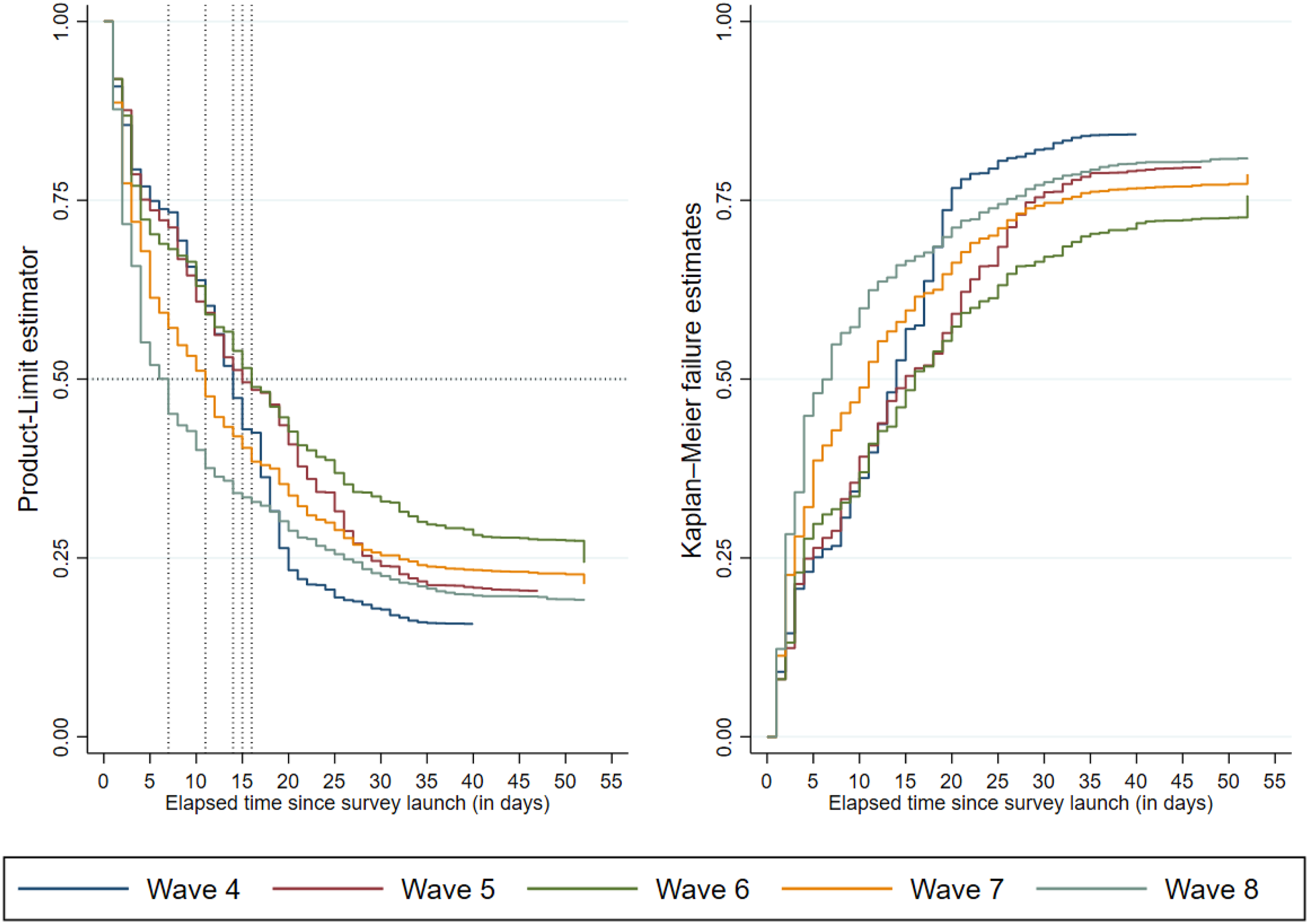

Overall, we demonstrate that the quantiles of the empirical response time distribution seem to be adequate for describing the timing of survey participation. If the first quarter is used for measuring the increased response speed across panel waves, it is found that it took five days after the invitation till 25 per cent of the invitees had responded. This parameter decreased to four days in Wave 6, then to three days in Wave 7 and finally to two days in Wave 8.

If one uses this parameter for the classification of ‘early’, ‘intermediate’ and ‘late’ respondents, it becomes obvious that the tempo of responses for each of these groups is different for each of the waves. While in Wave 4, for example, the invitees could be defined as ‘early’ respondents when they responded within four days after being invited to take part in the survey, and they were classified as ‘intermediate’ respondents if they responded within 15 days, for Wave 8, the class levels are much lower: they are ‘early’ respondents if they respond within two days, and the remaining non-respondents are ‘intermediate’ respondents if their response occurs before the end of the first week; the respondents in the remaining risk sample after a week are ‘late’ respondents. It should be noticed that the definition of an ‘intermediate’ respondent in Wave 8 is almost consistent with the definition of an ‘early’ respondent in Wave 4. This finding demonstrates that the definition of such response groups is rather confusing. The use of quartiles, however, makes it possible to compare the timing of response across surveys without any reference to determined value ranges of the response.

The finding is replicated by considering the competing risks regarding the choice between different survey modes across the fieldwork period and across panel waves. For this purpose, the CIFs are estimated (see Figure 2). In the left-hand panel, it is shown that for the online mode the response rate increased across panel waves. While the median values of the timing of the response in this initial mode are the same as those for each of the survey modes, the response rates are different. The response rate increased continuously across the waves, from 46 per cent in Wave 4 to 76 per cent in Wave 8. At the same time, the response rate in the telephone mode (right-hand panel) decreased from 52 per cent in Wave 4 to 15 per cent in Wave 8. The median value estimated by the traditional survival analysis is 10 days after the first offer of the CATI mode in Wave 4 (i.e. 22 days after the survey launch), 15 days in Wave 5 and 27 days in Wave 6. For waves 7 and 8, it is not possible to calculate the median value. In these waves, most of the invitees responded in the initial mode, while the non-respondents to whom the alternative mode had been offered were less willing to respond in time.

Figure 2.

CIF – comparison between survey modes across panel waves.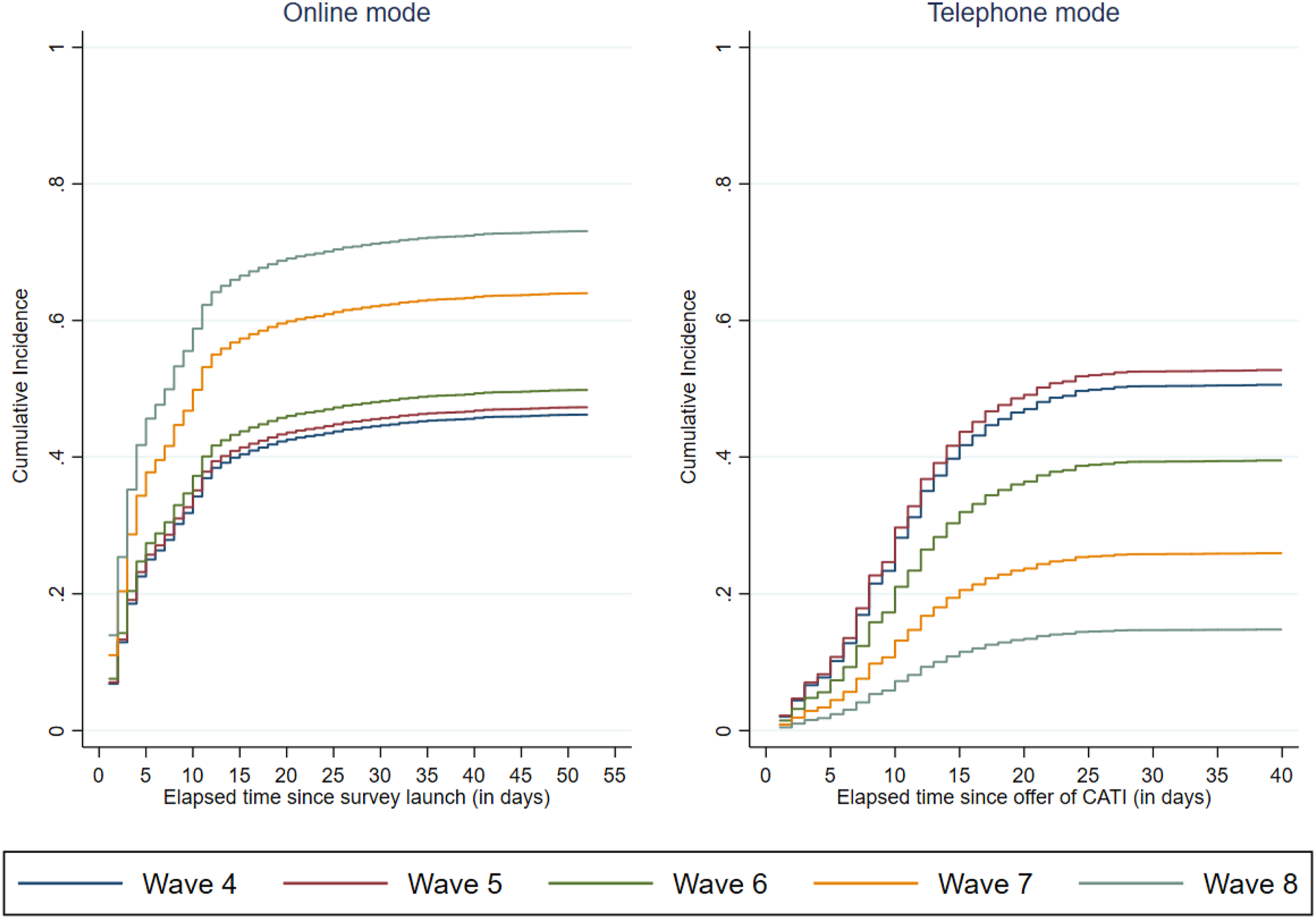

In sum, the findings confirm our conclusion that the classification of response groups is not useful. However, the positive message is that the use of non-parametric procedures and related univariate parameters, such as quartiles, provides descriptions of the timing of survey participation and the development of the overall response rate across the time that elapses after survey launch.

Dynamics of Period-Specific Survey Participation

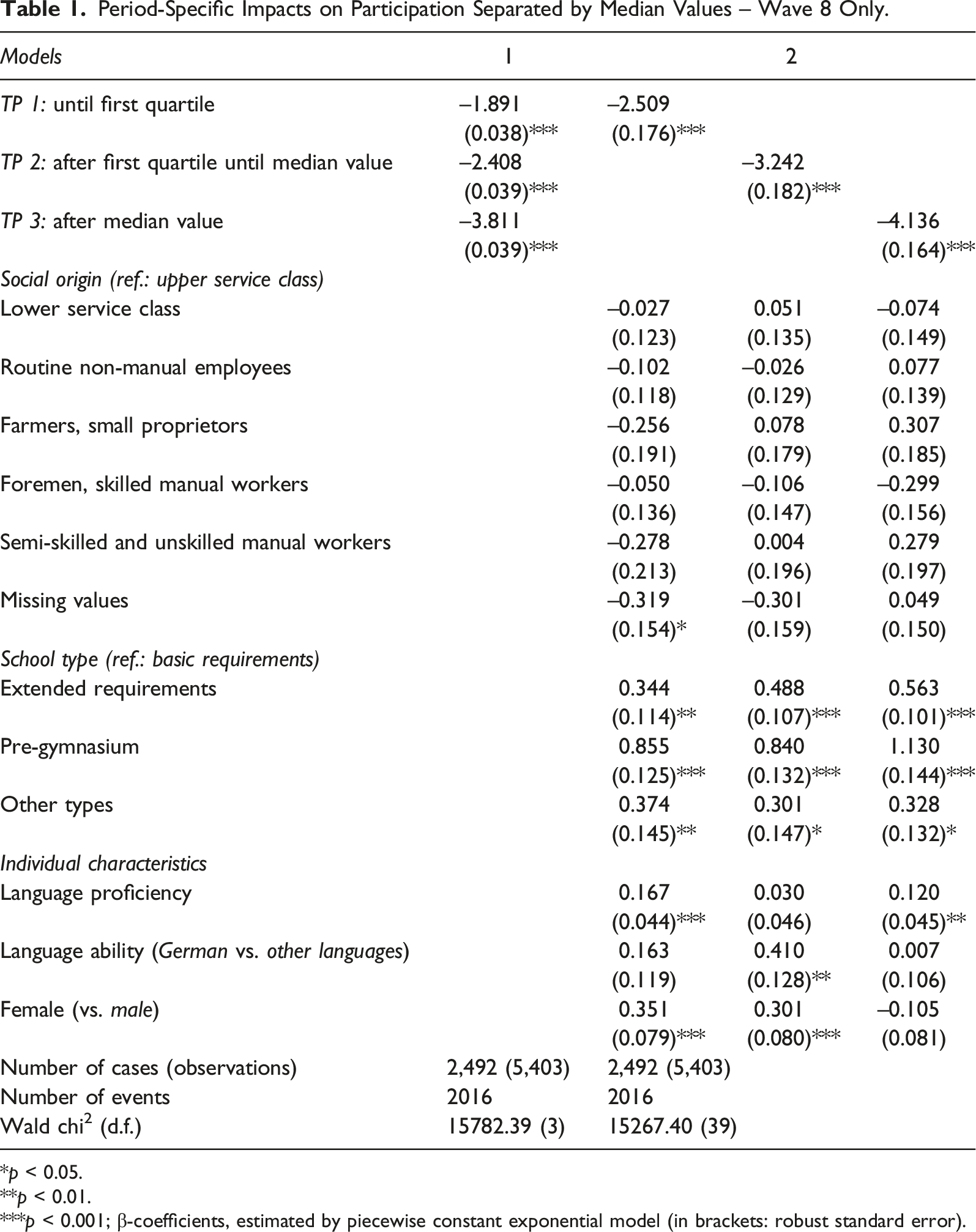
Based on the previous description of the timing of survey participation, the calculated quartiles are used to distinguish different stages of the fieldwork period. By employing the piecewise constant exponential model, it is possible to reveal whether the delays in survey response differ between stages of the fieldwork period and by the panelists’ characteristics surviving in these stages. Dividing the fieldwork period into three sub-periods, with the first quartile and the median being the threshold values for the episode splitting, yields interesting results (Table 1). This procedure is used for the last wave only, for the sake of demonstration.

Table 1.

Period-Specific Impacts on Participation Separated by Median Values – Wave 8 Only.

Models	1	2
TP 1: until first quartile	–1.891	–2.509
	(0.038)***	(0.176)***
TP 2: after first quartile until median value	–2.408		–3.242
	(0.039)***		(0.182)***
TP 3: after median value	–3.811			–4.136
	(0.039)***			(0.164)***
Social origin (ref.: upper service class)
Lower service class		–0.027	0.051	–0.074
		(0.123)	(0.135)	(0.149)
Routine non-manual employees		–0.102	–0.026	0.077
		(0.118)	(0.129)	(0.139)
Farmers, small proprietors		–0.256	0.078	0.307
		(0.191)	(0.179)	(0.185)
Foremen, skilled manual workers		–0.050	–0.106	–0.299
		(0.136)	(0.147)	(0.156)
Semi-skilled and unskilled manual workers		–0.278	0.004	0.279
		(0.213)	(0.196)	(0.197)
Missing values		–0.319	–0.301	0.049
		(0.154)*	(0.159)	(0.150)
School type (ref.: basic requirements)
Extended requirements		0.344	0.488	0.563
		(0.114)**	(0.107)***	(0.101)***
Pre-gymnasium		0.855	0.840	1.130
		(0.125)***	(0.132)***	(0.144)***
Other types		0.374	0.301	0.328
		(0.145)**	(0.147)*	(0.132)*
Individual characteristics
Language proficiency		0.167	0.030	0.120
		(0.044)***	(0.046)	(0.045)**
Language ability (German vs. other languages)		0.163	0.410	0.007
		(0.119)	(0.128)**	(0.106)
Female (vs. male)		0.351	0.301	–0.105
		(0.079)***	(0.080)***	(0.081)
Number of cases (observations)	2,492 (5,403)	2,492 (5,403)
Number of events	2016	2016
Wald chi² (d.f.)	15782.39 (3)	15267.40 (39)

*p < 0.05.

**p < 0.01.

***p < 0.001; β-coefficients, estimated by piecewise constant exponential model (in brackets: robust standard error).

The first sub-period lasts two days, and the second sub-period lasts seven days. The third sub-period consists of the rest of the fieldwork period. By considering three points in time (TP), it becomes obvious that the likelihood of survey participation decreases across the fieldwork period (models 1 and 2).

Furthermore, it is revealed that the patterns of socially selective participation are somewhat different for the different stages of the fielding. First of all, there is no selectivity of participation in terms of social origin. Second, however, the effect of panelists’ education increases across the sub-periods in favour of well-educated individuals compared to panelists with a lower educational level. In particular, this is true for panelists who were enrolled in a pre-gymnasium and a secondary school with extended requirements. This type of selectivity might explain the education bias in the realized survey. Third, panelists with pronounced language proficiency are more likely to take part in the survey, while language ability provides no systematic effect across each of the sub-periods. However, until the median value of the delay in survey response, it is found that individuals with a strong ability in the German language are more likely to respond than their counterparts. Fourth, and finally, it is revealed that women are more likely to respond immediately after survey launch or in the first stages of the fieldwork period, than the male panelists. This persistent gender effect should be subjected to detailed analysis in the future (Becker, 2021).

In sum, this analysis demonstrates again that it is interesting to analyze different phases of fieldwork, instead of classifying different response groups. These stages provide information about how likely is it for invitees to catch up for their delayed response.

Ways of Accelerating Survey Response Speed

How can an acceleration of the survey response speed, in terms of a shift in the timing of response to earlier stages of the fieldwork, be explained? What are the consequences of this development within a panel with a sequential mixed-mode design? Incentives of an increasing value across panel waves might be expected to increase the response speed across the waves, while the response rates remain rather constant. While in the fourth wave, half of the invitees received a voucher (worth 10 Swiss Francs) and the other half received no incentive, each of the panelists received a voucher in Wave 5, an engraved ballpoint pen in Wave 6 and cash (a 10 Swiss Francs banknote) in Wave 8.

Therefore, it is tested whether the change in the unconditional incentives, from in-kind to prepaid money, resulted in different response patterns across survey modes and panel waves. For this purpose, competing-risk models are estimated (Table 2). By controlling for previous participation and choice of survey mode, it is found that the receipt of cash in waves 7 and 8 had the largest impact on the timing of survey participation and, as a consequence, on the choice of survey mode. Compared to Wave 4, cash in Wave 8 increased the propensity to respond by about

[(\exp (1.24) - 1) ∙ 100 % =]

246 per cent, while the propensity to participate in the CATI mode decreased by about

[(\exp (- 1.192) - 1) ∙ 100 % =]

70 per cent.

Table 2.

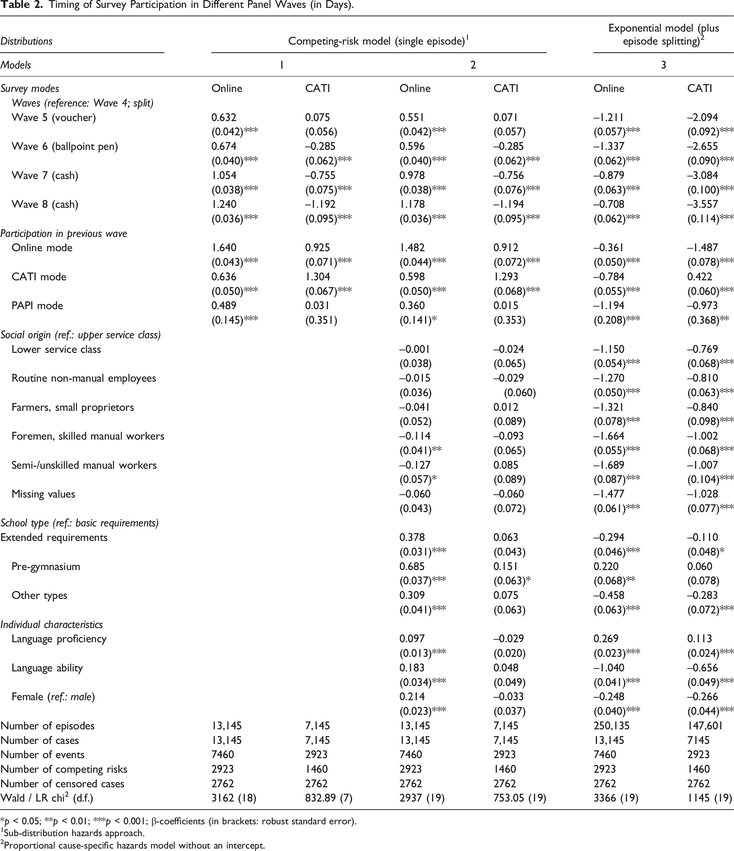
Timing of Survey Participation in Different Panel Waves (in Days).

Distributions	Competing-risk model (single episode)¹				Exponential model (plus episode splitting)²
Models	1		2		3
Survey modes	Online	CATI	Online	CATI	Online	CATI
Waves (reference: Wave 4; split)
Wave 5 (voucher)	0.632	0.075	0.551	0.071	–1.211	–2.094
	(0.042)***	(0.056)	(0.042)***	(0.057)	(0.057)***	(0.092)***
Wave 6 (ballpoint pen)	0.674	–0.285	0.596	–0.285	–1.337	–2.655
	(0.040)***	(0.062)***	(0.040)***	(0.062)***	(0.062)***	(0.090)***
Wave 7 (cash)	1.054	–0.755	0.978	–0.756	–0.879	–3.084
	(0.038)***	(0.075)***	(0.038)***	(0.076)***	(0.063)***	(0.100)***
Wave 8 (cash)	1.240	–1.192	1.178	–1.194	–0.708	–3.557
	(0.036)***	(0.095)***	(0.036)***	(0.095)***	(0.062)***	(0.114)***
Participation in previous wave
Online mode	1.640	0.925	1.482	0.912	–0.361	–1.487
	(0.043)***	(0.071)***	(0.044)***	(0.072)***	(0.050)***	(0.078)***
CATI mode	0.636	1.304	0.598	1.293	–0.784	0.422
	(0.050)***	(0.067)***	(0.050)***	(0.068)***	(0.055)***	(0.060)***
PAPI mode	0.489	0.031	0.360	0.015	–1.194	–0.973
	(0.145)***	(0.351)	(0.141)*	(0.353)	(0.208)***	(0.368)**
Social origin (ref.: upper service class)
Lower service class			–0.001	–0.024	–1.150	–0.769
			(0.038)	(0.065)	(0.054)***	(0.068)***
Routine non-manual employees			–0.015	–0.029	–1.270	–0.810
			(0.036)	(0.060)	(0.050)***	(0.063)***
Farmers, small proprietors			–0.041	0.012	–1.321	–0.840
			(0.052)	(0.089)	(0.078)***	(0.098)***
Foremen, skilled manual workers			–0.114	–0.093	–1.664	–1.002
			(0.041)**	(0.065)	(0.055)***	(0.068)***
Semi-/unskilled manual workers			–0.127	0.085	–1.689	–1.007
			(0.057)*	(0.089)	(0.087)***	(0.104)***
Missing values			–0.060	–0.060	–1.477	–1.028
			(0.043)	(0.072)	(0.061)***	(0.077)***
School type (ref.: basic requirements)
Extended requirements			0.378	0.063	–0.294	–0.110
			(0.031)***	(0.043)	(0.046)***	(0.048)*
Pre-gymnasium			0.685	0.151	0.220	0.060
			(0.037)***	(0.063)*	(0.068)**	(0.078)
Other types			0.309	0.075	–0.458	–0.283
			(0.041)***	(0.063)	(0.063)***	(0.072)***
Individual characteristics
Language proficiency			0.097	–0.029	0.269	0.113
			(0.013)***	(0.020)	(0.023)***	(0.024)***
Language ability			0.183	0.048	–1.040	–0.656
			(0.034)***	(0.049)	(0.041)***	(0.049)***
Female (ref.: male)			0.214	–0.033	–0.248	–0.266
			(0.023)***	(0.037)	(0.040)***	(0.044)***
Number of episodes	13,145	7,145	13,145	7,145	250,135	147,601
Number of cases	13,145	7,145	13,145	7,145	13,145	7145
Number of events	7460	2923	7460	2923	7460	2923
Number of competing risks	2923	1460	2923	1460	2923	1460
Number of censored cases	2762	2762	2762	2762	2762	2762
Wald / LR chi² (d.f.)	3162 (18)	832.89 (7)	2937 (19)	753.05 (19)	3366 (19)	1145 (19)

*p < 0.05; **p < 0.01; ***p < 0.001; β-coefficients (in brackets: robust standard error).

¹Sub-distribution hazards approach.

²Proportional cause-specific hazards model without an intercept.

Even in-kind gifts, such as a voucher or a ballpoint pen, result in a decreased delay in survey response. They also lead to an increased response in the initial survey mode. The positive impact of participation in the previous panel wave and previously chosen survey mode on the timing of the survey response confirms this conclusion. On the one hand, the reproduction of mode choice probably indicates panelists’ mode preference. Panelists who previously took part in the online mode mostly choose the same mode in the next wave. This is also true for the preference for the CATI mode, but there are quantitative differences in favour to the online mode. On the other hand, it is also found that panelists switch to another mode in the next wave. However, the trade-off is in favour of the online mode. These findings are valid even if one considers the panelists’ characteristics (model 2).

By utilizing the proportional cause-specific hazards model (without an intercept), it is possible to quantify the impact of time-varying covariates on the individuals’ timing of their response. While for panelists who received cash in Wave 8, an average delay of $[1 / \exp (- 0.708) =]$ 2 days is expected in regard to responding in the online mode, the average delay for a response in the initial mode in Wave 8, based on the voucher, is $[1 / \exp (- 1.211) =]$ 3.8 days. For panelists who completed the online questionnaire in the previous wave, the expected delay in the current wave is about $[1 / \exp (- 0.361) =]$ 1.4 days, and it is about 2 days for those who responded previously in the CATI mode, while it is more than 3 days for those who responded previously in the PAPI mode.

For panelists invited to participate in Wave 8 and who took part in the online mode previously, one could expect an average delay of $[1 / \exp (- 0.708 + - 0.361) =]$ 2.9 days, while for target persons in Wave 6 we expect an average delay of more than $[1 / \exp (- 1.337 + - 0.784) =]$ 8 days, provided that they took part in the CATI mode in the previous Wave 5. If one considers the characteristics of target persons, it is possible to estimate their average delay until survey response. In our view, the categorization of the respondents into ‘early’ or ‘late’ respondents becomes rather obsolete.

Furthermore, it is possible to evaluate another effect of fieldwork period management on the timing of survey participation. It is assumed that the digital follow-up invitation sent additionally after the prior invitation letter has been sent by regular postage mail, as well as the digital reminders, ‘caused’ an increase in survey participation and stopped the target persons who received them delaying their response to a future point in time.

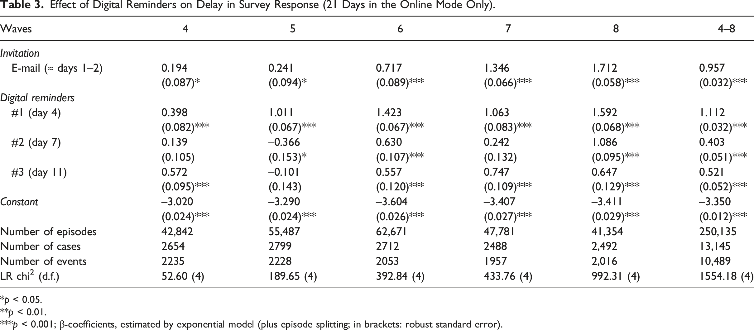
This assumption is confirmed by multivariate estimations limited to the first three weeks of fieldwork and to the online mode (Table 3). The digital follow-up invitation, as well as the reminders sent by e-mail, encourages invitees’ survey participation, leading to decreased delay in responding to the survey and increased likelihood of participating in the survey. The impact of the digital follow-up invitation on the response speed increases across the waves.

Table 3.

Effect of Digital Reminders on Delay in Survey Response (21 Days in the Online Mode Only).

Waves	4	5	6	7	8	4–8
Invitation
E-mail (≈ days 1–2)	0.194	0.241	0.717	1.346	1.712	0.957
	(0.087)*	(0.094)*	(0.089)***	(0.066)***	(0.058)***	(0.032)***
Digital reminders
#1 (day 4)	0.398	1.011	1.423	1.063	1.592	1.112
	(0.082)***	(0.067)***	(0.067)***	(0.083)***	(0.068)***	(0.032)***
#2 (day 7)	0.139	–0.366	0.630	0.242	1.086	0.403
	(0.105)	(0.153)*	(0.107)***	(0.132)	(0.095)***	(0.051)***
#3 (day 11)	0.572	–0.101	0.557	0.747	0.647	0.521
	(0.095)***	(0.143)	(0.120)***	(0.109)***	(0.129)***	(0.052)***
Constant	–3.020	–3.290	–3.604	–3.407	–3.411	–3.350
	(0.024)***	(0.024)***	(0.026)***	(0.027)***	(0.029)***	(0.012)***
Number of episodes	42,842	55,487	62,671	47,781	41,354	250,135
Number of cases	2654	2799	2712	2488	2,492	13,145
Number of events	2235	2228	2053	1957	2,016	10,489
LR chi² (d.f.)	52.60 (4)	189.65 (4)	392.84 (4)	433.76 (4)	992.31 (4)	1554.18 (4)

*p < 0.05.

**p < 0.01.

***p < 0.001; β-coefficients, estimated by exponential model (plus episode splitting; in brackets: robust standard error).

This development is probably also based on the effect of different prepaid incentives across the waves. Overall, this feature of survey management is useful for enhancing panelists’ participation in terms of the timing of their response. For 1 to 3 days, on the one hand, the first reminder enhanced the response rate by between 49 per cent (in Wave 4) and 391 per cent (Wave 8).

Summary and conclusion

In conjunction with research on the timing of survey participation and the development of response rates across a fieldwork period, the aim of this contribution is twofold. On the one hand, it demonstrates that different classifications of invitees into ‘early’, ‘intermediate’ and ‘late’ respondents are without any epistemological or methodological foundation. On the other hand, both dimensions – the timing of survey participation as a stochastic process of individuals’ response and the development of the response rate as its time-related consequence – are investigated by analyzing paradata of the fieldwork period of an established panel study. The paradata are linked with the characteristics of surveys and eligible panelists. For the description and multivariate estimations of response speed across sequentially mixed modes and panel waves, the techniques and procedures of event history analysis are utilized to demonstrate an alternative way to analyze the time dimensions of target persons’ response behaviour.

Different procedures of non-parametric survival analysis and parametric models of event history contribute theoretically, methodologically and statistically adequate alternatives to answer the question: How long does it take for a number of individuals to respond to the invitation to participate in a survey? These procedures deliver precise information on the timing of survey participation which is more useful than the categorization of ‘early’, ‘intermediate’ and ‘late’ respondents. They also provide information on the trajectory of responses and non-responses across the time that elapses after the survey launch. For the analysis on the impacts of various factors on invitees’ timing of their survey participation, it is possible to consider individuals’ resources and abilities, as well as features of the survey management. It becomes obvious that important information is missing which is necessary to understand the survey participation completely. It is difficult to collect this information, as it would involve interviewing non-respondents or observing the reasons behind their survey behaviour. Mostly important are events and processes occurring across the running fieldwork period – for example, time-varying opportunities of invitees to take part in the survey or changes in their attitudes towards the survey and their evaluation of the costs and benefits of participation. Finally, answers to the third question about the practical implications of procedures in the fieldwork are found. Prepaid incentives or follow-up reminders, to give an example, are helpful in regard to significantly boosting the response rate and the speed of return. It is also found that the effect of such strategies fades across time.

As a by-product of these analyses, it became evident that it is not empirically useful to categorize different types of ‘early’ or ‘late’ respondents. First, individuals’ survey response is a stochastic event that results in different tempi and in different social structures of response across panel waves. Second, there is a change in the sample, in terms of size and social structure; therefore, the arbitrary definition of such categories is not useful (Gummer & Struminskaya, 2020). Third, the theoretical surplus value of such a category scheme is unclear. Finally, for the survey methodology, it is of interest how we can realize a survey in an efficient and less selective way. Categorizing types of interviewees or controlling for their psychological traits does not help us to understand the time-varying decision to participate or the outcome in a survey or among surveys in the context of a panel study (Groves et al., 1992). In order to achieve a rather limited fieldwork period in order to minimize the costs and thus reduce the project budget, it might be more important to reveal which treatments – such as incentives, reminders or other events happening at different points in time during the fieldwork – are significant for the timing of survey participation. Which of these increase the participation rate in a mixed-mode probability-based panel survey? For example, the significant impact of prepaid incentives and digital reminders on panelists’ timing of their response in different waves was revealed by non-parametric and parametric procedures based on adequate techniques of event history analysis. In sum, this contribution also calls for dynamic longitudinal analyses of response behaviour, instead of a rather useless classification of response groups in the manner of comparative-static approach.

Taking a dynamic view in a longitudinal design, evidence-based practical implications become empirically clearer than in a comparative-static design. Evidence-based advice regarding the length of the fieldwork period until the cutoff of the data collection and other dimensions of survey management are provided by such data and statistical analysis (Chebat & Cohen, 1993). Because the timing of survey participation ‘has cost implications, slow response tends to increase the extensiveness of follow-up efforts and therefore the cost of study’ (Houston & Ford, 1976, p. 397). Thus, it is clear that the timing of survey participation is a function of the time that elapses after mailing the invitation letter, which is tailored to the target persons and encloses an incentive, and the reminders. In addition, we now know when panelists endowed with different resources and abilities start responding to the invitation to take part in a survey. Furthermore, time- and event-related analysis shows why a mixed-mode design is a rational approach when dealing with procrastinating target persons, to motivate them to respond.

With the help of in-depth knowledge on such stochastic processes, it might be possible to plan and manage fieldwork in a rational way, as opposed to applying an apparently plausible patchwork, such as is often observed in survey methodology. What remains a problem is that we still do not know how, why and when special arrangements work in the field. However, possession of this evidence-based knowledge might save time and costs for researchers, as well as for the target persons of their research (Houston & Ford, 1976). It would also prevent a hasty shortening of the fieldwork period since this would increase the negative consequences in terms of the social selective response rate and the selectivity of surviving panel samples. However, based on such longitudinal designs and dynamic analysis, we would be able to shorten the fieldwork period without adversely affecting the quality of the data produced (Sigman et al., 2014). This would be enabled by direct testing of theories seeking to explain survey participation and its timing.

However, there are limitations to our arguments. First, as none of the theories on survey participation have really been tested empirically, it is difficult to realize the ideas discussed in this contribution. Collecting time-varying information on the processes and mechanisms behind target persons’ response behaviour is a huge challenge. In general, it would involve interviewing non-respondents. Second, for the empirical demonstration, this involved a special population of youths in a single birth cohort (born around 1997) living in German-speaking cantons of Switzerland. Therefore, it may be true that the empirical results are not generally valid for other populations. However, this does not contradict the ‘philosophy’ of the call for dynamic longitudinal analysis of response behaviour in an event-oriented design, instead of cross-sectional analysis in a comparative-static design. The results regarding the effect of incentives and reminders are in favour of this argument since they are in line with the findings for other target populations. In sum, there is a need to replicate the analysis for other populations and different types of survey modes not considered in this contribution. Third, it is difficult to disentangle different causes of response speed and response rate. On the one hand, this is a theoretical and methodological problem. On the other hand, this leads to a need for different longitudinal designs in future, which are well-constructed, in order to reveal causal impacts on the timing of survey participation.

Footnotes

Acknowledgements

For helpful comments and discussions on earlier versions of this manuscript, I wish like to thank Peter Blossfeld, Richard Nennstiel and Thorsten Schneider. The author is responsible for all remaining inadequacies.

Declaration of Conflicting Interests

The author(s) declared no potential conflicts of interest with respect to the research, authorship, and/or publication of this article.

Funding

The author(s) disclosed receipt of the following financial support for the research, authorship, and/or publication. The DAB panel study is substantially financed by the State Secretariat for Education, Research and Innovation (SERI). The interpretations and conclusions are those of the authors and do not necessarily represent the views of the SERI.

Data Availability Statement

The data for the first nine waves of the panel study are available as Scientific Use Files at FORS in Lausanne (DOI: https://doi.org/10.48573/dqgk-ja58) and can be found in the SWISSUbase online catalogue under the reference number 10773 (https://www.swissubase.ch/en/catalogue/studies/10773/latest/datasets/946/2519/overview). The Stata syntax used for this contribution is available from the author. .

Notes

Author Biography

Rolf Becker is Full Professor and Chair of the Department of Sociology of Education at the University of Bern. His research interests include life course research, labour market and mobility research, sociology of education, social stratification and mobility as well as methods of empirical social research and longitudinal data analysis. He is head of the panel study “Determinants of Educational Choice and Vocational Training Opportunities in Switzerland” (DAB), co-applicant of the panel study “Transition from education to employment” (TREE), and member of the board of ICER (Interfaculty Centre of Educational Research). His scientific work has been published in European Sociological Review, Rationality & Society, Quality & Quantity, Survey Research Methods, Longitudinal and Life Course Studies, MDA (Methods-Data-Analyses), Social Science Research, Journal of Choice Modelling, and other academic journals.

References

Aalen

O. O.

Ørnulf

Gjessing

H. K.

(2008). Survival and event history analysis. Springer.

AAPOR (The American Association for Public Opinion Research) (2016). Standard definitions: Final dispositions of case codes and outcome rates for surveys (9th edition). AAPOR.

Austin

P. C.

Fine

J. P.

(2017). Practical recommendations for reporting Fine‐Gray Model Analyses for competing risk data. Statistics in Medicine, 36(27), 4391–4400. https://doi.org/10.1002/sim.7501

Becker

(2021). Gender and survey participation. an event history analysis of the gender effects of survey participation in a probability-based multi-wave panel study with a sequential mixed-mode design. Methods – Data – Analyses, 16(1), 1–29. https://doi.org/10.12758/mda.2021.08

Becker

Glauser

(2018). Are prepaid monetary incentives sufficient for reducing panel attrition and optimizing the response rate? An experiment in the context of a multi-wave panel with a sequential mixed-mode design. Bulletin of Sociological Methodology, 137(1), 74–95. https://doi.org/10.1177/0759106318762456

Becker

Glauser

Möser

(2020). Determinants of educational choice and vocational training opportunities in Switzerland – empirical analyses with longitudinal data from the DAB panel study. In McElvany

Holtappels

H.-G.

Lauermann

Edele

Ohle-Peters

(Eds.), Against the odds – (In)Equity in education and educational systems (pp. 125–143). Waxmann.

Becker

Möser

Glauser

(2019). Cash vs. vouchers vs. gifts in web surveys of a mature panel study––main effects in a long-term incentives experiment across three panel waves. Social Science Research, 81(July), 221–234. https://doi.org/10.1016/j.ssresearch.2019.02.008

Blossfeld

H.-P.

(1996). Macro-sociology, rational choice theory and time. A theoretical perspective on the empirical analysis of social processes. European Sociological Review, 12(2), 181–206. https://doi.org/10.1093/oxfordjournals.esr.a018185

Blossfeld

H.-P.

Rohwer

(1997). Causal inference, time and observation plans in the social sciences. Quality and Quantity, 31(November), 361–384. https://doi.org/10.1023/A:1004289932598

10.

Blossfeld

H.-P.

Rohwer

Schneider

(2019). Event history analysis with Stata. Routledge.

11.

Boek

W. E.

(1990). A comparison of early with late respondents to a mailed questionnaire. Journal of the Washington Academy of Sciences, 80(4), 153–160. https://www.jstor.org/stable/24536119

12.

Callegaro

Baker

Bethlehem

Göritz

Krosnick

J. A.

Lavrakas

P. J.

(Eds.), (2014). Online panel research: A data quality perspective. John Wiley & Sons.

13.

Chebat

J.-C.

Cohen

(1993). Response speed in mail surveys: Beware of shortcuts. Marketing Research, 5(1), 20–25. https://search.ebscohost.com/login.aspx?direct=true&profile=ehost&scope=site&authtype=crawler&jrnl=10408460&AN=9602160676&h=AZ3MVucUMWMqYm9FlotTeC%2F%2B7e6lKevjQH7ZPcmSdbgtm8xuyUgKobhIyeSoMVvbUy4O9jwe0zjqSmUlOrvHMQ%3D%3D&crl=c

14.

Chen

Wei

Syme

P. D.

(2003). Comparison of early and delayed respondents to a postal health survey: A questionnaire study of personality traits and neuropsychological symptoms. European Journal of Epidemiology, 18(3), 195–202. https://doi.org/10.1023/A:1023393231234

15.

de Leeuw

E. D.

(2018). Mixed-Mode: Past, present, and future. Survey Research Methods, 12(2), 75–89. https://doi.org/10.18148/srm/2018.v12i2.7402

16.

Dillman

D. A.

Phelps

Tortora

Swift

Kohrell

Berck

Messer

B. L.

(2009). Response rate and measurement differences in mixed-mode surveys using mail, telephone, interactive voice response (IVR) and the internet. Social Science Research, 38(1), 1–18. https://doi.org/10.1016/j.ssresearch.2008.03.007

17.

Durrant

G. B.

D’Arrigo

Müller

(2013). Modeling call record data: Examples from cross-sectional and longitudinal surveys. In Kreuter

(Ed.), Improving surveys with paradata: Analytic uses of process information (pp. 281–308). John Wiley & Sons.

18.

Durrant

G. B.

D’Arrigo

Steele

(2013). Analysing interviewer call record data by using a multilevel time event history modelling approach. Journal of the Royal Statistical Society, 176(1), 251–269. https://doi.org/10.1111/j.1467-985X.2012.01073.x

19.

Erikson

Goldthorpe

J. H.

(1992). The constant flux. Clarendon Press.

20.

Faria

A. J.

Dickinson

J. R.

(1992). Mail survey response, speed, and cost. Industrial Marketing Management, 21(1), 51–60. https://doi.org/10.1016/0019-8501(92)90033-P

21.

Fine

J. P.

Gray

R. J.

(1999). A Proportional Hazards Model for the subdistribution of a competing risk. Journal of the American Statistical Association, 94(446), 496–509.

22.

Göritz

A. S.

(2014). Determinants of the starting rate and the completion rate in online panel studies. In Callegaro

Baker

Bethlehem

Göritz

A. S.

Krosnick

J. A.

Lavrakas

P. J.

(Eds.), Online panel research: A data quality perspective (pp. 154–170). John Wiley & Sons.

23.

Göritz

A. S.

(2015). Incentive effects. In Engel

Jann

Lynn

Scherpenzeel

Sturgies

(Eds.), Improving survey methods (pp. 339–350). Routledge.

24.

Göritz

A. S.

Stieger

(2009). The impact of the field time on response, retention, and response completeness in list-based Web surveys. International Journal of Human Computer Studies, 67(4), 342–348. https://doi.org/10.1016/j.ijhcs.2008.10.002

25.

Green

K. E.

(2014). Reluctant respondents. Differences between early, late and nonresponders to a mail survey. Journal of Experimental Education, 59(3), 268–276. https://doi.org/10.1080/00220973.1991.10806566

26.

Groves

R. M.

Cialdini

R. B.

Couper

M. P.

(1992). Understanding the decision to participate in a survey. Public Opinion Quarterly, 56(4), 475–495. https://doi.org/10.1086/269338

27.

Groves

R. M.

Couper

M. P.

(1998). Nonresponse in household interview surveys. John Wiley & Sons.

28.

Gummer

Struminskaya

(2020). Early and late participation during the field period: Response timing in a mixed-mode probability-based panel survey. Sociological Methods & Research, 49(2), 1–24. https://doi.org/10.1177/0049124120914921

29.

Houston

M. J.

Ford

N. M.

(1976). Broadening the scope of methodological research on mail surveys. Journal of Marketing Research, 13(4), 397–403. https://doi.org/10.1177/002224377601300410

30.

Huxley

S. J.

(1980). Predicting response speed in mail surveys. Journal of Marketing Research, 17(1), 63–68. https://doi.org/10.1177/002224378001700108

31.

Kalbfleisch

J. D.

Prentice

R. L.

(2002). The statistical analysis of failure time data (2nd edition). Wiley & Sons.

32.

Klingwort

Buelens

B. v.

Schnell

(2018). Early versus late respondents in web surveys: Evidence from a national health survey. Statistical Journal of the IAOS, 34(3), 461–471. https://doi.org/10.3233/SJI-170421

33.

Kreuter

(2015). The use of paradata. In Engel

Jann

Lynn

Scherpenzeel

Sturgis

(Eds.), Improving survey methods (pp. 303–318). Routledge.

34.

Kreuter

Müller

Trappmann

(2014). A note on mechanisms leading to lower data quality of late or reluctant respondents. Sociological Methods & Research, 43(3), 452–464. https://doi.org/10.1177/0049124113508094

35.

Lahaut

V. M.

Jansen

H. A. M.

Mheen

D. v. d.

Garretsen

H. F. L.

Verdurmen

J. E. E.

Dijk

A. v.

(2002). Estimating non-response bias in A survey on alcohol consumption: Comparison of response waves. Alcohol & Alcoholism, 38(2), 128–134. https://doi.org/10.1093/alcalc/agg044

36.

Lambert

P. C.

(2017). The estimation and modeling of cause-specific cumulative incidence functions using time-dependent weights. Stata Journal, 17(1), 181–207. https://doi.org/10.1177/1536867X1701700110

37.

Lipps

Herzing

J. M. E.

Pekari

Stähli

M. E.

Pollien

Riedo

Reveilhac

(2019). Incentives in surveys. FORS guide No. 08. FORS.

38.

Lugtig

(2014). Panel attrition: Separating stayers, fast attriters, gradual attriters, and lurkers. Sociological Methods & Research, 43(4), 699–723. https://doi.org/10.1177/0049124113520305

39.

Lunn

McNeil

(1995). Applying cox regression to competing risks. Biometrics, 51(2), 524–532. https://www.jstor.org/stable/2532940

40.

Lynn

(Eds.), (2009). Methodology of longitudinal surveys. Wiley.

41.

Lynn

(2020). Evaluating push-to-web methodology for mixed-mode surveys using address-based samples. Survey Research Methods, 14(1), 19–30. https://doi.org/10.18148/srm/2020.v14i1.7591

42.

Noordzij

Leffondré

Stralen

K. J. v.

Zocali

Dekker

F. W.

Jager

K. J.

(2013). When do we need competing risks methods for survival analysis in nephrology? Nephrology Dialysis Transplantation, 28(11), 2670–2677. https://doi.org/10.1093/ndt/gft355

43.

Novo

Hammarström

Janlert

(1999). Does low willingness to respond introduce a bias? Results from a socio-epidemiological study among young men and women. International Journal of Social Welfare, 8(2), 155–163. https://doi.org/10.1111/1468-2397.00076

44.

Olowokure

Caswell

Duggal

H. V.

(2004). Response patterns to a postal survey using a cervical screening register as the sampling frame. Public Health, 118(7), 508–512. https://doi.org/10.1016/j.puhe.2003.12.013

45.

Rao

Pennington

(2013). Should the third reminder be sent? The role of survey response timing on web survey results. International Journal of Market Research, 55(5), 651–674. https://doi.org/10.2501/IJMR-2013-056

46.

Sauermann

Roach

(2013). Increasing web survey response rates in innovation research: An experimental study of static and dynamic contact design features. Research Policy, 42(1), 273–286. https://doi.org/10.1016/j.respol.2012.05.003

47.

Schuster

N. A.

Hoogendijka

E. O.

Koka

A. A. L.

Twiska

J. W. R.

Heymansa

M. W.

(2020). Ignoring competing events in the analysis of survival data may lead to biased results: A nonmathematical illustration of competing risk analysis. Journal of Clinical Epidemiology, 122(1), 42–48. https://doi.org/10.1016/j.jclinepi.2020.03.004

48.

Sigman

Lewis

Yount

N. D.

Lee

(2014). Does the length of fielding period matter? Examining response scores of early versus late responders. Journal of Official Statistics, 30(4), 651–674.

49.

Singer

(2006). Introduction: Nonresponse bias in household surveys. Public Opinion Quarterly, 70(5), 637–645. https://doi.org/10.1093/poq/nfl034

50.

Singer

(2011). Toward a benefit–cost theory of survey participation: evidence, further tests, and implication. Journal of Official Statistics, 27(2), 379–393.

51.

Singer

(2013). The use and effects of incentives in surveys. The Annals of the American Academy of Political and Social Science, 645(1), 112–141. https://doi.org/10.1177/0002716212458082

52.

Studer

Baggio

Mohler-Kuo

Dermota

Gaume

Bertholet

Daeppen

J.-B.

Gmel

(2013). Examining non-response bias in substance use research – are late respondents proxies for non-respondents? Drug and Alcohol Dependence, 132(1–2), 316–323. https://doi.org/10.1016/j.drugalcdep.2013.02.029

53.

Tourangeau

Conrad

F. G.

Couper

M. P.

(2013). The science of web surveys. Oxford University Press.

54.

Truell

A. D.

Bartlett

J. E.

II Alexander

M. W.

(2002). Response rate, speed, and completeness: A comparison of internet-based and mail surveys. Behavior Research Methods, Instruments & Computers, 34(1), 46–49. https://doi.org/10.3758/BF03195422

55.

Van Mol

(2017). Improving web survey efficiency: The impact of an extra reminder and reminder content on web survey response. International Journal of Social Research Methodology, 20(4), 317–327. https://doi.org/10.1080/13645579.2016.1185255

56.

Van Selm

Jankowski

N. W.

(2006). Conducting online surveys. Quality & Quantity, 40(June), 435–456. https://doi.org/10.1007/s11135-005-8081-8

57.

Vink

J. M.

Boosma

D. I.

(2008). A comparison of early and late respondents in a twin–family survey study. Twin Research and Human Genetics, 11(2), 165–173. https://doi.org/10.1375/twin.11.2.165

58.

Voigt

Koepsell

T. D.

Daling

J. R.

(2003). Characteristics of telephone survey respondents according to willingness to participate. American Journal of Epidemiology, 157(1), 66–73. https://doi.org/10.1093/aje/kwf185

59.

Wellman

J. D.

Hawk

E. G.

Roggenbuck

J. W.

Buhyoff

G. J.

(1980). Mailed questionnaire surveys and the reluctant respondent: An empirical examination of differences between early and late respondents. Journal of Leisure Research, 12(2), 164–173. https://doi.org/10.1080/00222216.1980.11969435

Dynamic Analysis of the Timing of Survey Participation: An Application of Event History Analysis of the Stochastic Process of Response in a Probability-Based Multi-Wave Panel With Computer-Assisted Interview Modes

Abstract

Keywords

Introduction

Theoretical Consideration

Data and Variables

Data Set

Dependent and Independent Variables

Empirical Results

Description of Speed and Time-Related Pattern of Online Survey Participation

Dynamics of Period-Specific Survey Participation

Ways of Accelerating Survey Response Speed

Summary and conclusion

Footnotes

Acknowledgements

Declaration of Conflicting Interests

Funding

Data Availability Statement

Notes

Author Biography

References