Sage Journals: Discover world-class research

Abstract

Survey scientists increasingly face the problem of high-dimensionality in their research as digitization makes it much easier to construct high-dimensional (or “big”) data sets through tools such as online surveys and mobile applications. Machine learning methods are able to handle such data, and they have been successfully applied to solve predictive problems. However, in many situations, survey statisticians want to learn about causal relationships to draw conclusions and be able to transfer the findings of one survey to another. Standard machine learning methods provide biased estimates of such relationships. We introduce into survey statistics the double machine learning approach, which gives approximately unbiased estimators of parameters of interest, and show how it can be used to analyze survey nonresponse in a high-dimensional panel setting. The double machine learning approach here assumes unconfoundedness of variables as its identification strategy. In high-dimensional settings, where the number of potential confounders to include in the model is too large, the double machine learning approach secures valid inference by selecting the relevant confounding variables.

Keywords

machine learning causal inference survey nonresponse panel dropout GESIS panel

Introduction

A key attribute of “big data” is the large volume of data that is collected or generated, often for the purpose of statistical analysis (for further attributes see, for example, Japec et al., 2015). When a large number of observed characteristics are available for only a limited number of observations, however, the high-dimensionality of the data sets poses challenges. Moreover, big data comes in a variety of forms, including many sorts of paradata (Kreuter, 2013b) such as call records, time stamps, or device-type and questionnaire-navigation data from online surveys (Callegaro, 2013), as well as sensor data from mobile surveys (Struminskaya et al., 2020) and data from outside sources that can augment survey data and be linked to persons or population groups by unique personal or group identifiers. These outside data contain, for example, administrative records (cf. Durrant & Steele, 2009, for nonresponse analysis), data from social media (an extensive discussion on the role of social media in public opinion research can be found in Murphy et al., 2014) or regional information (e.g., Feddersen et al., 2016, study the impact of weather and climate on self-reported life satisfaction). Increasingly, the field of survey analysis is facing the challenges posed by high-dimensional data sets. Long-lasting panel surveys produce big data, for example, by collecting large numbers of variables over many panel waves. Some frequently used methods cannot be employed with big data sets that have comparatively few observations and numerous variables. To deal with problems of high-dimensionality, machine learning methods have found their way in survey research modeling (see, for example, Buskirk et al. (2018), Buskirk (2018), Kirchner and Signorino (2018), Eck (2018) and Kern et al. (2019a) for introductions of the use of machine learning techniques with survey methodological questions).

Generally speaking, there are two main kinds of statistical modeling: causal inference (also known as explanatory analysis) and predictive modeling. Both have their own model-building logic and evaluation tools (Breiman, 2001). As Shmueli (2010) states, high predictive power does not necessarily imply high explanatory power, so different tools should be used to explain and to predict. The aim of prediction models is to predict the dependent variable y for individuals who were not among those used to build the model. The best model is found, for example, by minimizing the out-of-sample mean squared error (MSE). Modern machine learning methods have been highly successful at building predictive models. In contrast to predictive modeling, causal inference entails learning the effect of a particular variable on the dependent variable y while holding all other variables constant. Being able to draw ceteris paribus conclusions in this manner, researchers can think about interventions (i.e., changing x will affect y in a known way) and use this to design future studies. Applying modern machine learning methods to gain explanatory insights, however, is more challenging than building predictive models because machine learning methods inevitably introduce some bias in the estimation (Belloni et al., 2014a) to avoid overfitting. In recent years, progress has been made in applying machine learning to causal inference, and tools for doing so, such as the double machine learning framework, have been developed. The identification strategy employed by the double machine learning approach here relies on the so-called unconfoundedness assumption or exogeneity assumption which is widely adopted in social sciences (Imbens & Rubin, 2015) and implicitly assumed when performing standard regression analysis. In this paper, we demonstrate how survey statistics can benefit from these methods. We provide insights into dealing with high-dimensional survey data sets by applying the double machine learning method to learn about nonresponse in the recruitment of the GESIS panel, a probability-based, mixed-mode online and postal mail panel conducted bimonthly by GESIS—Leibniz Institute for the Social Sciences in Germany.

Survey nonresponse is arguably one of the chief problems in survey research (Kreuter, 2013a) and many decades of study have been invested in developing methods to explain and thereby prevent or adjust for it (for recent examples, see Durrant & Steele, 2009; Roßmann & Gummer, 2016). With the rise of big data and the increasing number of variables being considered, one of the more recent methods is machine learning. Multiple studies have demonstrated its usefulness in this context: For example, Kern et al. (2019a) show that regression trees can effectively be used to predict nonresponse in the German Socio-Economic Panel; Phipps and Thoth (2012) use trees to analyze nonresponse in an establishment panel and Buskirk and Kolenikov (2015) use random forest classification models and random forest relative class frequency models to predict response propensities in a simulation study. Other examples are Signorini and Kirchner (2018), who employ adaptive lasso to predict nonresponse in the National Health Interview Survey; Earp et al. (2014), who use an ensemble of classification trees to predict nonresponse in an establishment survey’s subsequent wave; Kern et al., 2021, who apply different machine learning methods to predict nonresponse using information from multiple waves of the GESIS panel; and Zinn and Gnambs (2020), who use Bayesian additive regression trees to predict temporary and permanent dropout in an event history analysis in the German National Educational Panel Study. Finally, Liu (2020) compares the use of random forests, support vector machines and lasso regression to predict response in the second interview of the Surveys of Consumers national telephone survey.

As mentioned above, one must be careful when the results produced by machine learning algorithms are interpreted beyond predictions. While nonresponse prediction can be seen as a goal in its own right, one must be clear about its limitations: the effects of the variables cannot be interpreted because machine learning algorithms—when applied directly—inevitably introduce bias, and thus no understanding of any causal effects of explanatory variables on the dependent variable of interest can be gained. Nonresponse prediction models help to identify individuals who are most likely to drop out but do not allow us to understand the driving factors, which are, however, key to identifying and developing prevention strategies (Lynn, 2017).

In this paper, we use machine learning methods not only to predict nonresponse, but to analyze explanatory factors in a high-dimensional setting for survey statistics. Recently, double machine learning techniques to deal with high dimensions and to deliver unbiased estimates have been developed (cf. Belloni et al., 2017; Chernozhukov et al., 2015; Chernozhukov et al., 2018). We give an introduction to the double machine learning approach and show how double lasso can be applied to explain nonresponse in the welcome survey of the GESIS panel. Our findings can help survey researchers who design and implement panel surveys to develop targeted strategies to prevent nonresponse.

The rest of the paper is structured as follows: In the (Double) Machine Learning section, we introduce the basic principles of double machine learning, focusing on double selection for logistic regression models. In the Application: Nonresponse Modeling for the GESIS Panel section, we describe an application for nonresponse modeling in the GESIS panel. We conclude with a discussion in the Discussion and Conclusion section.

(Double) Machine Learning

The term machine learning covers lots of data analysis techniques, for example, regression analysis methods and variants that are frequently used in social sciences. When working with high-dimensional data, standard regression analysis using ordinary least squares (OLS) estimation is often not appropriate because it can only include a limited number of variables. In addition, including many covariates bears the risk of overfitting by including irrelevant variables that model the random noise in the existing data. This leads to biased estimates of the coefficients of the variables of interest and poor predictive performance when applying the model to a new data set. To avoid the problem of overfitting, machine learning procedures have been developed. One prominent method is the lasso that performs model selection. While the lasso delivers great predictive performance, the resulting regression model cannot be interpreted because lasso introduces a regularization bias which is inevitable to avoid overfitting. The lasso can fail to select confounding variables that are strongly correlated with the variables of interest but only weakly correlated with the dependent variable. While these confounders do not harm the predictive performance of the lasso, they introduce omitted variable bias (Belloni et al., 2014b), which biases the inference results. The intuition is that the effect of the omitted variable/the not selected confounders is taken up by the coefficient of the target variable we are interested in because they are strongly correlated. The problem of omitted confounders is inherent to all machine learning methods and leads to biased estimates of parameters and relationships and hence invalid post-selection inference, despite their predictive power (Belloni et al., 2014a).

Often the machine learning algorithm is considered to be a black box that delivers acceptable prediction accuracy but in which the relationship between the variables is not understood. In many situations, however, scientists and practitioners are interested in learning the effect of certain variables, often called treatment variables, on one or more dependent variables, holding all other factors constant. This is more challenging than building a predictive model because here the black box must be opened and the inner mechanism learned.

The double machine learning framework, which we present in more detail in the following section, allows for such valid post-selection inference and hence learning about parameters and explanatory variables in a high-dimensional setting. The key idea is that double machine learning techniques make sure that all relevant confounders are included in the model and hence the parameter of interest can be estimated without the problem of omitted variable bias due to unobserved confounders. The key assumption behind double machine learning is that the model is selected in a way to include all necessary confounders. We will explain how this is done in more detail in the next section.

Basic Setting and Idea behind Double Machine Learning

In this section, we introduce the basic ideas behind double machine learning. The goal is to estimate the treatment effect α0 of a treatment variable D on the dependent variable Y in a high-dimensional setting, namely

Y = γ + α_{0} D + g (X) + ε, E (ε |D, X) = 0,

(1)

where γ is the intercept and g(⋅) a function of the control variables. The set of control variables X = (X1, …, Xp) might be high-dimensional. The most common case, which we will focus on here, is a linear approximation g(X) = β1X1 + … βpXp. The function g, or in the linear case the vector of coefficients β, is considered a nuisance parameter and is not part of the model interpretation. Our goal is to perform valid inference on the treatment parameter α0 in a high-dimensional setting, that is, the number of variables p might be larger than the number of observations n. For ease of exposition, we consider the case of one treatment variable here, but several treatment variables can just as easily be considered and the effects estimated at the same time. If the number of variables or hypotheses to test becomes large, methods from simultaneous inference may be applied (for a survey on recent developments, we refer to Bach et al., 2018b).

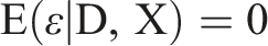
The unconfoundedness assumption or exogeneity assumption is given by

E (ε |D, X) = 0

which denotes the identification strategy. This means that we include all relevant confounders in the model and no unobserved confounders bias the results. In a naive approach to estimating the treatment effect in model (1), one might first select the relevant covariates by modern machine learning methods, such as lasso, and then estimate the treatment effect by including only the selected variables and continue with standard inference methods based on OLS. However, this procedure, while often used in applied work, might fail to provide valid post-selection inference due to the omitted variable bias. To correct for this problem, a de-biased lasso/double machine learning approach was introduced by Chernozhukov et al. (2018). To understand this approach, we introduce an auxiliary equation for the treatment variable, as follows

D = γ_{1} X_{1} + \dots + γ_{p} X_{p} + v, E (v X) = 0

(2)

For simplicity, we assume a linear relationship between D and X in this introductory example. For details on the auxiliary regression and the implementation in practice, we refer to our discussion of the model training in Nonresponse Model. The idea of double machine learning is now to run a lasso regression of the auxiliary model (2) to identify which variables create the omitted variable bias in the first step and subsequently include them in the final regression step. Hence, double machine learning can effectively be used to select all relevant variables. It can be shown that this approach leads to estimates of the target parameter that are asymptotically normally distributed (allowing valid post-selection inference). Introducing this auxiliary regression step and including omitted variables in the final regression implicitly creates a moment condition for the target parameter that fulfills the so-called Neyman orthogonality property. This means that the derivative with regard to the nuisance parameter of the corresponding score function is equal to zero at the true parameter values. Intuitively, we can see that small errors in the estimation of the nuisance parameter, as they occur under lasso, do not have a first-order effect on the treatment parameter, meaning that our estimate of the target parameter is robust to model selection mistakes. Despite selection errors in the confounders, valid results are achieved. In the naive approach, the corresponding moment condition does not fulfill this orthogonality property.

We demonstrate the different properties of the estimates received from the naive approach and the double machine learning approach by a simple simulation study of the model above with n = 100 observations and p = 100 covariates. Figure 1 shows the empirical distribution of the estimation errors ${\hat{α}}_{0} - α_{0}$ for both approaches based on 10,000 repetitions. The double machine learning estimates are nearly unbiased (centered around zero) and can be approximated by a normal distribution (see the density plot for comparison). The resulting distribution using the naive approach is highly biased (not centered around zero) and not in line with a standard normal distribution which leads to invalid post-selection inference.

Figure 1.

Distribution of 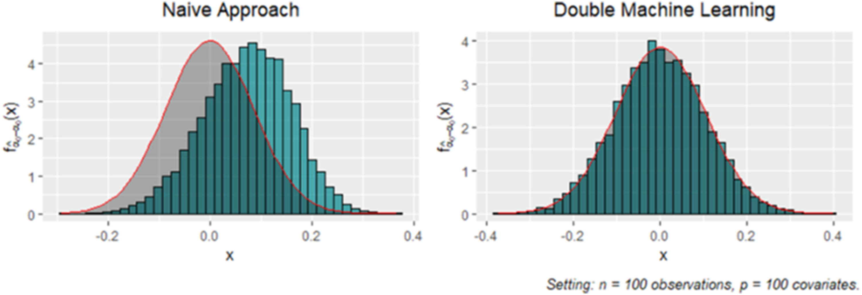${\hat{α}}_{0} - α_{0}$ for the naive approach with non-orthogonal score (left) and the double machine learning approach with orthogonal score (right).

In the following section, we show how double machine learning can be used in the context of the logistic regression model. We use this approach in our application.

Double Selection for Logistic Models

In many survey applications, the dependent outcome variable is binary, and for binary outcome variables, logistic regression is often the approach of choice. For logistic regression, the same arguments as outlined above apply when modern machine learning methods such as lasso are used to select variables and estimate the coefficients in high-dimensional linear regression models. To enable valid post-selection inference for the logistic regression, the double machine learning approach has to be modified appropriately (cf. Belloni et al., 2013).

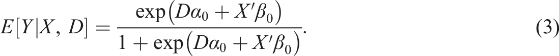
In the logistic regression, a binary dependent variable Y relates to a scalar treatment D of interest and a p-dimensional control X through a link function G

E [Y | X, D] = G (D α_{0} + X^{'} β_{0}) .

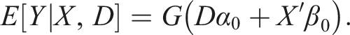
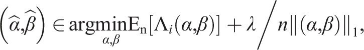
For logistic regression, the link function is given by G(t) = exp(t)/{1 + exp(t)}. We aim to perform statistical inference on the coefficient α0, which represents the impact of the treatment on the dependent variable through the link function. Estimation is usually based on the (negative) log-likelihood function associated with the logistic link function, as follows

Λ_{i} (α, β) = \log {1 + \exp (D_{i} α + {X^{'}}_{i} β)} - Y_{i} (D_{i} α + {X^{'}}_{i} β) .

For estimation in a high-dimensional setting, an ℓ1-penalty term, ${‖ (α, β) ‖}_{1} = | α | + \sum_{j = 1}^{p} | β_{j} |$ , is added to the minimization problem. The lasso logistic regression estimator is given by

(\hat{α}, \hat{β}) \in \arg \min_{α, β} E_{n} [Λ_{i} (α, β)] + λ / n {‖ (α, β) ‖}_{1},

where λ is the penalty level and

E_{n}

denotes the empirical mean. As discussed in the section above, inference on the treatment parameter α₀ is challenging and requires a modified estimation method, for example, the de-biasing lasso estimator, based on a modified moment condition. The algorithm for the de-biased estimation of the treatment parameter α₀ is presented in Algorithm 1 in Appendix B.

Application: Nonresponse Modeling for the GESIS Panel

To illustrate the double machine learning lasso, we apply the technique to model nonresponse in the 2013 recruitment to the GESIS panel.

Nonresponse in Panel Recruitment

Recruitment to a probability-based panel is arguably the most important and most expensive part of the panel life-cycle. The recruited sample needs to represent the target population and the sample size needs to be large enough to obtain precise estimates. The recruitment process usually includes several steps: contacting sampled cases and inviting them to a first recruitment survey, conducting this recruitment interview and, often during it, obtaining consent to proceed in the panel. Consenting respondents are then invited to a welcome survey (or profile survey), and those who complete it are considered to be panel members. The panel members are then surveyed on a regular basis.

Even if the regular panel waves are conducted in a self-administered mode (e.g., by mail questionnaire and/or online), it is common to approach sampled persons and conduct the recruitment interview in an interviewer-administered (face-to-face or telephone) mode (Blom et al., 2016). Respondents to the recruitment survey are then asked to proceed with the subsequent survey using cost-saving self-administered modes. This, however, includes a switch in response mode that may be subject to systematic nonresponse.

For our application, we choose nonresponse in the first interview after this switch of modes. We consider this stage to be very important for several reasons: First, this is when a large number of respondents to the recruitment survey are usually lost (for nonresponse rates in four large-scale scientific (mixed-mode) online surveys, see Blom et al. (2016)), and there is a need to understand nonresponse in order to prevent it, that is, by tackling likely nonresponse through targeted invitations (Lynn, 2020). Second, nonresponse among respondents to the face-to-face interview is costly if we consider that they have completed the cost- and labour-intensive personal interview but are no longer available to take part in the less expensive self-administered part of the panel. In addition, refreshment samples are usually planned for panels once the number of respondents has fallen below a certain minimum number. Starting with a smaller sample means that costly new recruitment is needed sooner. Third, nonresponse can introduce bias to the panel. If the respondents are not lost at random, analyses of panel data can be severely biased.

While a number of studies have been published on modeling panel attrition, for example, nonresponse to individual panel waves or dropout from the panel, the literature about correlates of nonresponse at the recruitment stages is surprisingly scarce. Comparing survey responses to official benchmarks, Sakshaug et al. (2020) analyze total recruitment error, which they define as error from initial nonresponse plus error from non-consent to be contacted again. In their comparison of a self-administered (mail/web) and CAPI recruitment, they find, for both modes, nonresponse bias to be larger than non-consent bias and total recruitment bias to be similar in both groups: both recruited samples overrepresent older and more educated population groups, currently employed persons, and higher-wage groups. They underrepresent foreign-born persons. For the GESIS recruitment panel which we also use in the present study, Bosnjak et al. (2018) compare socio-demographics of respondents of the different recruitment stages to benchmarks from the German Microcensus. They find age, citizenship, marital status, household size, place of birth, education, and household income to be distributed differently among the sample of respondents compared to the general population. The differences tend to be larger for the welcome survey than for the recruitment survey. While univariate benchmark comparisons are very useful to get an impression of bias in sample composition, they do not inform about the effect of the interplay between the respondents’ characteristics on the response decision.

Models for nonresponse in the initial recruitment survey are usually limited to only a few variables from the sample frame. The recruitment interview, however, usually generates a lot of information on the respondent that can be used to study nonresponse in the welcome survey: In addition to basic sociodemographic information, it usually also includes information on attitudes and survey experience. In interviewer-administered surveys, the interviewers often provide information about the interview situation and their expectations of the respondents’ future participation in the panel. In particular, interviewers’ ratings of a respondent’s propensity to participate in a future survey, as well as ratings of cooperativeness and enjoyment, have been found to improve nonresponse models (see, for example, Plewis et al., 2017; Sinibaldi & Eckman, 2015). Understanding the nonresponse process better can help to identify measures to address the problem, for example, through targeted invitations (Lynn, 2020).

While having a rich set of factors that potentially influence nonresponse is very helpful to understanding the nonresponse decision, it poses a challenge to nonresponse modeling. Indeed, including a large number of variables, possibly split into multiple dummy variables, and interactions requires big data solutions.

Data and Methods

The GESIS Panel Data

The GESIS panel (Bosnjak et al., 2018) is a probability-based, mixed-mode online and postal mail panel conducted bimonthly by GESIS—Leibniz Institute for the Social Sciences in Mannheim, Germany. The first cohort of the GESIS panel was recruited in 2013 and refreshment samples were recruited in 2016 and 2018. Recruitment to the GESIS panel in 2013 was based on a random sample of 21, 870 German-speaking residents of Germany aged 18 to 70 during the year of recruitment. In the first step, all sampled cases were invited to participate in a face-to-face recruitment survey. During this survey, respondents were asked for their consent to be invited to the GESIS panel by means of the online or the paper-and-pencil mode. Consenting respondents were then invited to participate in the welcome survey in the mode of their choice. Only after completing the welcome survey were respondents considered to be GESIS panel members.

In our study, we analyze nonresponse in the 2013 welcome survey among consenting respondents. We use data from the GESIS panel registration survey in 2013 (GESIS, 2020) to model nonresponse (or drop-out) (yes/no) in the subsequent welcome survey. In total, 7, 599 persons participated in the face-to-face registration survey, of whom 6, 210 agreed to being invited to the welcome survey and participating in the GESIS panel. Of these individuals, 4, 938 responded to the welcome survey and thus became regular panel members (dropout rate: 20.5%).

Nonresponse Model

For our final sample, we drop 302 observations with missing information, leaving us with 5, 908 respondents from the registration survey, of whom 4, 720 completed the welcome survey (dropout rate: 20.1%). In our analysis, we use 63 initial regressors representing information collected in the recruitment interview. This includes socio-demographic characteristics of the individuals and their cooperativeness throughout the interview. The variables we include in the analysis are listed in Table 1. We transform categorical variables into level-wise dummies and add interaction terms of the regressors. This ultimately leads to a high-dimensional logit model with a total of 329 regressors:

E [Y | X, D] = \frac{\exp (D α_{0} + X^{'} β_{0})}{1 + \exp (D α_{0} + X^{'} β_{0})} .

(3)

The binary dependent variable Y indicates nonresponse to the welcome survey. The regressors split up into 303 control variables X and 26 treatment variables D. For the treatment variables, we choose key socio-demographics, the mode the respondents chose for the welcome interview (paper-and-pencil or online questionnaire) and interviewer ratings collected in the recruitment survey. The interviewer ratings include three cooperativeness ratings and one rating of individuals’ willingness to participate in the welcome interview. The questions are:

• How would you rate the respondent’s willingness to answer the questions? (answer categories: good, moderate, low, good in the beginning but got worse, low in the beginning but got better)

• How difficult or easy was it to persuade the respondent to take part in the interview? (answer categories: very difficult, rather difficult, rather easy, very easy)

• How difficult or easy was it to persuade the respondent to take part in the follow-up interview? (answer categories: very difficult, rather difficult, rather easy, very easy)

• How likely is it that the respondent will take part in the first online- or paper questionnaire? (answer categories: very likely, rather likely, rather unlikely, very unlikely)

Table 1.

Extract of Regressors.

Treatment variables

Gender, age, nationality, education, living situation, invitation mode

Willingness to answer the questions, willingness to participate in the interview,

Willingness to participate in the panel, likelihood of participating in the welcome survey

Control variables

Migration, employment status, occupational group, life satisfaction, leisure time

Country of birth, internet use, technical affinity, survey experience,

Household size, number of children, income, incentive point

Invitation hesitance, interview intervention

Sparse categories are combined with other categories for our analysis. We recode the answer categories into good vs. bad/all other categories for “willingness to answer the questions” and combine very difficult and difficult for the two questions on the difficulty of persuading respondents to take part in the interview and follow-up interview. For the rating of the likelihood of response to the first online or paper questionnaire, we combine rather unlikely and very unlikely. With regard to sociodemographics, we include age, gender, highest educational degree, country of birth, and living situation. We generate the living situation variable from information on marital status, partnership and living in a shared household leading to the five categories: no partner; partner, not in household; partner, in household; married, living together; married, living apart. An overview of the coding for all treatment variables can be found in Table 2 in the Appendix. We include interactions of the choice of mode for the welcome survey with age, education and living situation to account for differential effects of the choice of mode on nonresponse.

Model Training

We apply the double machine learning approach introduced in Double Selection for Logistic Models for our logit model (3). The model training includes the three main steps described in Appendix B. The estimation is performed in R using the function rlassologitEffects(x,y,index), which is provided by the R-package hdm (Chernozhukov et al., 2016). The input parameter x is the matrix of our 329 regressors serving as controls and treatments. The input parameter y is our outcome variable nonresponse. The input parameter index indicates the position of variables of x which we use as treatment variables (cf. Table 1). The regression functions are estimated via post-lasso with default penalty levels

λ_{1} = 1.1 / 2 \sqrt{n} Φ^{- 1} (1 - 0.05 / \max (n, p \log (n)))

and

λ_{2} = 2.2 \sqrt{n} Φ^{- 1} (1 - 0.05 / \max (n, p \log (n)))

in Algorithm 1, where n is the number of observations (5908) and p is the total number of covariates (329) in equation (3). This choice of the penalization parameters is grounded in theory. For details, we refer to Appendix E3 in Belloni et al. (2013). In equation (2) of our general introduction to double machine learning, we consider a linear regression to model the relationship between D and the other covariates X. If we have, for example, binary treatments as in our application, a logit model might be more suitable to model the relationship between D and X. Therefore, the optimal auxiliary regression (2) strongly depends on the problem at hand. This is discussed in more detail in Appendix B.

For refined models using the double machine learning approach, we refer to the Python and R package DoubleML (Bach et al., 2021, 2022). This package provides a general implementation of the double/debiased machine learning framework and makes it possible to base inference on a large collection of classification algorithms including non-linear methods for the nuisance parameter estimation in the auxiliary regression, for example, random forests and gradient boosting. A detailed user guide for readers interested in applying the double machine learning approach can be found at https://docs.doubleml.org/stable/index.html.

Results

In this section, we present the results of our double machine learning approach to the inferential analysis of nonresponse in the GESIS panel. The results of the double lasso for logistic regression are visualized in Figures 2 –4, and a regression table can be found in Table 3 in the Appendix. We start with the interpretation of the interviewer ratings. The estimated coefficients of the interviewer ratings from the logistic regression together with the corresponding confidence intervals are displayed in Figure 2.

Figure 2.

Regression coefficients of the interviewer ratings in the logistic regression model.

Figure 3.

Regression coefficients of the socio-demographic characteristics in the logistic regression model.

Figure 4.

Regression coefficients of the chosen survey mode in the logistic regression model.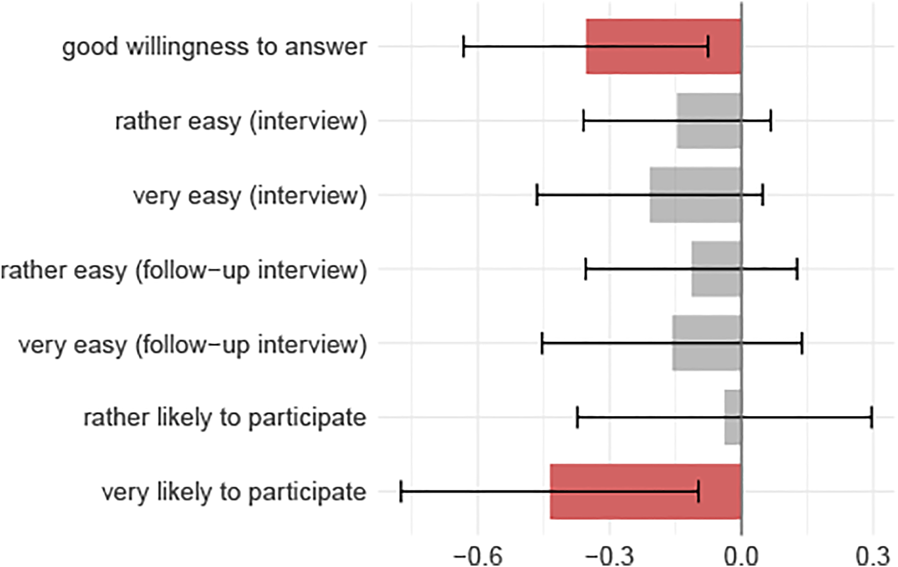

Cooperativeness

We find that the interviewer observation of respondents’ willingness to answer the survey questions in the recruitment survey had a highly significant negative effect on survey nonresponse. Respondents who were rated as having good willingness to respond to the recruitment survey dropped out of the survey after the recruitment stage to a lesser extent than respondents who were rated as having low willingness. We do not find significant effects for the ease of persuading respondents to participate in the interview nor for the ease of persuading respondents to consent to be contacted again for the follow-up interview. The effects however tend in the same direction as the observed willingness to answer the questions: respondents who were rated as being rather easy or very easy to persuade were less likely to drop-out.

Rated likelihood of participation

Respondents who were rated as being rather or very likely to participate in the welcome survey dropped out after the recruitment survey to a lesser extent than did those who were rated as being rather unlikely or very unlikely to participate. We, however, find that the only significant effect in this regard is for “very likely” category.

Socio-demographics and chosen survey mode

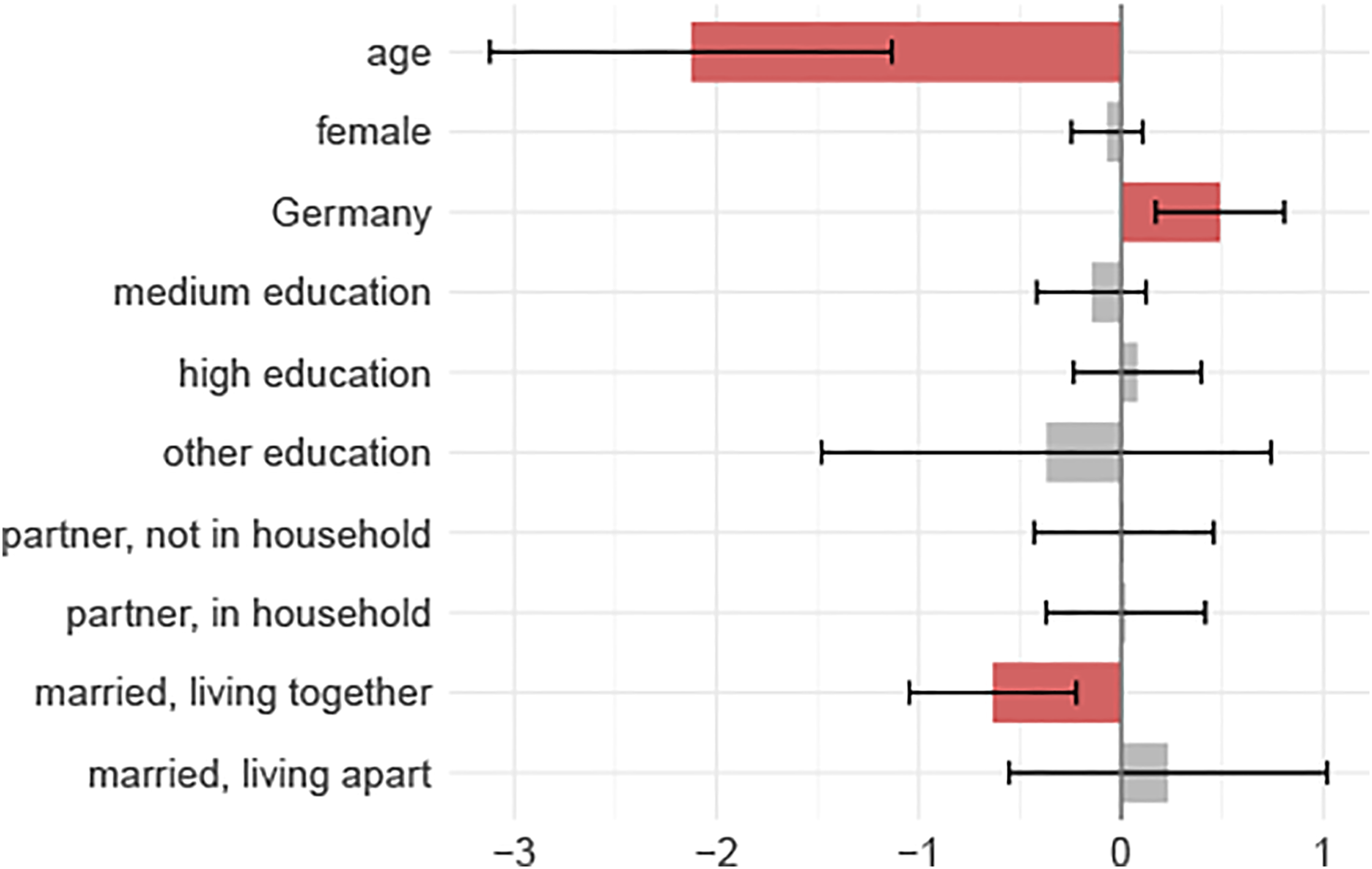
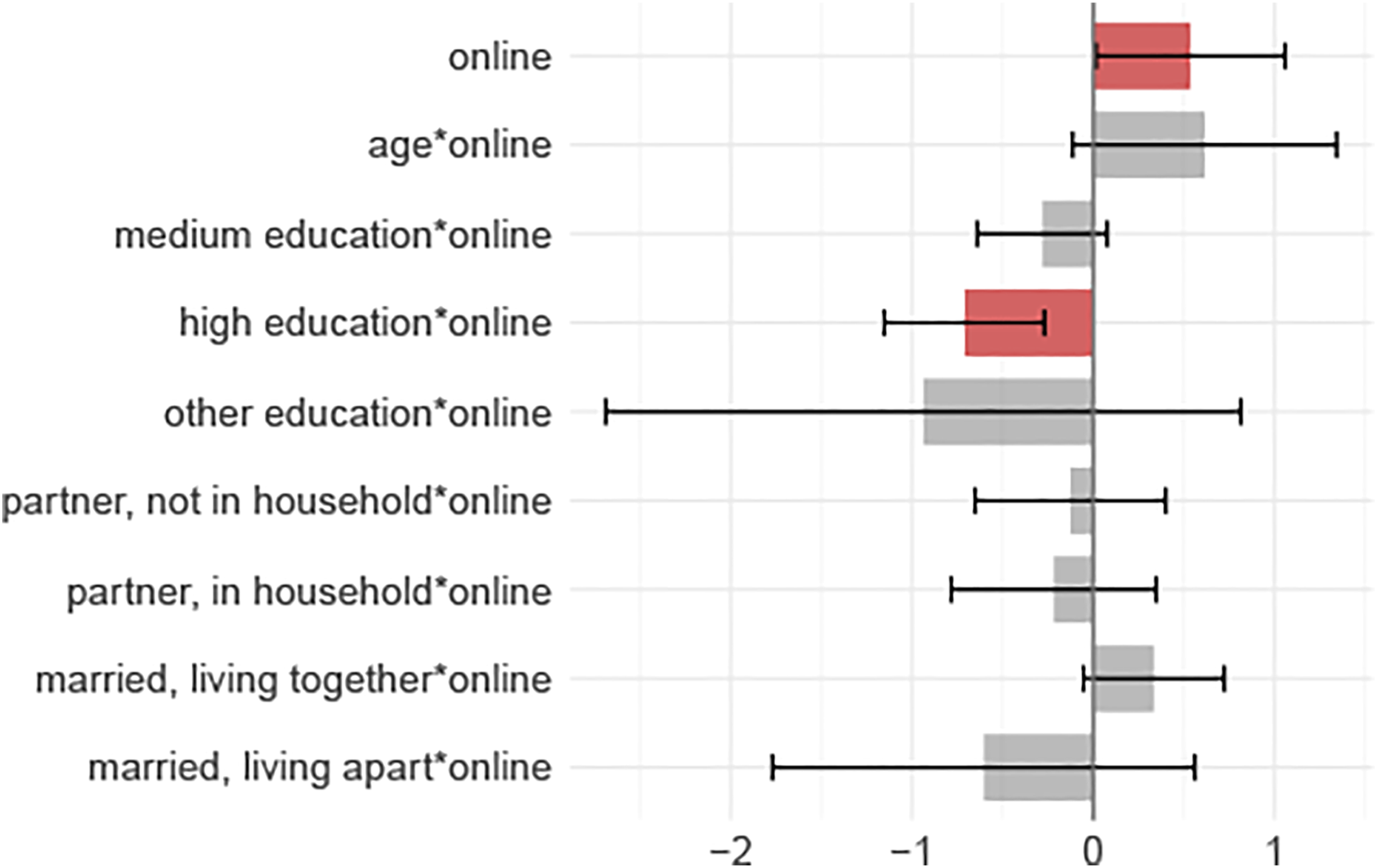
Next, we discuss the effects of socio-demographics and chosen survey mode for the welcome survey. The results are found in Figures 3 and 4.

We do not find a significant effect for respondents’ gender but do find a positive effect for having German citizenship: respondents with German citizenship dropped out after the recruitment survey at a higher rate than respondents without German citizenship.

We find that survey mode interacts with age, education (though only significantly with high education) and living situation (only being significant at the 10% level for “married, living together”). We interpret the effects of all variables that show a significant interaction with chosen survey mode. The online mode variable has a positive coefficient and is positively interacted with age, which itself has a negative coefficient. For both survey modes, we find that the older the respondents are, the lower is their likelihood to drop out after the recruitment survey. The effect is much stronger for respondents who chose the paper-and-pencil mode (−2.126) than those who chose the online mode (−1.511). Having medium, high or other education is negatively interacted with online survey mode. Medium and other education both have negative main effects and negative (though not significant) interactions with online mode. Drop-out was lower for these two groups than for respondents with low education for both survey modes and the decreasing effect is less pronounced for respondents who chose the paper-and-pencil mode than it is for those who chose the online mode. For high education, we find a positive effect on drop-out for respondents who chose the paper-and-pencil questionnaire (0.081); this turns into a negative effect for highly educated respondents who chose the online mode (−0.630). We find positive but not significant effects for the living situations “not married with partner, separate households,” “not married with partner, joint household” and “married, living apart” and negative interactions with online mode for these categories. This means that, compared to respondents who were not married and did not have a partner, the risk of drop-out was higher for respondents who chose the paper-and-pencil mode but lower for those who chose the online mode. Compared to respondents who were not married and did not have a partner, respondents who were married and lived together with their spouse showed a significant reduction in drop-out after the recruitment interview that was stronger if they chose the paper-and-pencil questionnaire (−0.634) than if they chose the online mode (−0.300).

Discussion and Conclusion

In this study, we analyze nonresponse in the welcome survey of the probability-based mixed-mode GESIS panel. Losing respondents after the face-to-face recruitment interview is not only very costly but can, through selective nonresponse, put the validity of panel inference at risk. Thus, the goal of panel recruitment should be to prevent panel drop-out among population groups that are found to be unlikely to become panel members. Knowing which population groups are likely to drop-out can help in the identification and development of targeted strategies for these groups (Lynn, 2017).

Using double machine learning for logistic regression, we are able to provide valid confidence intervals for the regression coefficients of interest and are thus able to discover significant variables that affect the likelihood to drop out. Bosnjak et al. (2018) find that the GESIS panel shows composition bias for several socio-demographic variables. We go beyond this analysis and show that these variables explain nonresponse even after controlling for several other characteristics. Furthermore, the effects of age, education, and family status are moderated by the choice of the paper-and-pencil or online survey modes. Knowing this, it might be worthwhile to develop targeted interventions that increase response depending on the mode the respondents choose. For example, older respondents who choose the paper-and-pencil mode are less likely to need an intervention than those who choose the online mode. Our findings, however, are not generalizable to countries with strongly different degrees of digitalization and different digital-divide than Germany. For the face-to-face recruited respondents of the German Internet Panel, Herzing and Blom (2019) show that age and education are associated with Internet use. If the Internet penetration within population subgroups strongly differs from Germany (e.g., only young individuals are able to respond online), the mode choices will be different than in Germany and thus our findings concerning the interactions of mode-choice and socio-demographic characteristics are not transferable.

Our study supports the findings from previous studies that interviewer ratings on the likelihood to participate in a subsequent survey are associated with respondents’ actual participation. Also, an observed good willingness to answer the questions of the survey just completed is positively associated with the likelihood to respond to a subsequent survey. While this is strong support for the usefulness of collecting such ratings in a panel survey, it is not clear, however, how to best ask interviewers to provide these. For the observed likelihood to participate in a subsequent survey, previous studies have used different scales (from 1 to 100 in Sinibaldi and Eckman (2015), from 1 to 5 in Plewis et al. (2017) and from 1 to 4 in the present study) and more research is needed on comparing these in their ability to classify respondents and explain nonresponse in a subsequent panel wave. Collecting the observed willingness to participate in follow-up surveys is only useful in a panel context. Whether collecting the observed willingness to answer the questions of the just completed questionnaire has any use beyond predicting future nonresponse, for example, in assessing response quality in a cross-sectional survey, is beyond the scope of this study.

The findings presented in this study are also limited to the nonresponse process in the face-to-face recruitment to a (mixed-mode) online panel. More research is needed on the explanation of nonresponse in different recruitment strategies. For example, recruiting respondents by mail and subsequently switching them online (see, for example, Cornesse et al., 2021) might be prone to very different nonresponse mechanisms. Furthermore, the mechanisms of nonresponse in the recruitment step are likely to differ from the mechanisms of nonresponse in subsequent waves. For example, comparing the sample composition of a panel study of employees in Germany to official benchmarks, Sakshaug and Huber (2016) find that nonresponse bias increases over time. However, the largest wave-to-wave increase in nonresponse bias occurred after the initial wave and the wave-to-wave increases get smaller over time. Future research should focus on understanding differences between nonresponse in recruitment and subsequent waves to learn more about respondents’ decision-making and find optimal ways of maintaining high motivation throughout the panel life-cycle.

The logistic regression model we consider in this paper is only one exemplary setting where double machine learning can be used for valid inference in high dimensions. The double machine learning approach can also be combined with nonlinear regression methods, like random forests, boosted trees, and neural nets, for both continuous and categorical dependent variables (Chernozhukov et al., 2018). Nevertheless, the double machine learning strategy has some limitations. First, like many statistical methods, the double machine learning strategy can only be applied to data sets that contain no missing values and cannot correct for possible measurement error in the observed variables. Second, and most crucial, it strictly relies on the unconfoundedness assumption, that is, the assumption that all relevant confounders are observed. As this assumption is not always plausible, the double machine learning approach has been adapted for the case of unobserved confounders using instrumental variables (IV) methods, see Belloni et al. (2012). In this context, Kueck et al., 2022 provide results for valid inference in an instrumental variable model when L2-Boosting is used for variable selection. Further adaptations of the double machine learning approach have been developed, for example, for causal mediation analysis (Farbmacher et al., 2022) or dynamic treatment effects estimation (Bodory et al., 2020).

The double machine learning approach can be successfully applied in all kinds of settings where researchers are interested in explaining the effects of treatment variables while controlling for a high number of covariates. Recently, many studies have been published which apply the double machine learning technique in economics, for example, to analyze gender differences in wage expectations (Bach et al., 2018a; Fernandes et al., 2021; Wunsch & Strittmatter, 2021) or to estimate the effect of policies/programs (Denisova-Schmidt et al., 2021; Goller et al., 2021; Huber et al., 2021; Knaus, 2021; Knaus et al., 2020).

In survey methodology, we intend to analyze how double machine learning might be used to select and include high numbers of control variables in imputation or weighting models. An application from political science could be the study of voting behavior on the neighborhood level, including detailed information about the socio-demographic structure, economic situation, and welfare. Another interesting research topic could be the identification of the parental effect on educational attainment during the COVID-19 pandemic, controlling for measures of children’s online behavior like social media usage. Given that social scientists are increasingly confronted with many types of big data, such as digital behavioral data and geo-spatial information of all kinds, the applications for which social scientists might benefit from the double machine learning technique are numerous.

Footnotes

Declaration of conflicting interests

The author(s) declared no potential conflicts of interest with respect to the research, authorship, and/or publication of this article.

Funding

The author(s) disclosed receipt of the following financial support for the research, authorship, and/or publication of this article: Open access was funded by the Deutsche Forschungsgemeinschaft (DFG, German Research Foundation) – Project number 491156185. Kück and Spindler acknowledge (Bach et al., 2022) financial support by the Deutsche Forschungsgemeinschaft – Project number 431701914.

ORCID iDs

Barbara Felderer

Jannis Kueck

Author Biographies

Barbara Felderer is the head of the team Survey Statistics at the Department of Survey Design and Methodology, GESIS - Leibniz-Institute for the Social Sciences. Her research focuses on survey research, especially in the area of nonresponse bias analysis and nonresponse adjustment. She recently published her research, amongst others, in the journal of official statistics and sociological methods & research.

Jannis Kueck is a postdoctoral researcher at the department of statistics at University of Hamburg. His research interests lie at the intersection of high-dimensional statistics and machine learning, in particular the combination of machine learning and causal inference. The main objective of his research is to provide new methodology for uniform inference about high-dimensional parameters in a wide range of applications. He recently published in Journal of Business and Economic Statistics, Journal of Econometrics and Biometrika.

Martin Spindler is a professor for statistics at the department of Business administration at the University of Hamburg. His research interests are machine learning and causal inference, and particularly the combination of both fields. He recently published his research, amongst others, in Biometrika, the Journal of Machine Learning Research, the Journal of Econometrics and Journal of Business and Economic Statistics.

Data and Empirical Results.

Double Machine Learning for Logistic Regression.

The double machine learning approach for logistic regression includes three main steps:

1. initial estimation of the regression function via post-lasso logistic regression,

2. estimation of instruments that are orthogonal to the weighted controls via weighted post-selection least squares, and

3. estimation of α0 based on the nuisance estimates obtained in (1) and (2).

The estimation procedure for α0 is summarized in more detail in the following algorithm:

Algorithm 1. DML for Logistic Regression

1: Run a post-lasso-logistic regression of Yi on Di and Xi

\begin{array}{l} (\hat{α}, \hat{β}) \in \arg \min_{α, β} E [Λ_{i} (α, β)] + λ_{1} / n {‖ (α, β) ‖}_{1}, \\ (\tilde{α}, \tilde{β}) \in \arg \min_{α, β} E [Λ_{i} (α, β)] : support (β) \subset support (\tilde{β}), \end{array}

where Λi (α, β) is the (negative) log-likelihood function associated with the logistic link function. For i = 1, …, n, keep the value

${X^{'}}_{i} \tilde{β}$ and the weight

${\hat{ω}}_{i}$ which is defined as

{\hat{ω}}_{i} = {\hat{σ}}_{i}^{2} = V a r (Y_{i} | D_{i}, X_{i}) = G (D_{i} \tilde{α} + {X^{'}}_{i} \tilde{β}) {1 - G (D_{i} \tilde{α} + {X^{'}}_{i} \tilde{β})}

with the logistic link function G(t) = exp(t)/{1 + exp(t)}

2: Run a post-lasso OLS regression of $\sqrt{{\hat{ω}}_{i}} D_{i}$ on $\sqrt{{\hat{ω}}_{i}} X_{i}$ :

$\begin{array}{l} \hat{θ} \in \arg \min_{θ} E [{\hat{ω}}_{i} {(D_{i} - {X^{'}}_{i} θ)}^{2}] + λ_{2} / n {‖ Γ θ ‖}_{1}, \\ \tilde{θ} \in \arg \min_{θ} E [{\hat{ω}}_{i} {(D_{i} - {X^{'}}_{i} θ)}^{2}] : support (θ) \subset support (\hat{θ}) . \end{array}$

Keep the residual ${\hat{v}}_{i} : = \sqrt{{\hat{ω}}_{i}} (D_{i} - {X^{'}}_{i} \tilde{θ})$ and instrument

{\hat{z}}_{i} : = {\hat{v}}_{i} / \sqrt{{\hat{ω}}_{i}}, i = 1, \dots, n

3: Run an instrumental logistic regression of $Y_{i} - {X^{'}}_{i} \tilde{β}$ on Di using

${\hat{z}}_{i}$ as the instrument for Di

\overset{\lor}{α} \in \arg \inf_{α \in A} L_{n} (α),

where

L_{n} (α) = \frac{{| E_{n} [{Y_{i} - G (D_{i} α + {X^{'}}_{i} \tilde{β})} {\hat{z}}_{i}] |}^{2}}{E_{n} [{Y_{i} - G (D_{i} α + {X^{'}}_{i} \tilde{β})}^{2} {\hat{z}}_{i}^{2}]}

and $A = {α \in ℝ : | α - \tilde{α} | \leq C / \log n}$ . Compute the confidence region with asymptotic coverage 1 − ξ:

{α \in ℝ : | α - \tilde{α} | \leq {\hat{Σ}}_{n} Φ^{- 1} (1 - ξ / 2) / \sqrt{n}}

For the estimator of the variance

{\hat{Σ}}_{n}

and details about the Algorithm 1, we refer to Belloni et al. (2016). Applying the double machine learning approach, Belloni et al. (2016) consider the following auxiliary regression

\sqrt{ω_{i}} D_{i} = \sqrt{ω_{i}} {X^{'}}_{i} θ_{0} + v_{i}, E [\sqrt{ω_{i}} v_{i} X_{i}] = 0

where the weight ωi is defined as the conditional variance of the outcome Yi given Di and Xi. Using this auxiliary regression, they construct the instruments

z_{i} = D_{i} - {X^{'}}_{i} θ_{0}

(cf. step 2 of Algorithm 1) that are necessary for valid inference in high dimensions. It is worth noting that the projection

{X^{'}}_{i} θ_{0}

is only defined as the best linear approximation of Di and there is no distributional assumption on ν, except conditions on the moments (cf. Condition L in Belloni et al. (2016)). Nevertheless, we could also construct instruments using the conditional expectation of Di given Xi, m0(Xi) = E[Di|Xi]. If we want to model the conditional expectation, we need to adjust the auxiliary regression in step 2 in Algorithm 1 for each treatment Di depending on the type of the treatment (binary, nominal, continuous). Note that even if we consider the following regression model

\sqrt{ω_{i}} D_{i} = \sqrt{ω_{i}} m_{0} (X_{i}) + {\tilde{v}}_{i}, E [\sqrt{ω_{i}} {\tilde{v}}_{i} | X_{i}] = 0

for a continuous treatment Di, the function m0 could satisfy different structured properties depending on the problem at hand. Such properties motivate the use of different estimators for m0 in high dimensions. If one assumes a sparse linear model, as we did in Algorithm 1, it permits the use of lasso or post-lasso to estimate θ0. On the other hand, we can use ridge estimators if we assume that

m_{0} (X_{i}) = {X^{'}}_{i} θ_{0}

is dense with respect to X. If we do not want to assume linearity, we could also use non-linear estimation methods like random forests or boosted trees for the estimation of the auxiliary regression.

References

Bach

Chernozhukov

Kurz

M. S.

Spindler

(2021). DoubleML – An object-oriented implementation of double machine learning in R. arXiv: 2103.09603 [stat.ML].

Bach

Chernozhukov

Kurz

M. S.

Spindler

(2022). Doubleml – an object-oriented implementation of double machine learning in python. Journal of Machine Learning Research, 23(53), 1–6.

Bach

Chernozhukov

Spindler

(2018a). Closing the us gender wage gap requires understanding its heterogeneity. arXiv preprint arXiv: 1812.04345.

Bach

Chernozhukov

Spindler

(2018b). Valid simultaneous inference in high-dimensional settings (with the hdm package for R). Papers 1809.04951, arXiv.org.

Belloni

Chen

Chernozhukov

Hansen

(2012). Sparse models and methods for optimal instruments with an application to eminent domain. Econometrica, 80(6), 2369–2429.

Belloni

Chernozhukov

Fernández-Val

Hansen

(2017). Program evaluation and causal inference with high-dimensional data. Econometrica, 85(1), 233–298. https://doi.org/10.3982/ecta12723

Belloni

Chernozhukov

Hansen

(2014a). High-dimensional methods and inference on structural and treatment effects. Journal of Economic Perspectives, 28(2), 29–50. https://doi.org/10.1257/jep.28.2.29

Belloni

Chernozhukov

Hansen

(2014b). Inference on treatment effects after selection amongst high-dimensional controls. Review of Economic Studies, 81(2), 608–650. https://doi.org/10.1093/restud/rdt044

Belloni

Chernozhukov

Wei

(2013). Honest confidence regions for a regression parameter in logistic regression with a large number of controls. Cemmap Working Paper CWP67/13

10.

Belloni

Chernozhukov

Wei

(2016). Post-selection inference for generalized linear models with many controls. Journal of Business & Economic Statistics, 34(4), 606–619. https://doi.org/10.1080/07350015.2016.1166116

11.

Blom

A. G.

Bosnjak

Cornilleau

Cousteaux

A.-S.

Das

Douhou

Krieger

(2016). A comparison of four probability-based online and mixed-mode panels in Europe. Social Science Computer Review, 34(1), 8–25. https://doi.org/10.1177/0894439315574825

12.

Bodory

Huber

Lafférs

(2020). Evaluating (weighted) dynamic treatment effects by double machine learning. arXiv preprint arXiv:2012.00370.

13.

Bosnjak

Dannwolf

Enderle

Schaurer

Struminskaya

Tanner

Weyandt

K. W.

(2018). Establishing an open probability-based mixed-mode panel of the general population in Germany: The gesis panel. Social Science Computer Review, 36(1), 103–115. https://doi.org/10.1177/0894439317697949

14.

Breiman

(2001). Statistical modeling: The two cultures (with comments and a rejoinder by the author). Statistical Science, 16(3), 199–231. https://doi.org/10.1214/ss/1009213726

15.

Buskirk

T. D.

(2018). Surveying the forests and sampling the trees: An overview of classification and regression trees and random forests with applications in survey research. Survey Practice, 11(1), 1–13. https://doi.org/10.29115/sp-2018-0003

16.

Buskirk

T. D.

Kirchner

Eck

Signorino

C. S.

(2018). An introduction to machine learning methods for survey researchers. Survey Practice, 11(1), 1–10. https://doi.org/10.29115/sp-2018-0004

17.

Buskirk

T. D.

Kolenikov

(2015). Finding respondents in the forest: A comparison of logistic regression and random forest models for response propensity weighting and stratification. Survey Insights: Methods from the Field. https://surveyinsights.org/?p=5108

18.

Callegaro

(2013). Paradata in web surveys. In Kreuter

(Ed.), Improving surveys with paradata: Analytic uses of process information (pp. 261–279). John Wiley & Sons

19.

Chernozhukov

Chetverikov

Demirer

Duflo

Hansen

Newey

Robins

(2018). Double/debiased machine learning for treatment and structural parameters. The Econometrics Journal, 21(1), C1–C68. https://doi.org/10.1111/ectj.12097

20.

Chernozhukov

Hansen

Spindler

(2015). Valid post-selection and post-regularization inference: An elementary, general approach. Annual Review of Economics, 7(1), 649–688. https://doi.org/10.1146/annurev-economics-012315-015826

21.

Chernozhukov

Hansen

Spindler

(2016). Hdm: High-dimensional metrics. The R Journal, 8(2), 185–199. https://doi.org/10.1920/wp.cem.2016.3716

22.

Cornesse

Felderer

Fikel

Krieger

Blom

A. G.

(2021). Recruiting a probability-based online panel via postal mail: Experimental evidence. Social Science Computer Review. https://doi.org/10.1177/08944393211006059.

23.

Denisova-Schmidt

Huber

Leontyeva

Solovyeva

(2021). Combining experimental evidence with machine learning to assess anti-corruption educational campaigns among russian university students. Empirical Economics, 60(4), 1661–1684. https://doi.org/10.1007/s00181-020-01827-1

24.

Durrant

G. B.

Steele

(2009). Multilevel modelling of refusal and non-contact in household surveys: Evidence from six uk government surveys. Journal of the Royal Statistical Society: Series A (Statistics in Society), 172(2), 361–381. https://doi.org/10.1111/j.1467-985x.2008.00565.x

25.

Earp

Mitchell

McCarthy

Kreuter

(2014). Modeling nonresponse in establishment surveys: Using an ensemble tree model to create nonresponse propensity scores and detect potential bias in an agricultural survey. Journal of Official Statistics, 30(4), 701–719. https://doi.org/10.2478/jos-2014-0044

26.

Eck

(2018). Neural networks for survey researchers. Survey Practice, 11(1), 1–11. https://doi.org/10.29115/SP-2018-0002

27.

Farbmacher

Huber

Lafférs

Langen

Spindler

(2022). Causal mediation analysis with double machine learning. The Econometrics Journal. https://doi.org/10.1093/ectj/utac003.

28.

Feddersen

Metcalfe

Wooden

(2016). Subjective wellbeing: Why weather matters. Journal of the Royal Statistical Society: Series A (Statistics in Society), 179(1), 203–228. https://doi.org/10.1111/rssa.12118

29.

Fernandes

Huber

Vaccaro

(2021). Gender differences in wage expectations. Plos One, 16(6), e0250892. https://doi.org/10.1371/journal.pone.0250892

30.

GESIS (2020). Gesis panel - standard edition. GESIS Datenarchiv. Köln. ZA5665 Datenfile Version 37.0.0 https://doi.org/10.4232/1.13573

31.

Goller

Harrer

Lechner

Wolff

(2021).Active labour market policies for the long-term unemployed: New evidence from causal machine learning. arXiv preprint arXiv:2106.10141.

32.

Herzing

J. M. E.

Blom

A. G.

(2019). The influence of a person’s digital affinity on unit nonresponse and attrition in an online panel. Social Science Computer Review, 37(3), 404–424. https://doi.org/10.1177/0894439318774758

33.

Huber

Meier

Wallimann

(2021). Business analytics meets artificial intelligence: Assessing the demand effects of discounts on swiss train tickets. arXiv preprint arXiv:2105.01426

34.

Imbens

G. W.

Rubin

D. B.

(2015). Causal inference for statistics, social, and Biomedical sciences: An introduction. Cambridge University Press

35.

Japec

Kreuter

Berg

Biemer

Decker

Lampe

Lane

O’Neil

Usher

(2015). Big data in survey research: AAPOR task force report. Public Opinion Quarterly, 79(4), 839–880. https://doi.org/10.1093/poq/nfv039

36.

Kern

Klausch

Kreuter

(2019a). Tree-based machine learning methods for survey research. Survey Research Methods, 13(1), 73–93. https://doi.org/10.18148/srm/2019.v1i1.7395

37.

Kern

Weiss

Kolb

J.-P.

(2021). Predicting nonresponse in future waves of a probability-based mixed-mode panel with machine learning. Journal of Survey Statistics and Methodology. https://doi.org/10.1093/jssam/smab009.

38.

Kirchner

Signorino

C. S.

(2018). Using support vector machines for survey research. Survey Practice, 11(1), 1–14. https://doi.org/10.29115/sp-2018-0001

39.

Knaus

M. C.

(2021). A double machine learning approach to estimate the effects of musical practice on student’s skills. Journal of the Royal Statistical Society: Series A (Statistics in Society), 184(1), 282–300. https://doi.org/10.1111/rssa.12623

40.

Knaus

M. C.

Lechner

Strittmatter

(2020). Heterogeneous employment effects of job search programmes: A machine learning approach. Journal of Human Resources, 57(2), 597-636.

41.

Kreuter

(2013a). Facing the nonresponse challenge. The ANNALS of the American Academy of Political and Social Science, 645(1), 23–35. https://doi.org/10.1177/0002716212456815

42.

Kreuter

(2013b). Improving surveys with paradata: Analytic uses of process information. John Wiley & Sons

43.

Kueck

Luo

Spindler

Wang

(2022). Estimation and inference of treatment effects with L₂-boosting in high-dimensional settings. Journal of Econometrics. https://doi.org/10.1016/j.jeconom.2022.02.005.

44.

Liu

(2020). Using machine learning models to predict attrition in a survey panel. In Hill

C. A.

Biemer

P. P.

Buskirk

T. D.

Japec

Kirchner

Kolenikov

Lyberg

L. E.

(Eds.), Big data meets survey science: A collection of innovative methods (pp. 415–433). John Wiley & Sons.

45.

Lynn

(2017). From standardised to targeted survey procedures for tackling non-response and attrition. Survey Research Methods, 11(1), 93-103. https://doi.org/10.18148/srm/2017.v11i1.6734.

46.

Lynn

(2020). Methods for recruitment and retention. Understanding Society Working Paper 2020-07. Understanding Society at the

Institute for Social and Economic Research

47.

Murphy

Link

M. W.

Childs

J. H.

Tesfaye

C. L.

Dean

Stern

Pasek

Cohen

Callegaro

Harwood

(2014). Social media in public opinion research: Executive summary of the aapor task force on emerging technologies in public opinion research. Public Opinion Quarterly, 78(4), 788–794. https://doi.org/10.1093/poq/nfu053

48.

Phipps

Toth

(2012). Analyzing establishment nonresponse using an interpretable regression tree model with linked administrative data. The Annals of Applied Statistics, 6(2), 772–794. https://doi.org/10.1214/11-aoas521

49.

Plewis

Calderwood

Mostafa

(2017). Can interviewer observations of the interview predict future response? Methods, Data, Analyses, 11(1), 1-16. https://doi.org/10.12758/mda.2016.010.

50.

Roßmann

Gummer

(2016). Using paradata to predict and correct for panel attrition. Social Science Computer Review, 34(3), 312–332. https://doi.org/10.1177/0894439315587258

51.

Sakshaug

J. W.

Huber

(2016). An evaluation of panel nonresponse and linkage consent bias in a survey of employees in germany. Journal of Survey Statistics and Methodology, 4(1), 71–93. https://doi.org/10.1093/jssam/smv034

52.

Sakshaug

J. W.

Hülle

Schmucker

Liebig

(2020). Panel survey recruitment with or without interviewers? Implications for nonresponse, panel consent, and total recruitment bias. Journal of Survey Statistics and Methodology, 8(3), 540–565. https://doi.org/10.1093/jssam/smz012

53.

Shmueli

(2010). To explain or to predict? Statistical Science, 25(3), 289–310. https://doi.org/10.1214/10-sts330

54.

Signorino

C. S.

Kirchner

(2018). Using lasso to model interactions and nonlinearities in survey data. Survey Practice, 11(1), 1–10. https://doi.org/10.29115/sp-2018-0005

55.

Sinibaldi

Eckman

(2015). Using call-level interviewer observations to improve response propensity models. Public Opinion Quarterly, 79(4), 976–993. https://doi.org/10.1093/poq/nfv035

56.

Struminskaya

Lugtig

Keusch

Höhne

J. K.

(2020). Augmenting surveys with data from sensors and apps: Opportunities and challenges. Social Science Computer Review. https://doi.org/10.1177/0894439320979951.

57.

Wunsch

Strittmatter

(2021). The gender pay gap revisited with big data: Do methodological choices matter? CESifo Working Paper No. 8912

58.

Zinn

Gnambs

(2020). Analyzing nonresponse in longitudinal surveys using bayesian additive regression trees: A nonparametric event history analysis. Social Science Computer Review. https://doi.org/10.1177/0894439320928242.

Using Double Machine Learning to Understand Nonresponse in the Recruitment of a Mixed-Mode Online Panel

Abstract

Keywords

Introduction

(Double) Machine Learning

Basic Setting and Idea behind Double Machine Learning

Double Selection for Logistic Models

Application: Nonresponse Modeling for the GESIS Panel

Nonresponse in Panel Recruitment

Data and Methods

The GESIS Panel Data

Nonresponse Model

Model Training

Results

Cooperativeness

Rated likelihood of participation

Socio-demographics and chosen survey mode

Discussion and Conclusion

Footnotes

Declaration of conflicting interests

Funding

ORCID iDs

Author Biographies

Data and Empirical Results.

Double Machine Learning for Logistic Regression.

References