Sage Journals: Discover world-class research

Abstract

Increasing nonresponse rates is a pressing issue for many longitudinal panel studies. Respondents frequently either refuse participation in single survey waves (temporary dropout) or discontinue participation altogether (permanent dropout). Contemporary statistical methods that are used to elucidate predictors of survey nonresponse are typically limited to small variable sets and ignore complex interaction patterns. The innovative approach of Bayesian additive regression trees (BART) is an elegant way to overcome these limitations because it does not specify a parametric form for the relationship between the outcome and its predictors. We present a BART event history analysis that allows identifying predictors for different types of nonresponse to anticipate response rates for upcoming survey waves. We apply our novel method to data from the German National Educational Panel Study including N = 4,559 students in Grade 5 that observed nonresponse rates of up to 36% across five waves. A cross-validation and comparison with logistic regression models with least absolute shrinkage and selection operator penalization underline the advantages of the approach. Our results highlight the potential of Bayesian discrete-time event modeling for the long-term projection of panel stability across multiple survey waves. Finally, potential applications of this approach for operational use in survey management are outlined.

Keywords

panel study dropout nonresponse regression tree Bayes

Unit nonresponse presents an increasing obstacle for longitudinal social surveys and educational large-scale assessments, which threatens the representativeness of samples and compromises the validity of conclusions drawn from these data (Beullens et al., 2018; Kreuter, 2013; Williams & Brick, 2017). Specifically, biased population estimates might result from incomplete data if observed responses differ systematically from responses that could have been theoretically obtained from nonresponding units (e.g., Heffetz & Reeves, 2019; Trappmann et al., 2015). Therefore, longitudinal panel studies strive to prevent nonresponse from the outset and delay panel mortality (i.e., withdrawal of participants) as long as possible. For this purpose, it is important to identify already at an early stage participants with a high nonresponse propensity in order to implement appropriate intervention strategies (e.g., providing more attractive incentives; see Felderer et al., 2018; McGovern et al., 2018). The primary objective of this article is the introduction of a novel approach for the prediction of future participation behavior in longitudinal surveys that allow implementing countermeasures to prevent nonresponse. So far, most nonresponse research takes a rather short-term perspective and focuses on wave-to-wave participation rates, that is, the share of nonresponders in a given wave as compared to the sample in the previous wave (e.g., Durrant & Steele, 2009; Roßmann & Gummer, 2016; West, 2013). As a consequence, most findings are rather limited in scope and do not allow for long-term projections of panel stability. Moreover, statistical methods commonly used for the analysis of nonresponse (e.g., logistic regression) are ill-equipped to handle large and complex predictor sets (see, e.g., van Smeden et al., 2019) that are typically available in longitudinal panel studies. In practice, survey researchers frequently limit their analyses to variable main effects (or, at the most, bivariate interactions) while ignoring higher order interaction and nonlinear effect patterns thus sacrificing a potential gain in precision for statistical efficiency. Therefore, this study proposes a tree-based method that is suitable for handling complex variable sets for analyzing panel attrition (Chipman et al., 2010) and using nonparametric event history analyses to examine nonresponse across multiple survey waves. Because the relationship between predictors and outcome does not assume a parametric form (as is the case with, e.g., linear regression), the adopted machine learning approach places few restrictions on potential effect patterns (e.g., nonlinearity, interactions). As a result, it allows for more valid inferences on important predictors of participation propensities in social surveys. We applied our method to data from the longitudinal German National Educational Study (Blossfeld et al., 2011) to predict participation rates across five survey waves and identify relevant predictors for different types of nonresponse.

The Problem of Nonresponse in Longitudinal Surveys

Panel studies require repeated participation of sampling units across long periods of time. However, many respondents are reluctant to invest the sustained effort required for this task and refuse follow-up invitations to surveys (e.g., Kleinert et al., 2019; Williams & Brick, 2017). Unit nonresponse resulting from a refusal to participate in a study is commonly referred to as dropout, break off, or attrition (Brüderl & Trappmann, 2017; Peytchev, 2009) and represents an increasing problem in social science research. For example, Zinn and Gnambs (2018) observed a dropout rate in a longitudinal German large-scale assessment across 4 years of up to 61%. Continually decreasing response rates in social surveys seem to be a global trend. For recent rounds of the European Social Survey, the decline in response rates across 36 countries was around 1–1.5 percentage points from one wave to another, resulting in overall response rates as low as 35% for some countries despite extensive fieldwork efforts (Beullens et al., 2018). More importantly, sampling units declining survey participation frequently exhibit systematically different characteristics than participants (e.g., Heffetz & Reeves, 2019; Trappmann et al., 2015; Voorpostel & Lipps, 2011). For example, specific life events such as changes in employment status or household composition tend to increase nonresponse in longitudinal social surveys (Trappmann et al., 2015); in contrast, continuous respondents across multiple survey waves tend to report fewer life changes (Voorpostel & Lipps, 2011). Thus, nonresponse can seriously undermine the validity of representative social surveys.

Generally, unit nonresponse refers to the loss of sampling units drawn from the population. In longitudinal studies, unit nonresponse can be further distinguished into two types (Müller & Castiglioni, 2020): respondents refusing participation in a given wave but participating in upcoming waves of the panel study (temporary dropout) and respondents refusing participation in a given wave and any upcoming waves (permanent dropout). Recent studies showed that temporary dropout cases systematically differ from continuous respondents and more strongly resemble permanent dropout cases (Michaud et al., 2011; Watson & Wooden, 2014). Therefore, preventing nonresponds in the first place seems to be a way of improving sample variability and mitigating the biasing effect of permanent dropout in panel studies (Müller & Castiglioni, 2020). This requires identifying candidate nonresponders that might be persuaded to reengage with a panel study in the future and developing respective incentive strategies for hard-to-survey respondents (cf. Adhikari & Bryant, 2018). Ideally, the dropout propensity of sampling units in a panel study is even identified before unit nonresponse actually occurred. Then, respective counterstrategies can be devised that prevent dropout (see Earp et al., 2014). Moreover, identifying participation trajectories already early on in a panel study can help planning timelines for sample refreshments and evaluating budgetary requirements. However, this requires accurate prediction models that can estimate the likelihood of temporary and permanent dropout across multiple waves of a longitudinal study.

Regression Trees for Analyzing Survey Participation

Regression relationships in survey data are often complex including many covariates, nonlinear effects, and higher order interactions. Machine learning methodologies offer flexible modeling techniques that can accommodate these complex data structures and allow studying survey participation without requiring the a priori specification of a functional form between nonresponse and its predictors. Contemporary machine learning methods (see Kuhn & Johnson, 2013, for an overview) are also particularly well-equipped to handle large predictor sets that are typically available in social surveys (e.g., respondent characteristics, survey responses, paradata). Thus, recent reviews highlighted the potential of machine learning techniques also for survey research (e.g., Buskirk et al., 2018; Kern et al., 2019; Toth & Phipps, 2014), for example, for adaptive data collection (e.g., identifying additional cases during field time), nonresponse adjustments (e.g., correcting for unequal participation probabilities), and nonresponse analyses (e.g., describing dropout patterns). Particularly, tree-based methods have been shown to outperform commonly used prediction techniques such as logistic regression (Buskirk & Kolenikov, 2015; Phipps & Toth, 2012). Therefore, the next sections introduce the idea of classification and regression trees (CART; Breiman et al., 1984) and their extension to Bayesian additive regression trees (BART; Chipman et al., 2010). Finally, we show how BART can be used to examine different types of nonresponse using event history modeling.

The Basics of Regression Trees

Tree-based methods such as CART (Breiman et al., 1984) employ a recursive partitioning algorithm to build a tree structure by splitting a sample into mutually exclusive classes (so-called terminal nodes) according to the predictor space (see Figure 1). Let the random variable Y with the realization y_i for respondent $i \in \{1, ..., I\}$ represents a binary outcome indicating survey (non)participation and x_i a Q dimensional vector of predictors. Starting with the entire sample, the algorithm minimizes the loss function used for model evaluation (e.g., the entropy or the mean squared error) and searches for a decision rule that results in the best split leading to the two most homogenous classes with respect to Y. The decision rule is a binary split of a single predictor s of all available predictors X, $s \in X$ , and a cut point c such that {s < c} versus {s ≥ c} for a continuous s or {s = c} versus {s ≠ c} for a categorical s. After the decision rule is found, the resulting classes are themselves considered for splitting. This process is repeated until a prespecified termination criterion (e.g., minimum number of cases per node) is reached. Finally, the tree consists of B terminal nodes and associated parameter values $M \in \{μ_{1}, ..., μ_{B}\}$ that can be used for predicting the outcome for new data. M represents the E(Y|x) in each terminal node, that is, the modal category of Y. Thus, given a tree structure T with its nodes and decision rules and the parameter values M for each terminal node, the regression relationship between y_i and x_i can be formally expressed as

Figure 1.

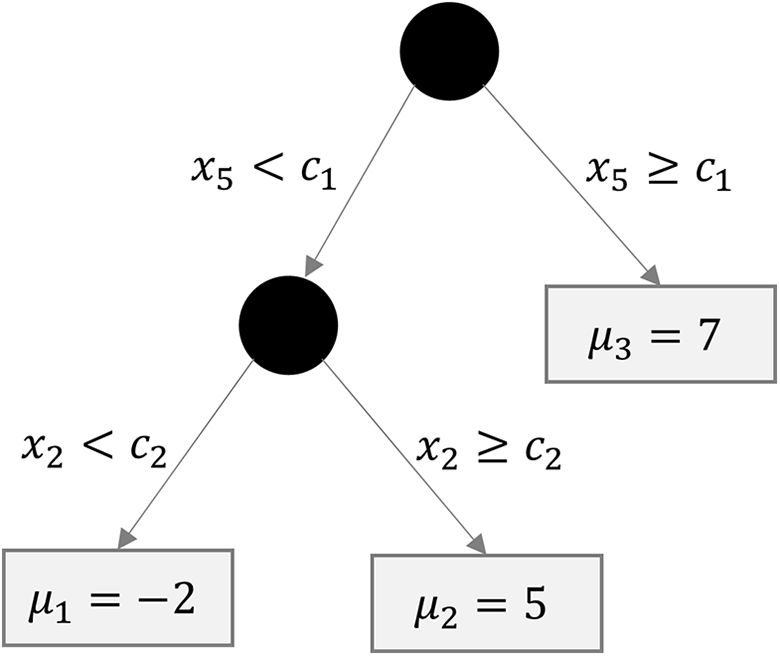
Example of a regression tree of depth d = 2 with two splits (including cut scores c₁ and c₂) and m = 3 terminal nodes.

y_{i} = g (x_{i}; T, M) + ε_{i},

where $ε_{i} \sim N (0, σ^{2})$ with g as a function describing the tree. Because g(x_i; T, M) in Equation (1) returns the $μ_{b} \in M$ assigned to x_i, E(Y|x_i) corresponds to the terminal node parameter μ _b given by g(x_i; T, M).

In contrast to single tree–based methods, ensemble methods combine multiple trees and, thus, tend to achieve better predictive performance. A particularly versatile development in this area is BART (Chipman et al., 2010).

Bayesian Additive Regression Trees

The BART model is a sum-of-trees approach with regularization priors on the model parameters. In contrast to CART models, multiple trees are combined in an additive fashion as

y_{i} = \sum_{l = 1}^{m} g (x_{i}; T_{l}, M_{l}) + ε_{i},

where $ε_{i} \sim N (0, σ^{2}) .$ Under Equation (2), E(Y|x_i) is the sum of all parameter values μ _bl for the terminal nodes assigned to x_i by g(x_i; T_l, M_l). Although the number of trees m can be specified as an unknown parameter in the Bayesian implementation of Equation (2), the computational costs are high and do not seem to offer a substantial gain in prediction accuracy as compared to selecting a default value of 200 (Chipman et al., 2010). Typically, the predictive performance of BART strongly increases among smaller numbers of trees and then levels off.

Assuming prior independence, the model uses priors for three components: a prior p(T_l) for the tree structure, a prior p(μ _bl |T_l) for the parameter values in the terminal nodes given the tree structure, and a prior p(σ) for the variance. The regularization prior p(T_l) determines the depth $d \in [1, \infty)$ of tree l and assigns prior probabilities of $α {(1 + d)}^{- β}$ with $α \in (0, 1)$ and $β \in [0, \infty)$ to each node that it is a nonterminal node and can be used for another split. Chipman and colleagues (2010) recommend using α = .95 and β = 2 as default values, which give the largest probabilities to smaller trees of depth d = 2 or 3 (although larger trees with many terminal nodes can also emerge given the data). The prior p(μ _bl |T_l) for the terminal node values is

μ_{b l} \sim N (0, σ_{μ}^{2}),

where $σ_{μ} = e / (k \sqrt{m})$ which assigns lower probabilities to extreme values and effectively shrinks the μ _bl toward zero. In doing so, each individual tree in Equation (2) explains only a small portion of the outcome and can also be interpreted as a “weak learner.” For binary outcomes, the recommended choice for e is 3.0, whereas a value of 2 has been suggested for k, which yields a 95% prior probability that E(Y|x) falls between the observed minimum and maximum values of an appropriately rescaled Y (Chipman et al., 2010). Finally, an inverse χ² distribution can be used as a prior for the variance σ² (see again Chipman et al., 2010). However, as our discrete-time event models (see below) use a probit regression with latent variables and unit variance (σ² = 1) for our purposes, no further prior specification is required.

The BART model is estimated using a Gibbs sampler with a Bayesian backfitting Markov Chain Monte Carlo (MCMC) algorithm embedded (Hastie & Tibshirani, 2000). That is, upon each sequence of draws from the full conditional distributions of the unknown parameters T_l, M_l, and σ, the partial residuals are derived as

R_{l} \equiv y - \sum_{k \neq l} g (x; T_{k}, M_{k})

on a fit that excludes the lth tree. In each step of the Gibbs sampler (referring to the conditional density of the parameters T_l and M_l of the tree l), these are then used as the conditional variables instead of all the trees T_k and parameter sets M_k that exclude T_l and M_l. The conditional tree structure (T_l|R_l, σ) is drawn using a Metropolis–Hastings step (Chipman et al., 1998), whereas the conditional terminal node values (M_l|T_l, R_l, σ) are drawn from a normal distribution. Finally, conditional on all T_l and M_l, the residual SD (σ|T₁,…, T_m, M₁,…, M_m) is drawn from an inverse gamma distribution. In our case, the last step is dropped since we use a probit specification to fit discrete-time event history models (see below). This backfitting algorithm generates a sequence of draws of (T₁, M₁)…(T_m, M_m) that converge to the posterior distribution of the true model

p (\sum_{l = 1}^{m} g (\cdot; T_{l}, M_{l}) | Y) .

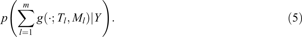
The posterior distribution can be used to calculate Bayesian inferential statistics such as posterior means or medians and respective credibility intervals. Further information on the estimation algorithm is given in the study of Chipman et al. (2010) and Kapelner and Bleich (2016).

The predictor importance in tree-based methods is evaluated by focusing on the subset of variables that was used for splitting and growing the trees. Various backward stepwise selection procedures have been suggested that quantify, for example, the reduction in mean square error (Díaz-Uriarte & de Andrés, 2006) or posterior predictive uncertainty within nodes (Gramacy et al., 2013) to rank predictors by importance. In BART, Chipman and colleagues (2010) suggested the variable inclusion proportion p_vi, that is, the posterior mean of the relative number of times a given variable is used in a tree decision rule. Because predictors with large p_vi are likely to be important drivers of the outcome, p_vi can be used to rank the predictors in x in terms of importance. Note that the p_vi are indicators of relative importance and do not reflect whether any given covariate has a “real effect” (Bleich et al., 2014). In situations where all variables are unrelated to Y, BART would select covariates randomly to grow the trees. Then, the variable inclusion proportion for each variable would be p_vi = 1/Q for all $x \in \{1, ..., Q\}$ . Thus, to be considered a relevant predictor, p_vi should exceed this threshold.

Event History Modeling Using BART

Event history modeling aims at the analysis of longitudinal data on the occurrence and timing of events. As with other regression methods, it models the likelihood that a specific event occurs at a specific point in time dependent on various predictors (see Keiding, 2014; Mills, 2011 for an introduction). In longitudinal surveys across multiple waves, two types of nonresponse can be observed (i.e., temporary and permanent dropout; cf. Müller & Castiglioni, 2020) that can be modeled using discrete-time events in BART. Sparapani et al. (2016) initially proposed a BART for survival analyses to examine the risk of experiencing a single event (e.g., dropout vs. participation). This approach can easily be extended to also examine competing risks for different types of events (Sparapani et al., 2020), as long as an independence between competing risks is assumed (as is commonly done in event history modeling; Mills, 2011). In doing so, this model fits to the specific structure of our problem (i.e., temporary dropout vs. permanent dropout vs. participation).

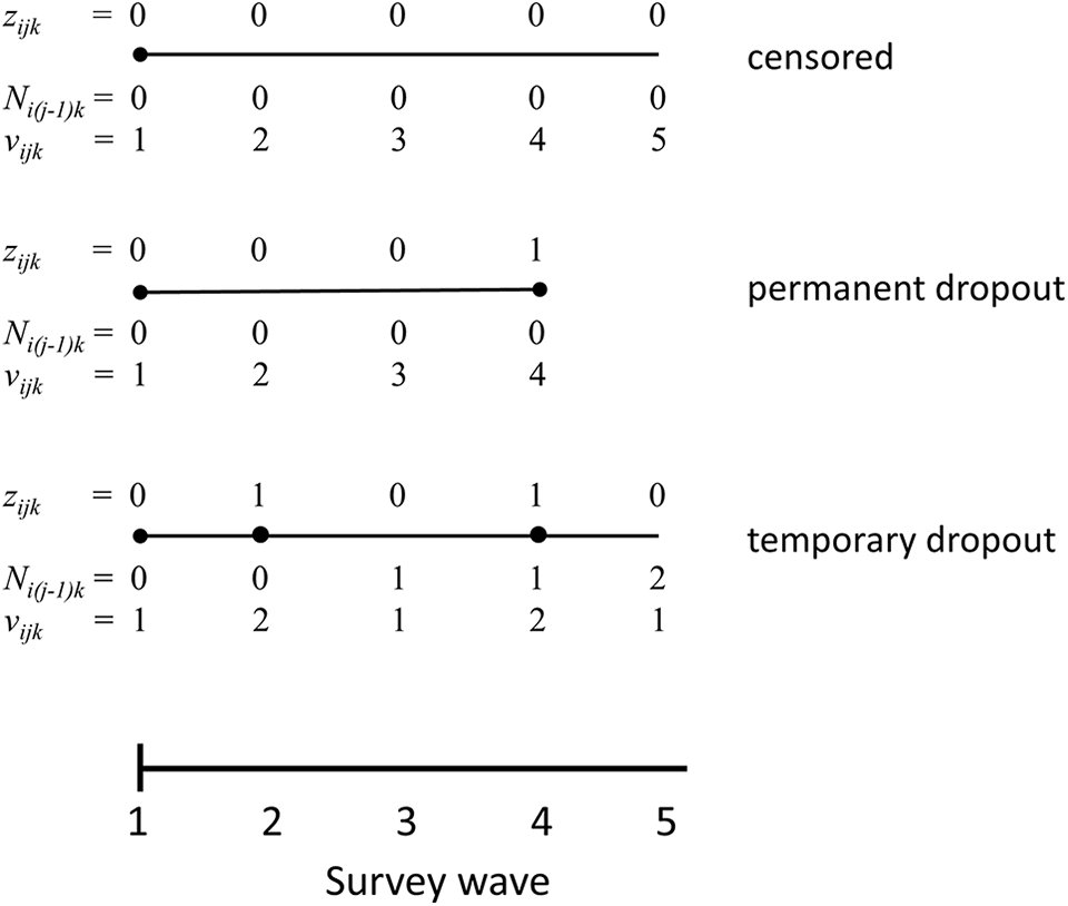
Let t_j represent the distinct event times (i.e., the T survey waves), n_i the number of time points observed for respondent i, and $δ_{i j} \in \{0, 1, ..., K\}$ the censoring indicator for respondent i at time t_j (with $j \in [0, T - 1]$ ) that distinguishes nonevents (δ _ij = 0) from events (δ _ij > 0). In our application, nonevents correspond to survey participation, whereas K equals 2 and reflects the two types of nonresponse (i.e., temporary and permanent dropout). The response variable Z is a stacked vector given by $z_{i j k} = I (δ_{i j} = k)$ with $k \in \{0, 1, ..., K\}$ and $j \in \{1, ..., n_{i}\}$ (see Figure 2). The probability of observing event k for respondent i between t_j₋₁ and t_j conditional covariates w_ij is modeled using a multinomial probit link as

Figure 2.

Outcome coding for different event types.

p_{i j k} = P (z_{i j k} = 1 | w_{i j}) = Φ [\sum_{l = 1}^{m} g (x_{i j} = [t_{j}, w_{i j}, v_{i j k}, N_{i (j - 1) k}]; T_{l}, M_{l})],

where Φ[·] is the standard normal distribution. Given the independent risks assumption, Equation(6) can also be specified in the form of multiple survival models with a binomial probit link (Sparapani et al., 2020), thus estimating Equation (6) independently for each event type k. The covariates x_ij include the event time t_j and (time-invariant) predictor variables w_ij. In addition, we acknowledge the exposure time v_ijk of respondent i at t_j, that is, the number of discrete time points since the beginning of the episode for event k. Finally, the covariates also comprise N_i_(j−1)k, that is, the number of events of type k previously observed up to the preceding event time t_j₋₁. For a single (K = 1), nonrecurring event, v_ijk is identical for all observation units and N_i_(j−1)k = 0 because all individuals have the same study start time and units that have already experienced an event are no longer part of the risk set. Thus, v_ijk and N_i_(j−1)k are not needed in statistical modeling. Under these conditions, our model reduces to the BART survival model introduced by Sparapani and colleagues (2016). In other words, our event history approach can be viewed as a generalization of the survival model for competing and possibly recurrent events.

The BART specification of Equation (6) places priors p(T_l) on the tree structure and p(μ _bl |T_l) on the terminal node values given the tree structure as described above. Then, samples can be generated from the posteriori distribution for any event time t_j and event type k to obtain the posterior distribution p_jk. These samples can be used to approximate any conceivable distribution of individual and group statistics such as individual participation probabilities or the average dropout propensity of a group of individuals at a certain point in time.

Prediction of Unconditional Response Rates

From a BART event history model, values of Z can be predicted from the covariates w for future survey waves or for new values of w, for example, to evaluate expected response rates in a new panel study. Thus, along with the definition of Rubin (1976), the missing mechanism assumed here is missing at random (MAR). These predictions can be used to estimate nonresponse probabilities for the recurrent or nonrecurrent events included in the model at each survey wave t_j. Importantly, these estimates represent conditional probabilities given survival to t_j (i.e., given no permanent dropout). Combining the nonresponse probabilities for recurrent and nonrecurrent events using standard rules of probability theory also allows estimating the unconditional response probability at a given wave, thus estimating the expected sample size in a survey wave.

Formally, survey participation can be understood as a bivariate and time discrete, stochastic process (V_t, Z_t) with V_t representing survey participation resulting from a nonrecurrent event (i.e., permanent dropout) and Z_t the respective respondent outcome for a recurrent event (i.e., temporary dropout) at time point t. 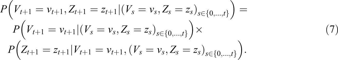Both processes can result in survey participation (PA) or nonresponse (NR), that is, $v_{t} \in \{P A, N R\}$ and $z_{t} \in \{P A, N R\}$ . This process is defined by its start distribution (V₀, Z₀) at the first survey wave and transition probabilities P(V_t+1 = v_t₊₁, Z_t+1 = z_t₊₁) given the previous states ${(V_{s} = v_{s}, Z_{s} = z_{s})}_{s \in \{0, ..., t\}} = (V_{0} = v_{0}, Z_{0} = z_{0}, ..., V_{t} = v_{t}, Z_{t} = z_{t})$ . The joint transition probabilities for V_t₊₁ and Z_t₊₁ can be derived from two submodels by splitting the respective probabilities into conditional probabilities for the nonrecurrent event (V_t₊₁) and the recurrent event (Z_t₊₁) in the following way (see the Supplemental Material for the full derivation of this decomposition):

\begin{array}{l} P (V_{t + 1} = v_{t + 1}, Z_{t + 1} = z_{t + 1} | {(V_{s} = v_{s}, Z_{s} = z_{s})}_{s \in \{0, ..., t\}}) = \\ P (V_{t + 1} = v_{t + 1} | {(V_{s} = v_{s}, Z_{s} = z_{s})}_{s \in \{0, ..., t\}}) \times \\ P (Z_{t + 1} = z_{t + 1} | V_{t + 1} = v_{t + 1}, {(V_{s} = v_{s}, Z_{s} = z_{s})}_{s \in \{0, ..., t\}}) . \end{array}

Note that in this decomposition, the transition probabilities for the nonrecurrent event (V_t₊₁) depend on the previous states ${(V_{s} = v_{s}, Z_{s} = z_{s})}_{s \in \{0, ..., t\}}$ , whereas the respective probabilities for the recurrent event (Z_t₊₁) are additionally conditioned on the current state of the recurrent event (V_t₊₁ = v_t₊₁). Each of these transition probabilities can be independently estimated using the BART event history approach in Equation (6) and, subsequently, combined to derive the unconditional nonresponse probability in a given wave t.

Consider the example in Figure 3 that describes the potential nonresponse sequences for three waves. In Wave 1 (t = 0), no nonresponse is observed. In Wave 2 (t = 1), the conditional probability of temporary $(p_{1}^{T D})$ or permanent dropout $(p_{1}^{P D})$ is estimated using Equation (6), resulting in an overall nonresponse probability of $p_{1}^{N R} = p_{1}^{P D} + [(1 - p_{1}^{P D}) \times p_{1}^{T D}]$ . Consequently, the unconditional probability of survey participation in Wave 2 is $p_{1}^{P A} = 1 - p_{1}^{N R}$ . For Wave 3 (t = 2), the calculation follows comparably, although also acknowledging the permanent dropout probability $p_{1}^{P D}$ from the previous wave. Thus, the unconditional nonresponse probability in Wave 3 is estimated as $p_{2}^{N R} = p_{1}^{P D} + (1 - p_{1}^{P D}) \times p_{2}^{T D} + (1 - p_{1}^{P D}) \times [(1 - p_{2}^{P D}) \times p_{2}^{T D}]$ . This logic can be continued to estimate the participation probabilities for any following survey wave. Moreover, it can also be easily extended to acknowledge additional types of nonresponse. For example, permanent dropout might be a consequence of dwindling motivations, and thus, the respondent’s active refusal to continue participation in a panel study. However, it might also result from an inability to contact the respondent because they moved without leaving valid contact information. In this case, a sequence of three types of nonresponse could be modeled, resulting in a three-step process.

Figure 3.

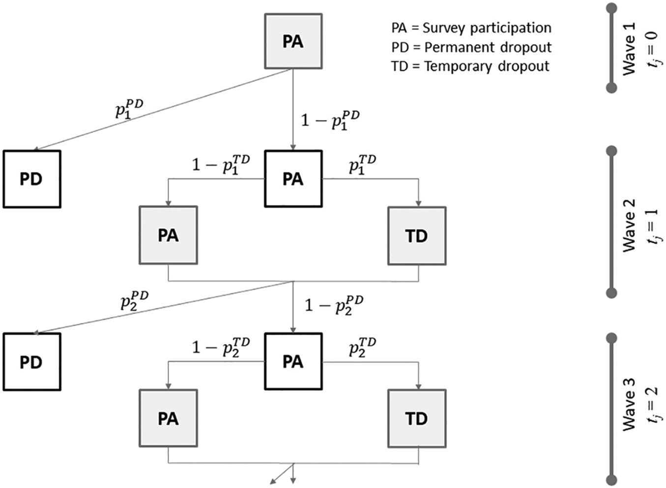
Two-step process of survey participation for two types of nonresponse across three waves.

This Study

The study examines nonresponse in the German National Educational Panel Study (NEPS; Blossfeld et al., 2011) that studies trajectories of competence development across the life course. We will demonstrate how to model participation rates across several measurement occasion using event history models that account for competing risks (i.e., participation vs. temporary dropout vs. permanent dropout). This enables us to elucidate unique predictors for each type of nonresponse. Moreover, using a BART for model estimation (Chipman et al., 2010), we avoid parametric or semiparametric constraints on the underlying model structure. This allows for the inclusion of large sets of predictor variables with complex interaction patterns and, thus, makes use of substantially more information than typical attrition analyses (e.g., using logistic regression models).

Method

Sample and Procedure

The participants are part of the NEPS (Blossfeld et al., 2011) that follows representative samples of German students across their school careers. For this study, we focus on a sample of N = 4,559 students (48% girls) that were initially surveyed in Grade 5 (year 2010). Subsequent measurements occurred each year until Grade 9 (year 2014), resulting in five measurement waves. The students attended various schools from rural and urban regions in Germany (see Steinhauer et al., 2015 for details on the sampling procedure): About 38% attended general or intermediate secondary schools (“Hauptschule/Realschule”), 50% went to higher secondary schools (“Gymnasium”), and the remaining 12% encompassed students from several specialized school branches. The mean age in Grade 5 was M = 15.13 years (SD = 0.51). More information on the data collection process including the interviewer selection and training is summarized on the project website (https://www.neps-data.de).

Measures

Survey participation

A respondent’s participation status was recorded at each wave as either participation, temporary dropout, or permanent dropout. In Grade 5, all students participated; thus, no dropout was observed. Permanent dropout was defined as an active refusal to further participate in the study or an inability to participate. It occurred for different reasons such as refusal of a school to participate in the NEPS, refusal of a student within an eligible school, or students switching to another school not included in the NEPS. We did not distinguish the different types of permanent dropout in our analyses because the respective numbers of cases for each category were rather small. In contrast, temporary dropout referred to nonparticipation at a given wave that was not due to permanent dropout.

Conditioning variables

A total of 77 variables were used to predict nonresponse at each survey wave. These variables had been previously used in nonresponse analyses (e.g., Zinn et al., 2018) or were expected to be related to survey participation. Most variables were included as respondent characteristics (e.g., sex) and also aggregated to the school level (e.g., percentage of female students) to acknowledge individual and context effects. All variables were measured in the first survey wave or before. Respondent characteristics included the age (in years), sex (0 = male, 1 = female), migration background (0 = no, 1 = yes), mother tongue (0 = German, 1 = other), household size (as number of people), and the number of books at home (1 = 0–10 books to 6 = more than 500 books) as an indicator of cultural capital (Sieben & Lechner, 2019). Moreover, as more specific student characteristics, we recorded whether a student had ever repeated a school year (0 = no, 1 = yes), the number of missed school days due to being sick, and the grades in German and mathematics (1 = very good to 6 = failing). We also considered various self-reported psychological characteristics: Satisfaction with life, current living standards, health, family, friends, and school were each measured with a single item on 11-point response scales from 0 (completely dissatisfied) to 10 (completely satisfied), subjective health was measured with a single item on a 5-point scale from 1 (very good) to 5 (very bad), self-esteem was captured with 10 items (ω_categorical = .86) from Rosenberg (1965) on 5-point response scales from 1 (does not apply at all) to 5 (applies completely), and self-concept in German (ω_categorical = .75), mathematics (ω_categorical = .89), and school (ω_categorical = .82) was each measured with 3 items on 4-point rating scales from 1 (does not apply at all) to 4 (applies completely). In addition, six cognitive measures were considered: Perceptual speed (Lang et al., 2014) and reading speed (Zimmermann et al., 2012) were each measured as sum scores across 93 and 51 items, respectively. Figural reasoning was captured with a Raven-type test as a sum score across 12 items (ω_categorical = .68; Lang et al., 2014). Orthography (Rel.¹ = .96; Blatt et al., 2017), mathematical competence (Rel.¹ = .80; Duchhardt & Gerdes, 2012), and reading competence (Rel.¹ = .81; Pohl et al., 2012) were each represented by an item response score based on 30, 25, or 33 items, respectively. School characteristics included the school type in the form of two dummy-coded variables for “intermediate secondary schools” and “other school types” (reference category: “higher secondary school”), the number of students and classes in Grade 8 as indicators of school size, the type of institution (0 = public, 1 = private), and two dummy-coded variables for the school location as “part urban/part rural” and “rural” (reference category: “urban”). Moreover, all respondent, student, and psychological characteristics were aggregated to the school level to indicate respective contextual influences. Finally, we considered the federal state in Germany as 15 dummy-coded indicators.

Statistical Analyses

Longitudinal nonresponse was analyzed across five waves using the nonparametric event history approach described above. The BART model specified 300 trees using α = .95 and β = 2 for the regularization prior p(T_j) and l = 3 and k = 2 for the prior p(μ _bj |T_j). That way we followed the recommendations of Chipman and colleagues (2010) for the specification of the prior distributions. The Bayesian estimation used 500 burn-in samples, a thinning of 500 draws in the MCMC algorithm, and 5,000 draws from the posterior distribution for the permanent and temporary dropout propensities at each wave and each respondent. Convergence was evaluated by means of visual inspections of autocorrelation and trace plots. Moreover, the Geweke’s (1992) statistic was examined by the posterior sample of 10 (arbitrarily chosen) individuals. Missing values on the covariates (see Supplemental Material) were imputed with the variable’s median. For covariates with missing rates, exceeding 5% additional dummy variables were created and included the prediction models.² The analyses were conducted in R Version 3.5.1 (R Core Team, 2018) using the BART package Version 2.2 (McCulloch et al., 2019).

We validated our approach by conducting two kinds of analyses. First, we performed an out-of-sample validation using two thirds of the total data as training data and one third as test data. The observed data were randomly assigned to the two subsets of data, the training and the test data. Then, we estimated the BART models outlined above based on the training data and predicted wave-specific probabilities of permanent and temporary dropout based on the test data. The predicted values were compared to the observed values in the test data. As a measure of accuracy, the percentage of values corresponding to the observed participation status in the test data was used. We repeated this process 5 times to guard against sampling bias. As a second form of validation, we estimated the BART models using the full data set but excluding the last survey wave. The last wave was used as test data. As before, we predicted for all individuals who were still at risk in the last wave their probabilities of permanently and temporarily dropping out. Again, the percentage of values that coincided between prediction and observation served as a measure of accuracy. Both types of validation are state of the art when dealing with models of statistical learning such as BART (e.g., Kern et al., 2019).

Finally, as a proof of concept, we compared the results of our BART models to results from comparable logistic regression models with least absolute shrinkage and selection operator (LASSO) penalization. Logistic regression models with LASSO are parametric models that are typically used for studying problems as the one addressed in this article (e.g., Pavlou et al., 2015). These models were validated in the same way as the BART models.

Data Availability

Most of the data analyzed in this study are provided at https://doi.org/10.5157/neps:sc3:8.0.0. Due to German privacy laws, some school variables (e.g., type of institution or school location) cannot be made publicly available. The analyses syntax to reproduce our results can be found at https://github.com/bieneschwarze/bartfornonresponse.git.

Results

Nonresponse Rates Across Survey Waves

Across the five survey waves, nonresponse rates increased from 11% (Wave 2) to 36% (Wave 5). The percentage of temporary dropout was rather constant and fell at about 4% at each wave, whereas permanent dropout increased in an approximately linear fashion (see Table 1). In each survey wave, the increase in permanent dropout rates varied between 6% (Wave 2) and 10% (Wave 3). The reasons for permanent dropout were manifold. Many students dropped out involuntarily because they switched to another school or, in later waves, left the school system altogether (e.g., starting a traineeship). The design of the NEPS implements a different (rather limited) survey program for these cases. Thus, we considered them permanent dropouts. Moreover, after the initial wave, some schools refused further participation in the NEPS, presumably, to avoid unduly disruptions of the school routines. In contrast, active refusals on part of the students were rather rare.

Table 1.

Nonresponse Across Survey Waves.

Participation status	Wave 1	Wave 2	Wave 3	Wave 4	Wave 5
Survey participation	4,559 (100%)	4,064 (89%)	3,606 (79%)	3,275 (72%)	2,905 (64%)
Temporary dropout	—	202 (4%)	201 (4%)	187 (4%)	214 (5%)
Permanent dropout	—	293 (6%)	752 (16%)	1,097 (24%)	1,440 (32%)
Student switched school		144 (3%)	432 (9%)	6 (0%)	—
Student left school system		—	—	924 (20%)	1,145 (25%)
Student refused		—	—	53 (1%)	203 (4%)
School refused		111 (2%)	219 (5%)	—	—
Unknown/other reasons		38 (1%)	96 (2%)	114 (3%)	92 (2%)
Total	4,559 (100%)	4,559 (100%)	4,559 (100%)	4,559 (100%)	4,559 (100%)

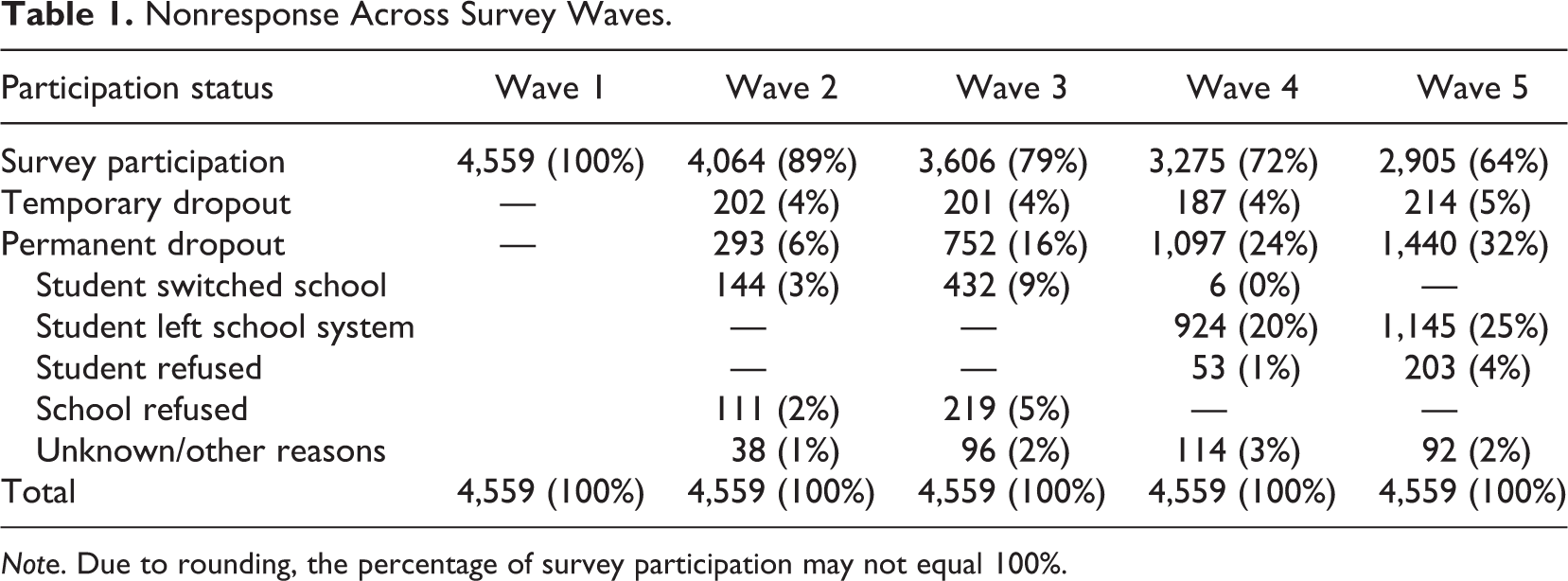
Note. Due to rounding, the percentage of survey participation may not equal 100%.

Prediction of Nonresponse Propensity

Predictors for two types of survey nonresponse (i.e., temporary and permanent dropout) in the NEPS were evaluated using BART event history modeling. The MCMC algorithm for these models converged satisfactorily. We observed no substantial autocorrelations in consecutive draws of the MCMC algorithm, and the trace plots indicated good mixing behavior of the distinct parts of the generated chain (see Supplemental Material). Moreover, Geweke’s (1992) tests showed no pronounced differences between the examined parts of the Markov chain. Thus, at this point, our BART approach worked well for the data. As a second step, we validated our models for survey nonresponse. Overall, our BART models performed well in predicting observed temporary and permanent dropout patterns for both types of validation criteria. All accuracy indices for the BART models ranged between 90% and 97% (see Table 2). With accuracies between 89% and 99%, the logistic regression models with LASSO performed similarly.³ These results show that neither approach seemed to outperform the other, at least not concerning the considered accuracy measure.

Table 2.

Accuracy Measure of Validation Studies.

Type of Validation	Wave-Specific Accuracy^a	Model for Permanent Dropout		Model for Temporary Dropout
Type of Validation	Wave-Specific Accuracy^a	BART	Logit With LASSO	BART	Logit With LASSO
Out of sample: overall waves	Wave 2	.95	.94	.95	.94
	Wave 3	.91	.89	.96	.99
	Wave 4	.93	.91	.96	.99
	Wave 5	.90	.89	.96	.98
Out of sample: only last wave	Wave 5	.90	.90	.97	.95

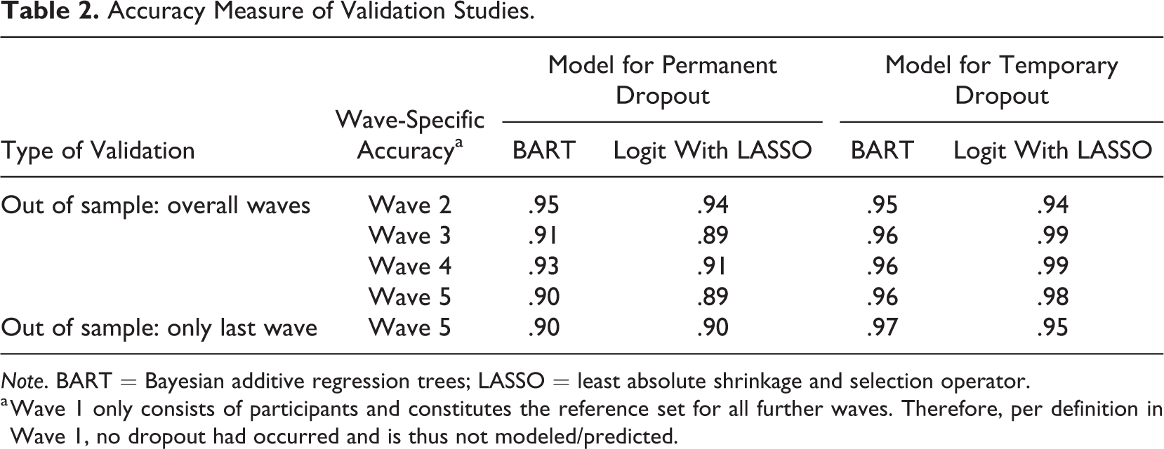
Note. BART = Bayesian additive regression trees; LASSO = least absolute shrinkage and selection operator.

^a Wave 1 only consists of participants and constitutes the reference set for all further waves. Therefore, per definition in Wave 1, no dropout had occurred and is thus not modeled/predicted.

Relative Variable Importance

The relative importance of the covariates for the trees of the BART models that predicted the nonrecurrent event (i.e., permanent dropout) is summarized in Figure 4 (complete results for all covariates are given in the Supplemental Material). Permanent dropout was primarily driven by the measurement occasion, that is, the survey wave: The time variable was chosen in about 26% of all trees. Interestingly, individual-level variables (i.e., respondent, student, and psychological characteristics) were rather uninformative for predicting permanent dropout. In contrast, context variables were more important. For example, the mean number of sick days (p_vi = .08), the mean grade in mathematics (p_vi = .05), or the mean subjective health (p_vi = .04) in the schools were relevant predictors of permanent dropout, whereas the respective respondent information was not. We received a slightly different picture for the prediction of temporary dropout. Figure 5 summarizes the results for covariates with an important contribution to a dropout event (full results are given in the Supplemental Material). Here, we found a strong impact of the students’ mean satisfaction with their health status on the school level (p_vi = .31), the mean number of students with migrations background at a school (p_vi = .14), and the number of books at home (p_vi = .10). The number of previous nonresponse events (p_vi = .07), the survey wave (p_vi = .03), the mean reading speed at school (p_vi = .07), the number of students in Grade 8 (as an indicator of school size; p_vi = .06), and the time without a participation event predicted temporary dropout as well, whereas further respondent and school context information did not as much. Together, these results highlight the importance of context information to predict nonresponse in large-scale assessments conducted in schools.

Figure 4.

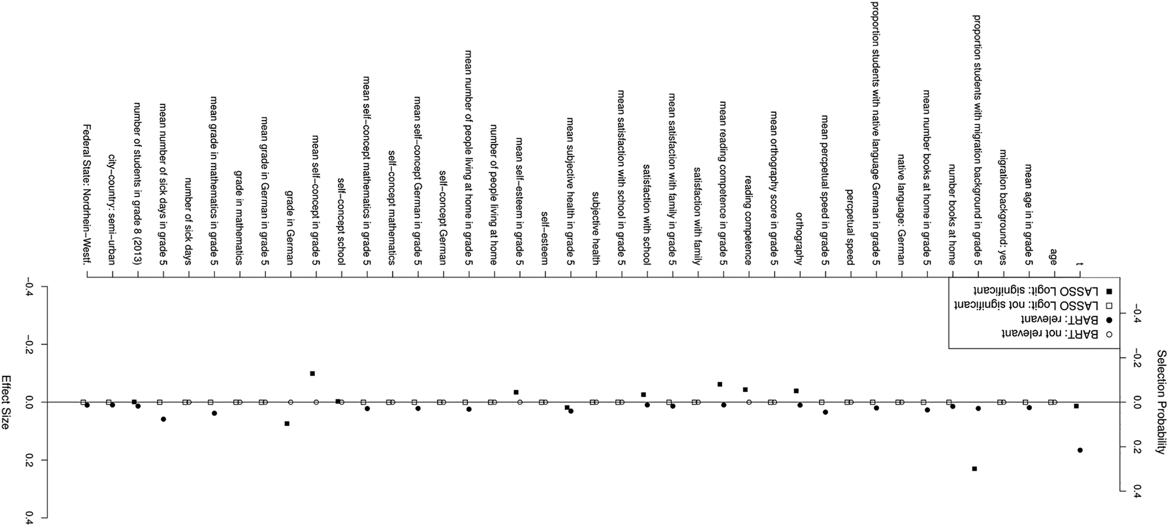
Relative importance of selected covariates for predicting permanent dropout with t as survey wave using Bayesian additive regression trees and least absolute shrinkage and selection operator regression. Note. The solid line represents the threshold for nonignorable importance, filled dots mark variables of nonignorable importance with significant impact (p < .05), and empty dots mark variables of ignorable importance with nonsignificant impact (p > .05). Full results are given in the Supplemental Material.

Figure 5.

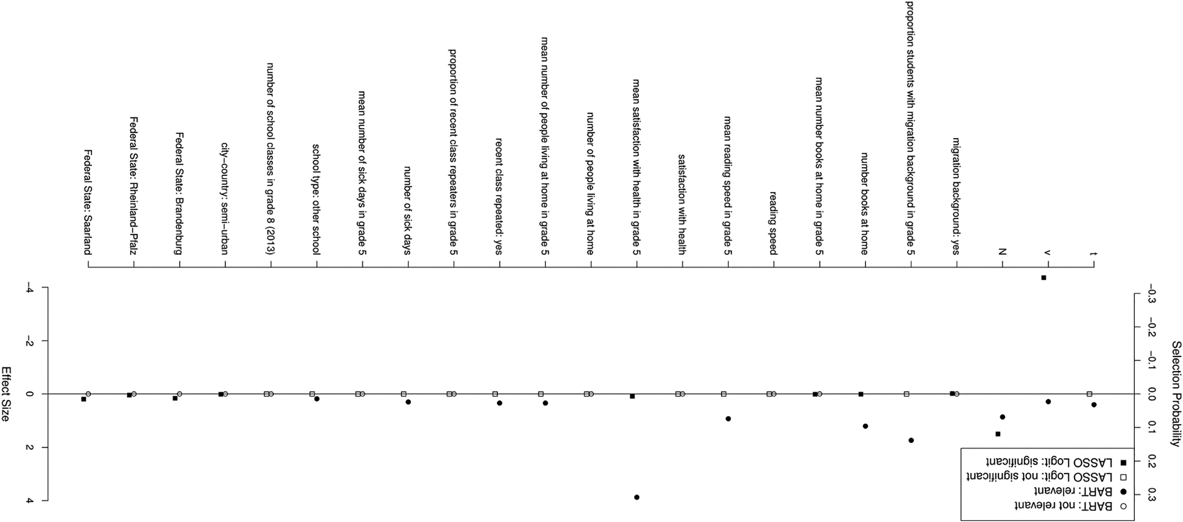
Relative importance of selected covariates for predicting temporary dropout with t as survey wave, v as the event time, and N as the number of previous dropouts for Bayesian additive regression trees and least absolute shrinkage and selection operator regression. Note. The solid line represents the threshold for nonignorable importance, filled dots mark variables of nonignorable importance with significant impact (p < .05), and empty dots mark variables of ignorable importance with nonsignificant impact (p < .05). Full results are given in the Supplemental Material.

Interestingly, logistic regression models with LASSO identified rather different covariates predicting dropout as BART (see Figures 4 and 5). For example, the BART model found the survey wave to be the most important factor triggering permanent dropout, whereas the LASSO regression identified the proportion of students with migration background as the driving force. BART also uncovered several important covariates that played no role according to LASSO regression (e.g., mean number of sick days in Grade 5, mean grade in mathematics in Grade 5). On the other hand, the logistic regression model considered a student’s German grade to be relevant for their permanent dropout propensity, which seemed to be completely irrelevant according to the BART model. Similar discrepancies were observed for the prediction of temporary dropout. Whereas BART identified the mean satisfaction with health and the proportion of students with migration background as the most important factors, LASSO regression highlighted the waves already spend in the study (i.e., the sojourn time per wave) and the total number of waves participating in the study. Again, most factors found relevant according to BART (e.g., number of books at home and mean reading speed in Grade 5) were not marked to be essential by LASSO regression (and vice versa). In order to assess whether multicollinearity causes the differences between the predictor sets identified as important by the two approaches, we examined the correlations and variance inflation factors between all predictors. As expected, some predictors were substantially correlated (e.g., the cognitive measures or grades). However, none of the important predictors identified by the BART models or the LASSO regressions showed substantial multicollinearity. We conclude from this finding that multicollinearity is not the driving force behind the observed differences. Instead, we find it very likely that the differences are caused by higher level interactions that BART considers, but LASSO does not. Thus, this is a clear argument for the trustworthiness of BART results.

Prediction of Participation Rates

The BART event history models allow predicting the participation rates at any survey wave (potentially, even beyond the observational period of the study) given the observed covariates. Importantly, these represent conditional probabilities dependent that no permanent dropout has occurred in the previous waves. Panel A in Figure 6 summarizes the conditional probability distributions of permanent dropout of all individuals in Waves 2–5. These results show that the conditional probabilities of permanent dropout were on average about 6.6% with a 95% credibility interval (CI) of [5.9%, 7.2%] in Wave 2 and increased to 10.0%, 95% CI [9.1%, 10.9%] in Wave 5. In contrast, the conditional probabilities of temporary dropout for the individuals who were at risk to experience such an event (Panel B in Figure 6) were nearly identical across the four survey waves. They were about 5.0%, 95% CI [4.4%, 5.6%], in Wave 2; 5.2%, 95% CI [4.7%, 5.7%], and 5.5%, 95% [4.8%, 6.0%], in the Waves 3 and 4; and 6.6%, 95% CI [5.6%, 7.5%], in Wave 5, respectively. Following the two-step process outlined above, we also estimated the unconditional response probabilities, that is, the expected participation rates at each wave (Panel C in Figure 6). These results show continually decreasing response rates in successive survey waves. Whereas a response rate of 88.8%, 95% CI [87.8%, 89.6%], was predicted for Wave 2, it decreased to 63.7%, 95% CI [62.3%, 65.0%], for Wave 5. Importantly, these model predicted participation rates closely reproduced the descriptive survey participation rates given in Table 1. Therefore, the BART event history model could be used to predict expected response rates beyond the observational period.

Figure 6.

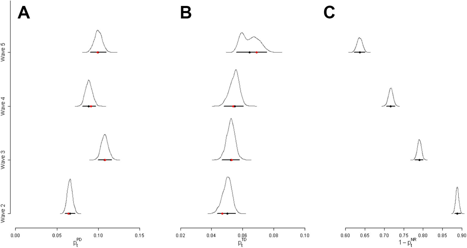
Predicted participation status across waves. (A) Conditional permanent dropout rates, (B) Conditional temporary dropout rates, and (C) Unconditional participation rates. The black curves are the posterior densities of the estimated probabilities. The black dots mark their median, the horizontal lines their 95% credibility intervals, and the red dots in Panel A and B the empirical frequencies of the number of observed events.

Discussion

Machine learning methods offer intriguing opportunities for survey researchers in various contexts (Buskirk et al., 2018; Kern et al., 2019; Toth & Phipps, 2014). Particularly, tree-based approaches include a bundle of versatile alternatives to parametric regression that allow the modeling of complex relationships with computational efficiency. This article presented a recently introduced Bayesian ensemble method (Chipman et al., 2010) for the analysis of nonresponse in social surveys. In contrast to wave-to-wave predictions that dominated previous nonresponse research (e.g., Durrant & Steele, 2009), we focused on the analysis of survey participation across multiple waves. We developed a nonparametric BART event history model to analyze competing risks for different types of nonresponse, that is, temporary and permanent dropout. This modeling strategy enables researchers to identify important variables driving the nonresponse process and, more importantly, constructing longitudinal prediction models. We applied our novel approach to data from a German large-scale assessment and showed that nonresponse in longitudinal school-based studies is predominately driven by the school context (e.g., mean number of sick days and mean satisfaction with health) and to a lesser degree by student characteristics. As expected, nonresponse also increased throughout the survey with each wave. The model-implied nonresponse rates highlighted that permanent dropout increased from 6.6% to 10.0%, whereas temporary dropout was nearly constant across the survey waves. Using two types of validity criteria and a model comparison with logistic regression with LASSO, we were able to highlight the advantages of BART. For example, in our application, BART was able to predict the last wave’s response pattern using only information from previous waves. A notable strength of our BART modeling approach is its flexibility to acknowledge different nonresponse processes. Although our analyses were limited to temporary and permanent dropout, an extension to additional types of nonresponse is straightforward by adapting the outcome coding (see Figure 2). For example, it is advisable to distinguish active refusal to participate in a survey from a failure to contact the respondent. In this case, three competing events could be contrasted. Even structural breaks resulting from different contexts experienced by the respondents could explicitly be modeled. In our data example, a substantial proportion of students left the school system after Wave 3 (and, thus, turned into permanent dropout cases by design). Thus, more precise estimates of nonresponse trajectories might be derived by modeling different sequences of nonresponse, that is, before and after the anticipated structural break resulting from the different educational choices.

Implications for Survey Management

The presented nonresponse model can facilitate operational survey management in different ways. For example, prediction models can help to gauge expected sample sizes across the course of a panel study. If a valid prediction model can be established, the predicted response rates for upcoming survey waves can be used to plan sample refreshments or preestimate sample mortality (i.e., time frames for discontinuing further surveying). Alternatively, these analyses might also guide strategies to prevent nonresponse from taking place in the first place. If respondents with a high nonresponse probability can be identified beforehand, incentives might be adjusted accordingly (cf. Tourangeau et al., 2017). Adaptive incentivization strategies might even link the size of an incentive to the predicted probability of nonresponse (see Figure 7): Respondents that are expected to dropout are promised higher monetary compensations as compared to respondents with lower dropout propensities. Finally, if relevant characteristics of nonresponding units can be identified, these variables might guide sampling strategies for future surveys. Then, oversampling plans might be devised that explicitly target these subgroups with high propensity to dropout.

Figure 7.

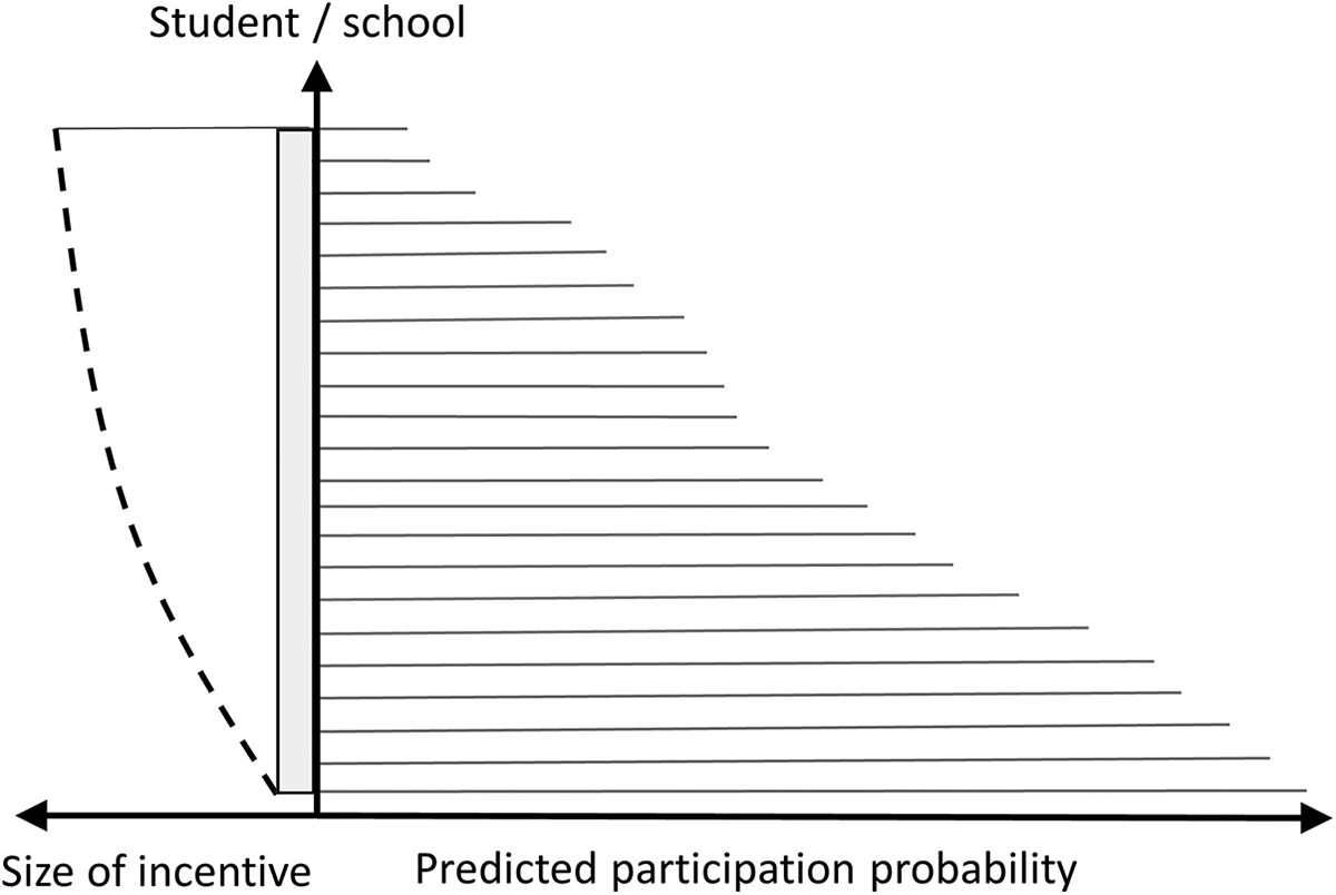
Example of an adaptive incentivization scheme dependent on predicted participation probabilities. The gray box represents the baseline incentive and the line represents dashed the additional incentive.

Limitations and Possible Extensions

Although the BART framework allows for complex modeling approaches, our event history model could be extended in several ways. For example, our predictor set was limited to information collected prior to or at the first measurement occasion. However, panel studies collect new information about respondents in each wave. A fruitful model extension pertains to the inclusion of time-varying covariates that are gathered during the course of a longitudinal study. Moreover, in the present form, our model considers only observed individual-specific heterogeneity. Although it can be assumed that the large number of predictors studied covers individual-specific heterogeneity on its whole, in the future, our approach could be extended by a frailty term. It would also be interesting to know how well our BART approach fares as compared to other machine learning methods such as random forests and boosted trees. Because the evaluation of their relative performance is beyond the scope of this study, it is an important undertaking left for future work. In a related vein, it might also be worthwhile to extend the scope of our BART approach and evaluate whether it is suitable for imputing missing values of time-to-event data. So far, studies have already highlighted the potential of BART for imputing MAR covariates (Xu et al., 2016) or for imputing MAR data in the context of augmented inverse probability estimation and penalized splines propensity prediction (Tan et al., 2019). The extension of these approaches to longitudinal data seems a worthwhile endeavor for future work. Finally, the generalizability of our findings on the predictors of dropout beyond the studied student sample should be an objective of further research. This would help to establish whether the identified predictors of nonresponse are similarly important in different populations (e.g., adults) and contexts (e.g., household surveys).

Conclusion

Modern machine learning techniques such as BARTs augment the statistical toolbox of survey researchers for nonresponse adjustments and the examination of nonresponse patterns. In longitudinal settings, BART prediction models facilitate the estimation of response rates in upcoming survey ways. For this purpose, this study described a novel event history approach that allows examining competing risks for different types of nonresponse. In an empirical demonstration, we showed that this technique allows identifying important drivers of temporary and permanent dropout across multiple survey waves. Thus, operational survey management might use respective prediction models to gauge sample mortality and plan sample refreshments at an early stage.

Supplemental Material

sj-docx-1-ssc-10.1177_0894439320928242 – Supplemental Material for Analyzing Nonresponse in Longitudinal Surveys Using Bayesian Additive Regression Trees: A Nonparametric Event History Analysis

Supplemental Material, sj-docx-1-ssc-10.1177_0894439320928242 for Analyzing Nonresponse in Longitudinal Surveys Using Bayesian Additive Regression Trees: A Nonparametric Event History Analysis by Sabine Zinn and Timo Gnambs in Social Science Computer Review

Footnotes

Authors’ Note

This article uses data from the National Educational Panel Study (NEPS): Starting cohort Grade 5, . From 2008 to 2013, NEPS data were collected as part of the Framework Program for the Promotion of Empirical Educational Research funded by the German Federal Ministry of Education and Research. As of 2014, NEPS is carried out by the Leibniz Institute for Educational Trajectories at the University of Bamberg in cooperation with a nationwide network.

Author Contributions

Both authors contributed equally to this work.

Data Availability

Most of the data analyzed in this study are provided at . Due to German privacy laws, some school variables (e.g., type of institution or school location) cannot be made publicly available.

Declaration of Conflicting Interests

The authors declared no potential conflicts of interest with respect to the research, authorship, and/or publication of this article.

Funding

The authors received no financial support for the research, authorship, and/or publication of this article.

Software Information

The analyses were conducted in R Version 3.5.1 using the BART package Version 2.2. The analyses syntax to reproduce our results are available at .

Supplemental Material

The supplemental material is available in the online version of the article.

Notes

Author Biographies

Sabine Zinn holds a PhD in computer science and statistics and is currently heading the Survey Management and Methodology Department of the Socio-Economic Panel (SOEP) at the German Institut for Economic Research (DIW) in Berlin (Germany). Her main research interests are computational statistics and survey methodology.

Timo Gnambs holds a PhD in psychology and is currently head of the research unit Educational Measurement at the Leibniz Institute for Edcuational Trajectories in Bamberg (Germany). His research includes methods of longitudinal large-scale assessments, technology-based psychological assessment, and meta-analyses.

References

Adams

R. J.

(2005). Reliability as a measurement design effect. Studies in Educational Evaluation, 31, 162–172. https://doi.org/10.1016/j.stueduc.2005.05.008

Adhikari

Bryant

L. A.

(2018). Sampling hard-to-locate populations. In Atkeson

L. R.

Alvaraz

R. M.

(Eds.), The Oxford handbook of polling and survey methods (pp. 155–180). Oxford University Press. https://doi.org/10.1093/oxfordhb/9780190213299.013.2

Beullens

Vandenplas

Loosveldt

Stoop

(2018). Response rates in the European Social Survey: Increasing, decreasing, or a matter of fieldwork efforts? Survey Methods: Insights from the Field. https://doi.org/10.13094/SMIF-2018-00003

Blatt

Jarsinski

Prosch

(2017). Technical report for orthography: Scaling results of starting Cohort 3 in Grades 5, 7, and 9 (NEPS Survey Paper No. 15). Leibniz Institute for Educational Trajectories.

Bleich

Kapelner

George

E. I.

Jensen

S. T.

(2014). Variable selection for BART: An application to gene regulation. The Annals of Applied Statistics, 8, 1750–1781. https://doi.org/10.1214/14-AOAS755

Blossfeld

H.-P.

Roßbach

H.-G.

von Maurice

(2011). Editorial. Zeitschrift für Erziehungswissenschaft, 14, 1–4. https://doi.org/10.1007/s11618-011-0198-z

Breiman

Friedman

Olshen

Stone

(1984). Classification and regression trees. Brooks/Cole Publishing.

Brüderl

Trappmann

(2017). Data collection in panel surveys. Methods, Data, and Analyses, 11, 3–6.

Buskirk

T. D.

Kirchner

Eck

Signorino

C. S.

(2018). An introduction to machine learning methods for survey researchers. Survey Practice, 11, 1–10. https://doi.org/10.29115/SP-2018-0004

10.

Buskirk

T. D.

Kolenikov

(2015). Finding respondents in the forest: A comparison of logistic regression and random forest models for response propensity weighting and stratification. Survey Methods: Insights from the Field. https://doi.org/10.13094/SMIF-2015-00003

11.

Chipman

H. A.

George

E. I.

McCulloch

R. E.

(1998). Bayesian CART model search (with discussion and a rejoinder by the authors). Journal of the American Statistical Association, 93, 935–960. https://doi.org/10.1080/01621459.1998.10473750

12.

Chipman

H. A.

George

E. I.

McCulloch

R. E.

(2010). BART: Bayesian additive regression trees. The Annals of Applied Statistics, 4, 266–298. https://doi.org/10.1214/09-AOAS285

13.

Díaz-Uriarte

de Andrés

A. S.

(2006). Gene selection and classification of microarray data using random forest. BMC Bioinformatics, 7, 1–13. https://doi.org/10.1186/1471-2105-7-3

14.

Duchhardt

Gerdes

(2012). NEPS technical report for mathematics—Scaling results of starting Cohort 3 in fifth grade (NEPS Working Paper No. 19). Otto-Friedrich-Universität Bamberg.

15.

Durrant

G. B.

Steele

(2009). Multilevel modelling of refusal and non-contact in household surveys: Evidence from six UK government surveys. Journal of the Royal Statistical Society: Series A, 172, 361–381. https://doi.org/10.1111/j.1467-985X.2008.00565.x

16.

Earp

Mitchell

McCarthy

J. S.

Kreuter

(2014). Modeling nonresponse in establishment surveys: Using an ensemble tree model to create nonresponse propensity scores and detect potential bias in an agricultural survey. Journal of Oficial Statistics, 30, 701–719. https://doi.org/10.2478/jos-2014-0044

17.

Felderer

Müller

Kreuter

Winter

(2018). The effect of differential Incentives on attrition bias: Evidence from the PASS wave 3 incentive experiment. Field Methods, 30, 56–69. https://doi.org/10.1177/1525822X17726206

18.

Geweke

(1992). Evaluating the accuracy of sampling-based approaches to the calculation of posterior moments. In Bernardo

J. M.

Smith

A. F. M.

Dawid

A. P.

Berger

J. O.

(Eds.), Bayesian statistics 4 (pp. 169–193). Oxford University Press.

19.

Gramacy

R. B.

Taddy

Wild

S. M.

(2013). Variable selection and sensitivity analysis using dynamic trees, with an application to computer code performance tuning. The Annals of Applied Statistics, 7, 51–80. https://doi.org/10.1214/12-AOAS590

20.

Hastie

Tibshirani

(2000). Bayesian backfitting (with comments and a rejoinder by the authors). Statistical Science, 15, 196–223. https://doi.org/10.1214/ss/1009212815

21.

Heffetz

Reeves

D. B.

(2019). Difficulty of reaching respondents and nonresponse bias: Evidence from large government surveys. The Review of Economics and Statistics, 101, 176–191. https://doi.org/10.1162/rest_a_00748

22.

Kapelner

Bleich

(2016). BartMachine: Machine learning with Bayesian additive regression trees. Journal of Statistical Software, 70, 1–40. https://doi.org/10.18637/jss.v070.i04

23.

Keiding

(2014). Event history analysis. Annual Review of Statistics and Its Application, 1, 333–360. https://doi.org/10.1146/annurev-statistics-022513-115558

24.

Kern

Klausch

Kreuter

(2019). Tree-based machine learning methods for survey research. Survey Research Methods, 13, 73–93. https://doi.org/10.18148/srm/2019.v1i1.7395

25.

Kleinert

Christoph

Ruland

(2019). Experimental evidence on immediate and long-term consequences of test-induced respondent burden for panel attrition. Sociological Methods & Research. Advance online publication. https://doi.org/10.1177/0049124119826145

26.

Kreuter

(2013). Facing the nonresponse challenge. Annals of the American Academy of Political and Social Science, 64, 23–35. https://doi.org/10.1177/0002716212456815

27.

Kuhn

Johnson

(2013). Applied predictive modeling. Springer.

28.

Lang

F. R.

Kamin

Rohr

Stünkel

Williger

(2014). Erfassung der fluiden kognitiven Leistungsfähigkeit über die Lebensspanne im Rahmen des Nationalen Bildungspanels: Abschlussbericht zu einer NEPS-Ergänzungsstudie [Measurement of fluid cognitive abilities over the life course in the NEPS] (NEPS Working Paper No. 43). Leibniz-Institut für Bildungsverläufe, Nationales Bildungspanel.

29.

McCulloch

Sparapani

Gramacy

Spanbauer

Pratola

(2019). BART: Bayesian additive regression trees (R package Version 2.2. https://CRAN.R-project.org/package?=BART

30.

McGovern

M. E.

Canning

Bärnighausen

(2018). Accounting for non-response bias using participation incentives and survey design: An application using gift vouchers. Economics Letters, 171, 239–244. https://doi.org/10.1016/j.econlet.2018.07.040

31.

Michaud

P. C.

Kapteyn

Smith

J. P.

van Soest

(2011). Temporary and permanent unit non-response in follow-up interviews of the health and retirement study. Longitudinal and Life Course Studies, 2, 145–169. https://doi.org/10.14301/llcs.v2i2.114

32.

Mills

(2011). Introducing survival and event history analysis. Sage.

33.

Müller

Castiglioni

(2020). Do temporary dropouts improve the composition of panel data? An analysis of “Gap Interviews” in the German Family Panel pairfam. Sociological Methods & Research, 49, 193–215.

34.

Pavlou

Ambler

Seaman

S. R.

Guttmann

Elliott

King

Omar

R. Z.

(2015). How to develop a more accurate risk prediction model when there are few events. BMJ, 351, h3868. https://doi.org/10.1136/bmj.h3868

35.

Peytchev

(2009). Survey breakoff. Public Opinion Quarterly, 73, 74–97. https://doi.org/10.1093/poq/nfp014

36.

Phipps

Toth

(2012). Analyzing establishment nonresponse using an interpretable regression tree model with linked administrative data. The Annals of Applied Statistics, 6, 772–794. https://doi.org/10.1214/11-AOAS521

37.

Pohl

Haberkorn

Hardt

Wiegand

(2012). NEPS technical report for reading—Scaling results of starting Cohort 3 in fifth grade (NEPS Working Paper No. 15). Otto-Friedrich-Universität Bamberg.

38.

R Core Team. (2018). R: A language and environment for statistical computing. R Foundation for Statistical Computing. https://www.R-project.org

39.

Rosenberg

(1965). Society and the adolescent self-image. Princeton University Press.

40.

Roßmann

Gummer

(2016). Using paradata to predict and correct for panel attrition. Social Science Computer Review, 34, 312–332. https://doi.org/10.1177/0894439315587258

41.

Rubin

D. B.

(1976). Inference and missing data. Biometrika, 63, 581–592. https://doi.org/10.1093/biomet/63.3.581

42.

Sieben

Lechner

C. M.

(2019). Measuring cultural capital through the number of books in the household. Measurement Instruments for the Social Sciences, 2, 1. https://doi.org/10.1186/s42409-018-0006-0

43.

Sparapani

R. A.

Logan

B. R.

McCulloch

R. E.

Laud

P. W.

(2016). Nonparametric survival analysis using Bayesian additive regression trees (BART). Statistics in Medicine, 35, 2741–2753. https://doi.org/10.1002/sim.6893

44.

Sparapani

R. A.

Logan

B. R.

McCulloch

R. E.

Laud

P. W.

(2020). Nonparametric competing risks analysis using Bayesian additive regression trees. Statistical Methods in Medical Research, 29, 57–77. https://doi.org/10.1177/0962280218822140

45.

Steinhauer

H. W.

Aßmann

Zinn

Goßmann

Rässler

(2015). Sampling and weighting cohort samples in institutional contexts. AStA Wirtschafts- und Sozialstatistisches Archiv, 9, 131–157. https://doi.org/10.1007/s11943-015-0162-0

46.

Tan

Y. V.

Flannagan

C. A.

Elliott

M. R.

(2019). “Robust-squared” imputation models using BART. Journal of Survey Statistics and Methodology, 7, 465–497. https://doi.org/10.1093/jssam/smz002

47.

Toth

Phipps

(2014). Regression tree models for analyzing survey response. In Proceedings of the government statistics section (pp. 339–351). American Statistical Association. https://www.bls.gov/osmr/research-papers/2014/st140160.htm (accessed 18 May 2020).

48.

Tourangeau

Brick

M. J.

Lohr

(2017). Adaptive and responsive survey designs: A review and assessment. Journal of the Royal Statistical Society: Series A, 180, 203–223. https://doi.org/10.1111/rssa.12186

49.

Trappmann

Gramlich

Mosthaf

(2015). The effect of events between waves on panel attrition. Survey Research Methods, 9, 31–43. https://doi.org/10.18148/srm/2015.v9i1.5849

50.

van Buuren

(2018). Flexible imputation of missing data. CRC Press.

51.

van Smeden

Moons

K. G.

de Groot

J. A.

Collins

G. S.

Altman

D. G.

Eijkemans

M. J.

Reitsma

J. B.

(2019). Sample size for binary logistic prediction models: Beyond events per variable criteria. Statistical Methods in Medical Research, 28, 2455–2474.

52.

Voorpostel

Lipps

(2011). Attrition in the Swiss Household Panel: Is change associated with later drop-out? Journal of Official Statistics, 27, 301–318.

53.

Watson

Wooden

(2014). Re-engaging with survey non-respondents: Evidence from three household panels. Journal of the Royal Statistical Society: Series A, 177, 499–522. https://doi.org/10.1111/rssa.12024

54.

West

B. T.

(2013). An examination of the quality and utility of interviewer observations in the National Survey of Family Growth. Journal of the Royal Statistical Society: Series A, 176, 211–225. https://doi.org/10.1111/j.1467-985X.2012.01038.x

55.

Williams

Brick

J. M.

(2017). Trends in U.S. face-to-face household survey nonresponse and level of effort. Journal of Survey Statistics and Methodology, 6, 186–211. https://doi.org/10.1093/jssam/smx019

56.

Daniels

M. J.

Winterstein

A. G.

(2016). Sequential BART for imputation of missing covariates. Biostatistics, 17, 589–602. https://doi.org/10.1093/biostatistics/kxw009

57.

Zimmermann

Gehrer

Artelt

Weinert

(2012). The assessment of reading speed in Grade 5 and Grade 9. University of Bamberg.

58.

Zinn

Gnambs

(2018). Modeling competence development in the presence of selection bias. Behavior Research Methods, 50, 2426–2441. https://doi.org/10.3758/s13428-018-1021-z

59.

Zinn

Würbach

Steinhauer

H. W.

Hammon

(2018). Attrition and selectivity of the NEPS starting cohorts: An overview of the past 8 years (NEPS Survey Paper No. 35). Leibniz Institute for Educational Trajectories.

Supplementary Material

Please find the following supplemental material available below.

For Open Access articles published under a Creative Commons License, all supplemental material carries the same license as the article it is associated with.

For non-Open Access articles published, all supplemental material carries a non-exclusive license, and permission requests for re-use of supplemental material or any part of supplemental material shall be sent directly to the copyright owner as specified in the copyright notice associated with the article.

0.00 MB

2.05 MB