
Abstract
In this article, survey, sensor, and administrative data are combined to correct for survey point estimate bias due to underreporting. The response to the Dutch Road Freight Transport Survey is linked to records from a road sensor network consisting of automated weighing stations installed on highways in the Netherlands. Capture–recapture (CRC) methods are used to estimate underreporting in the survey. Heterogeneity of the vehicles with respect to capture and recapture probabilities is modeled through logistic regression and log-linear models. Six different estimators are discussed and compared. Results show a downward bias in the survey estimate due to underreporting, whereas the CRC estimators yield larger estimates. This research is a new example of multisource statistics, a promising approach to improve the benefits of sensor data in the field of official statistics.
Keywords
Introduction
Recently, nonprobability-based big data sources have become increasingly popular in social science research and official statistics. Due to their unknown data generating processes, these data sets are rarely used in the production of official statistics. However, in practice, it is often required to use this kind of data to provide statistics cheaper and faster and to reduce response burden (Buelens, 2012; Daas, Puts, Buelens, & van den Hurk, 2015). In most cases, big data sources are partial observations of one or few variables of a subset of a population (Buelens, Daas, Burger, Puts, & van den Brakel, 2014). One important type of big data is often produced and collected by sensors, which can be any device storing information about physical elements and human behavior (Ganguly, Gama, Omitaomu, Gaber, & Vatsavai, 2009). Sensor data are often not collected for research purposes (Connelly, Playford, Gayle, & Dibben, 2016). Rather, the resulting data sets are large, complex, and unsystematic. Finally, the data are often held by commercial agencies (Schnell, 2019). Nevertheless, the information the data hold should be utilized in the production of official statistics (Citro, 2014; Lohr & Raghunathan, 2017). A current promising concept seems to be the production of “multisource statistics” (De Waal, van Delden, & Scholtus, 2017). For these concepts, record linkage on a microlevel is an essential tool (Schnell, 2016), since big data sources often contain only a few or no covariates, resulting in a low information content.
When a sensor and a survey that independently measure an identical target variable can be linked by a unique identifier and can be enhanced with administrative data, a maximum information gain is achieved (Japec et al., 2015). In this case, the term “big data” can be expanded to “identifiable big data” (Shlomo & Goldstein, 2015). Hence, to evaluate the enhancement of survey data with administrative and big data, empirical research on linkable data sets is needed.
In this article, the Dutch Road Freight Transport Survey (RFTS), the weigh-in-motion (WIM) road sensor data, the Dutch Vehicle Register (BRV), and the Dutch enterprise register (ER) are linked on a microlevel for analysis.
An important aim of the RFTS is to provide estimates of transported shipment weight at quarterly and annual intervals. Due to nonresponse and underreporting, a downward bias in the RFTS point estimates is expected. We use WIM data to assess, quantify, and correct this bias associated with estimates of the number of days on which transport occurred and the corresponding transported shipment weights. The corrections are based on an application of CRC techniques. These techniques were originally developed in ecology and biology to estimate (unknown) population sizes. The RFTS and the WIM observations are considered as two capture occasions. The BRV and ER provide covariates to model heterogeneity in the capture probabilities both for RFTS and WIM. This application is a new example of multisource estimation in official statistics.
Research Background
The number of surveys conducted has increased over the last decades (Singer, 2016), while the nonresponse rates are increasing, too (Meyer, Mok, & Sullivan, 2015). Furthermore, surveys put an unnecessary burden on the respondent if the information of interest is accessible from other data sets (Schnell, 2015; Miller, 2017). Especially, time-based diary surveys collect data on specified time intervals and impose a heavy response burden. To reduce the effort of reporting, respondents may omit spells or may not respond at all. Correspondingly, those surveys yield low response rates (Krishnamurty, 2008). Accordingly, survey estimates might be biased downward due to “inaccurate reporting, nonreporting, and nonresponse” (Richardson, Ampt, & Meyburg, 1996). As will be shown, even in the case of a mandatory survey with a high response rate, these problems cannot be neglected.
The RFTS is a mandatory time-based diary survey collecting data from truck owners on road freight transport activities in a specified time interval. In the past, transport, mobility, and travel surveys were already subject to validation studies. For this purpose, GPS sensor data from portable devices have been analyzed with a geographic information system (GIS). However, these studies have important limitations. If no external sensor data can be linked to the survey, the potential respondents must participate in a supplementary survey. This additional burden results in very low participation rates (Bricka & Bhat, 2006). Additional issues arise from the fact that the data collection devices are connected to the survey unit (vehicle or person).
In practice, GPS devices cause problems due to intended or unintended switch off, delays due to standby mode, battery issues, or the device not being carried. Furthermore, the use of GPS devices in surveys is not suitable for all population members, for example, the elderly or retired (Bricka, Sen, Paleti, & Bhat, 2012). Finally, signal loss, signal noise, and matching of GPS and survey data complicate accurate measurements (Shen & Stopher, 2014).
Instead, data based on local, permanently installed road sensors are used in our research to validate and adjust survey estimates using CRC techniques. Hereby, the problems caused by respondent behavior as discussed above are avoided. To the best of our knowledge, road sensor data have not been used for correcting surveys before.
Literature on Underreporting in Transport, Mobility, and Travel Surveys
We limit the literature review to results based on randomly sampled surveys (n ≥ 1,000) of the general population in the field of transport, mobility, and travel. However, experiments with smaller samples will be reported as well.
In 1986, Hassounah, Cheah, and Steuart (1993) documented underreporting rates for a large-scale transportation survey in the United States varying regionally from 2.6% to 46.8%. Due to the technical absence of GPS data, this study used cordon counts to estimate underreporting. In GPS validation studies, vehicles were equipped with GPS devices to track movements. In the first GPS household travel survey (1997, United States), Pearson (2001) reported underreporting in trip rates of 12.4% and 31.1%. The discrepancy is due to the definition of dwell times. These findings were confirmed by Wolf, Oliveira, and Thompson (2003), who reported rates of missed trips up to 42% in the Californian Household Travel Survey. Bricka and Bhat (2006) summarized the levels of underreporting in GPS surveys in the United States and reported even higher rates up to 81%. Stopher, FitzGerald, and Xu (2007) reported contrary results for the Sydney Household Travel Survey (2004), where only 7.4% of trips were missed. However, all nonrecorded GPS trips due to technical issues were excluded. In recent studies, Bohte and Maat (2009) concluded that GPS-/GIS-based results from 2007 are comparable to results from the 2006 Dutch Travel Survey. In contrast, Wolf, Wilhelm, Casas, and Sen (2013) reported for a regional household travel survey in the United States (2010/2011) that GPS-based results showed higher trip rates. Summarizing the results for transport, mobility, and travel surveys, there seem to be contrary results but underreporting in reported trips is likely. Therefore, the use of sensor data to assess survey data quality and to validate and adjust biased survey estimates seems to be a promising method.
Data
Survey Data
The RFTS is conducted by Statistics Netherlands and is based on EUROSTAT (2016) guidelines. A central objective of the mandatory survey is to collect data on the weight of the shipments transported by Dutch trucks. Therefore, truck owners must report the days on which the truck was used and the corresponding shipment weight. No report is required if the truck was not used for transport purposes. The target population is the Dutch commercial vehicle fleet, excluding military, agricultural, and commercial vehicles older than 25 years. Furthermore, only vehicles with a weight of at least 3.5 tons and at least 2 tons of load capacity are taken into consideration. The sample is stratified by six variables (type of transport, type of vehicle, industry class, load capacity, age of vehicle, size of vehicle fleet) resulting in 74 strata. For each quarter of 2015, a separate sample is drawn and invited to the survey. A sampling unit consists of a truck license plate and a specific week for which reporting is required. Hence, a truck can be sampled more than once in 2015, but with different survey periods.
The RFTS is conducted using internet interviewing, postal interviewing, and querying of software-based journey planning systems. The latter is used by large haulers. Especially, small companies receive a paper questionnaire. All other haulers and truck owners are contacted by a postal letter and are invited to participate in a web survey.
The sample consists of 33,817 unique vehicle–week combinations. Of these, 3,597 cases are classified as nonresponse, resulting in a response rate of 89.4%. The answer categories regarding truck-related activities are the following: truck used (22,454), truck not used (5,304), and truck not owned (2,462). The latter case is defined as technical-nonresponse and is excluded from the analysis because the validity of the response cannot be verified. This is due to quarterly updates of the BRV, complexity in holding companies, vehicle rental, and vehicle leasing. However, in case of this response, the survey agency asks for contact information of the current owner. If this information is available, the current owner is contacted, and the original response is replaced by the new response. The answer category that the truck has not been used reduces the respondent’s burden considerably since only small parts of the questionnaire must be answered. Nevertheless, choosing this response fulfills the obligation to participate in the mandatory survey. It is expected to find cases of underreporting due to nonresponse and misreporting by falsely responding that the truck was not used. It is not possible to assess measurement errors due to the respondent reporting wrong dates the truck was used in the survey period or the respondent reporting the wrong weight of the transported shipment.
Road Sensor Data
The WIM road sensor network is operated by the Dutch national road administration. The purpose of this system is to detect overloaded trucks using a dynamic measurement while trucks pass the station. If there is suspicion of overloading, the truck is taken to a traffic checkpoint and a static weighting is done. In 2015, there were nine operating WIM systems. Six of the systems had two separate stations for each direction operating on one highway. The remaining three systems used one location to measure both directions (see Figure 1).
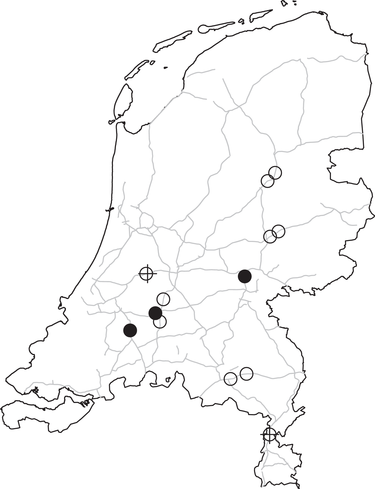
WIM road sensor stations on Dutch highways. The separate stations for each direction operating on one highway are shown with a circle. If they are close by, a cross is used 2 times to avoid overlapping circles. The filled dots count twice since they show the three systems where measures of both directions take place at the same location. WIM = weigh-in-motion.
This network installation results in 18 measurement points. For the analysis, the recorded variables are date, front/rear license plate, total weight, axles pressure, and automated truck classification. In 2015, a total of 35,669,347 trucks pass-by were recorded, of which 24,825,019 had a front license plate recognized by the WIM software system. Of those eligible, 3,733,064 records matched a truck from the survey using the front license plate as match variable, and 44,011 of the recorded trucks matched a truck in its corresponding survey period using the combination of time stamp (day) and front license plate as match variable.
For each truck, its axle weights are measured, and the total weight corresponds to the sum of the individual axle weights. Based on Enright and OBrien (2011) and expert information from the road administration, a conditional mean imputation was applied to the measured axles weights to correct for measurement errors. A deterministic error correction rule is used in this study. If the measured weight of an axle is greater than 20 tons, the weight of this axle is imputed by the average weight of the remaining axles. If the weight of more than one axle exceeds 20 tons, the average value of the remaining axles with a weight of less than 20 tons is used here, too. Due to 1,629 trucks having no axle weights stored in the data (the total weight is available), this rule could not be applied to these cases. Sensitivity analysis of the deterministic correction showed that choosing the threshold too small (≤15 tons) leads to a downward bias in the distribution of the measured weight. For these cases and cases where trucks were driving outside the speed interval (60–120 km/hr; see Enright & OBrien, 2011), the total weight was predicted using the technical characteristics from the vehicle register (described in paragraph “Administrative data”). Therefore, a stepwise model selection procedure based on the Bayesian information criterion (BIC) was applied (using R function “stepAIC” of the MASS package; Venables and Ripley [2002]) to select a model for a linear regression (r 2 adj. = 0.54).
In 17,321 of the 44,011 matched trucks (see the Results section), the trailer weight could not be linked to the WIM. This was due to the license plate not being recognized by the WIM software system (11,341) or the trailer not being registered in the vehicle register (5,980). The missing trailer weight was imputed with the mean of the empty trailer weight, conditional on the automated classification of the truck and its loading capacity.
Since the total weight measured includes the entire unit (truck, trailer, and shipment), the truck and trailer weights were subtracted using the weight information from the BRV. The resulting value corresponds to the transported weight, which is equal to the definition of reported weight in the RFTS.
The calculation of the transported shipment weight resulted in 3,945 negative values. These values were trimmed to 0 to not bias the estimate of the transported weight downward. Finally, an overall proportional bias correction was applied, calibrating the WIM-measured shipment weights to those reported in the RFTS. The correction factor was obtained from the subset of vehicles that were observed both in the RFTS and by WIM. This resulted in a downscaling of the WIM shipment weights by approximately 14%.
Administrative Data
The BRV and ER provide additional administrative data with information about technical truck characteristics and specifics of the truck owners. Both data sets were linked one by one to the RFTS and WIM data using the combination of license plate and the annual quarter as match variable.
The BRV contains the covariates, truck equipment class, type of fuel, number of wheels, number of cylinders, horsepower, emission class, maximum mass of truck, mass of empty truck, maximum mass of trailer, loading capacity, number of axles, width of truck, length of truck, leasing status, status of owner (person or company), province in which the owner is located, year of manufacture, and vehicle classification.
The covariates provided by the ER are the classification of economic activity (NACE), commercial or own transport, classification of company size, the size of the vehicle fleet, and the total fleet loading capacity. The variables of the BRV and ER will be used within the model selection to find appropriate covariates for the CRC models.
Approximately, 1% of the ER data and 0.008% of the BRV are missing. Observations with missing administrative data were excluded from the analysis (which explains the difference between the 44,011 matches [the Data section] and the 43,775 truck days in Table 1).
Captures of Truck Days in RFTS and WIM.
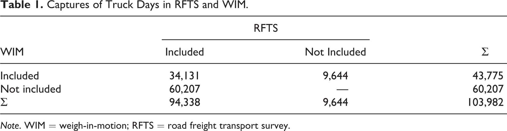
Note. WIM = weigh-in-motion; RFTS = road freight transport survey.
Method
Definitions and Notation
Each vehicle is in the survey for 1 week. Respondents must report all trips and shipments on each day.
We define the indicator
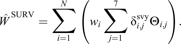
Survey Estimates
The regular, published outputs from the RFTS are poststratification estimates. Survey weights are computed, taking the survey design into account and correcting for selective nonresponse. The total of D and W is estimated by

with wi being the survey weight for vehicle i. The poststratification estimator for the total transported weight is given by
We will use bootstrap estimates for comparison with CRC techniques. Since the


This can be considered as a naive extended survey estimator, where WIM measurements are added to the survey response. This is the most basic way to include WIM and provides a lower bound on the more advanced estimators presented below.
CRC Methods
CRC techniques were originally developed to estimate the unknown size of an animal population (International Working Group for Disease Monitoring and Forecasting, 1995). These techniques were transferred to human populations and are frequently used in social and medical research to address undercounts in censuses, to estimate unknown population sizes, or to estimate the incidence of a disease (Böhning, van der Heijden, & Bunge, 2017). The biological procedure using traps to (re)capture animals is replaced by using at least two data sets containing elements of the target population. With two data sets A and B available, three quantities are derived: A\B, B\A, and A
Assumptions
In the present study, the population is assumed to be closed. There are no elements entering or leaving the population, making the unknown population size a constant. Since the percentage difference of vehicles listed in the BRV between the successive quarters and between the first and last quarter was <1%, this assumption is not severely violated. Furthermore, all elements used in this analysis belong to the population, as only Dutch trucks are in the RFTS, and the Dutch trucks in WIM can be identified by their license plate. The assumption of perfect linkage is met for trucks recognized by the WIM software system software as they can be linked one by one with their unique identifier of license plate and date. Since the WIM software system software failed occasionally to properly recognize a license plate, there might be more trucks which have been recorded in the survey period. Moreover, the inclusion of a truck in the RFTS is independent of the same truck being recorded by a WIM station (Chao, Tsay, Lin, Shau, & Chao, 2001). Finally, the capture probabilities for the elements should be homogeneous. However, it is sufficient if the homogeneity in capture probabilities is given for at least one data set (Van der Heijden, Cruyff, Whittaker, Bakker, & Smith, 2017). In the present study, the capture probabilities in the RFTS and WIM are modeled using covariates. Since the RFTS is a random sample survey, homogeneity conditional on the stratification variables can be assumed. By contrast, the inclusion of trucks in WIM is nonprobabilistic.
Lincoln–Petersen Estimator
The Lincoln–Petersen estimator (Lincoln, 1935; Petersen, 1893), also known as the dual-system estimator (Wolter, 1986), assumes homogeneous capture probabilities for all elements within every data set. This estimator uses the quantities
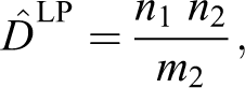
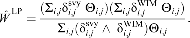
The estimator
Logit Model
Independently, Huggins (1989) and Alho (1990) proposed a likelihood approach, which is conditioned on the captured elements, to model heterogeneity in capture probabilities using covariates. The capture probabilities for each element on each occasion are modeled by means of a linear logistic model. We use covariates to model
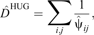

with

the estimated probability to be captured at least once, and
Log-Linear Model
Log-linear models for population size estimation in closed populations were introduced by Fienberg (1972). Two data sets A and B form an A × B contingency table with A\B, B\A, and A

Here,

This model has no interaction parameter and assumes the capture probabilities of A and B to be independent. It is denoted as
To model heterogeneity in the capture probabilities of A and B, any number of available covariates can be included in the model. Suppose the covariates X and Y are available, the two-way contingency table is expanded to a four-way contingency table:

The parameters
Model Selection
To select appropriate covariates to fit the logit and log-linear models, a stepwise selection procedure is used based on the BIC (using the “stepAIC” function). To cover the full information of the covariates, the model selection is based on the logit model, since the log-linear model only allows for categorical variables. In the logit model, all of the selected variables were used. In the log-linear model, the five variables with the most predictive power in the two logit models (see below) were combined. For that purpose, the continuous covariates were categorized based on their quantiles.
The first logit model uses
The second logit model uses
Variance Estimation
Bootstrapping is typically used to obtain variance estimates of model-based methods. For consistency and comparability, we computed bootstrap variance estimates for all estimators discussed. As mentioned earlier, this accounts for the cluster effects in the data due to the trucks being the sampling units and not the truck days. Hence, there are more truck days than sampling units. Further, the weight of the transported shipment is clustered in trucks.
Bootstrap samples are obtained from the original RFTS sample of trucks by simple random sampling with replacement. A bootstrap data set for estimation purposes consists of all records, both RFTS and WIM, that are available for the vehicles in the bootstrap sample. When the same vehicle is drawn more than once, all its associated records are repeated the number of times the vehicle occurs in the bootstrap sample.
The mean of the bootstrap distribution is computed to ascertain that the bootstrap procedure is unbiased. The variance of the bootstrap distribution is used as a variance estimate. The 0.025% and 0.975% quantiles of the bootstrap distribution are used to estimate the lower and upper boundaries of the 95% confidence intervals.
Linking RFTS and WIM
Table 1 shows the truck days of the matched RFTS and WIM. There were 94,338 truck days reported in the RFTS. 43,775 truck days were captured in the WIM, of which 34,131 were reported in the RFTS. On 9,644 days, there were no reported trips in the RFTS, but trucks were recorded at a WIM station. On 60,207 days, there were reported trips in the RFTS, but nothing was captured in the WIM.
Table 2 shows the matched data sets as well, but the cells include the transported shipment weight in kilotons (kt) on the reported truck days. In the RFTS, 953.71 kt were reported. In the WIM, 475.96 kt were captured in the WIM, of which 376.83 kt were reported in the RFTS. In the WIM, 99.13 kt were measured but were not reported in the RFTS. In the RFTS, 576.88 kt were reported which were not captured in the WIM.
Captures of Transported Shipment Weight (in kt) in RFTS and WIM.
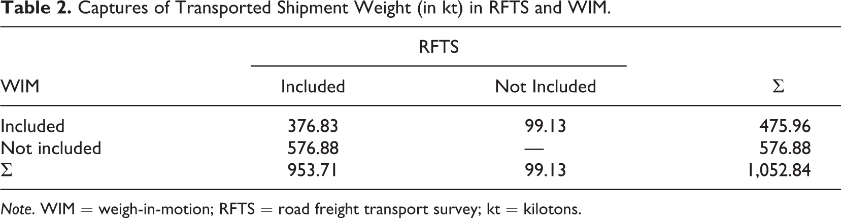
Note. WIM = weigh-in-motion; RFTS = road freight transport survey; kt = kilotons.
Results
All estimators applied show noticeable amounts of underreporting for truck days (Table 3; Figure 2, left panel) and transported shipment weight (Table 4; Figure 2, right panel) in the RFTS. However, the estimated amount of underreporting varies between the estimators. A similar pattern in the amount of underestimation is found for both two target variables. Table 3 and the left panel of Figure 2 show the results for the estimated truck days.
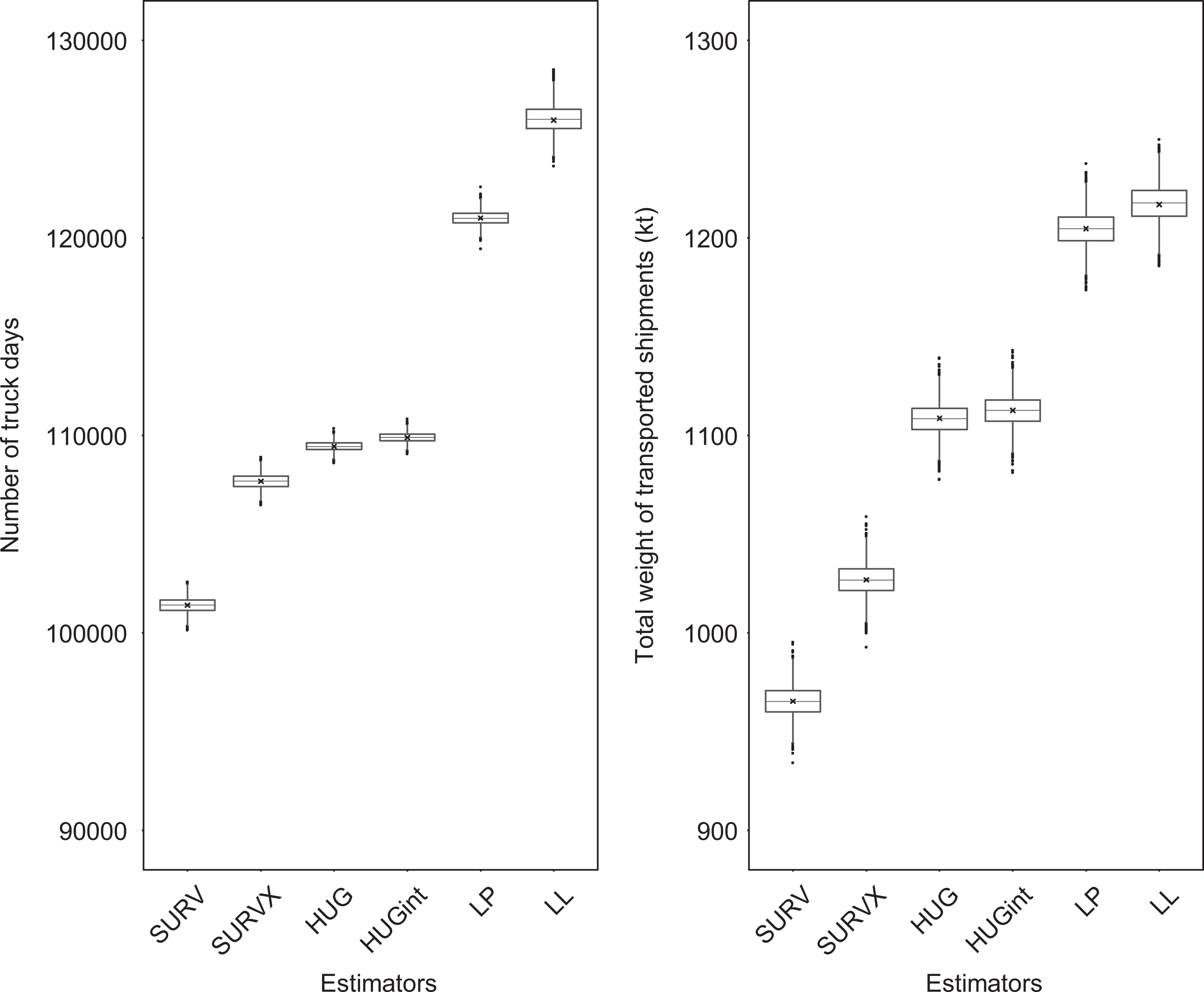
Bootstrap estimates based on 3,000 bootstrap samples of the six estimators for truck days (left panel) and transported shipment weight (right panel). The cross within each box shows the point estimates based on the original data.
Survey and CRC Estimates for Truck Days, Bootstrapped Variance, Standard Error, Confidence Interval, and Amount of Underestimation in the RFTS.
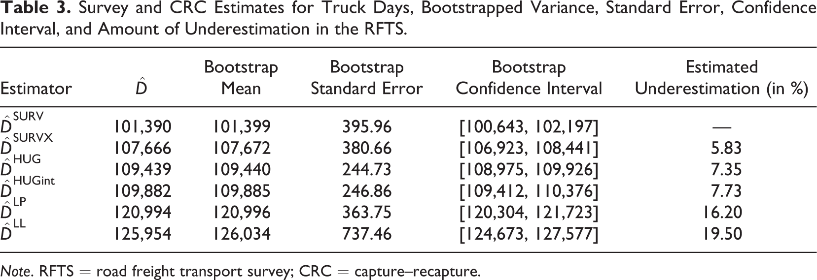
Note. RFTS = road freight transport survey; CRC = capture–recapture.
Survey and CRC estimates for transported shipment weight (in kt), bootstrapped mean, standard error, confidence interval, and amount of underestimation in the RFTS.
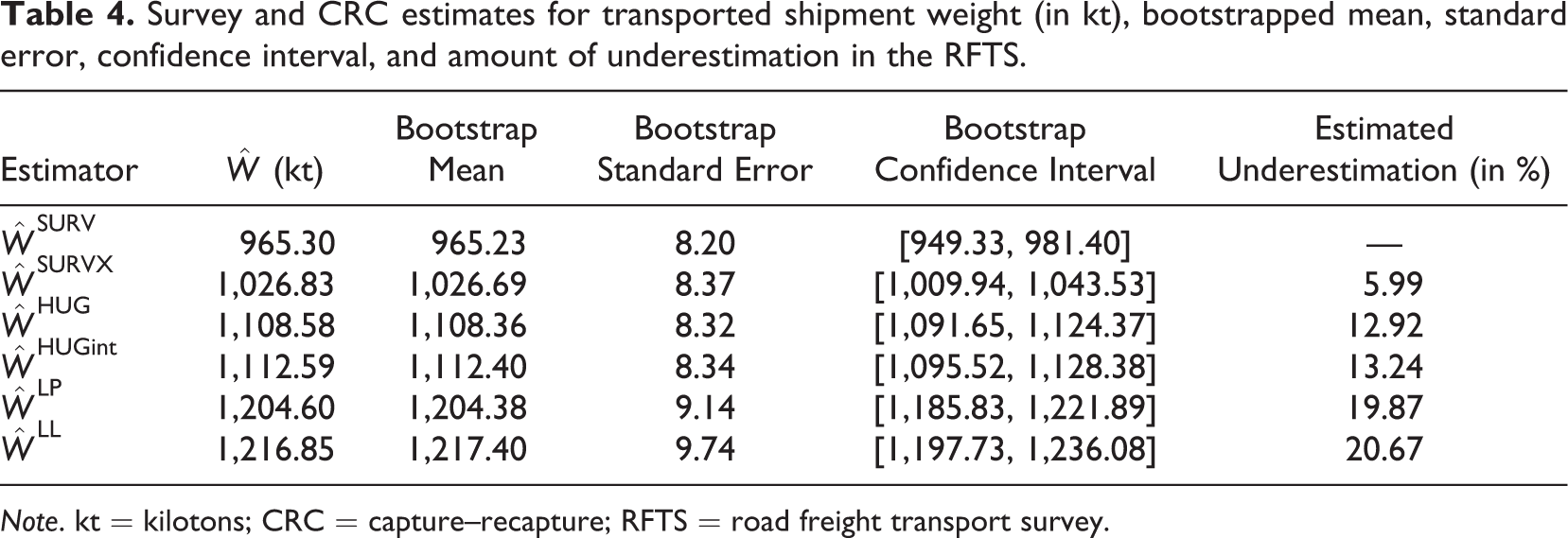
Note. kt = kilotons; CRC = capture–recapture; RFTS = road freight transport survey.
The naive extended survey estimator
The naive extended survey estimator
Bootstrap Diagnostics
The bootstrap estimates shown in Tables 3 and 4 are based on 3,000 bootstrap iterations. Diagnostics showed that the point estimates converge after 1,000 bootstrap iterations. They also showed that the bootstrapped estimates of truck days and transported shipment weight are normally distributed, which indicates that the bootstrapped point estimates are unbiased.
Conclusion
The study presented here is the first application using CRC techniques to correct for misreporting in surveys combining survey, administrative, and sensor data. Six different estimators associated with estimates of number of truck days and the transported shipment weights were applied. We have shown that in relation to the survey estimate, all estimators show large amounts of underestimation in the survey up to 20% for truck days and 21% for the transported shipment weight. Large differences between the applied estimators exist. We recommend relying on the log-linear model for estimating truck days and transported shipment weight. First, it is based on the full likelihood, whereas the logit models are conditional likelihood approaches. Second, it takes heterogeneity in the trucks related to capture and recapture probabilities into account, whereas the Lincoln–Petersen estimator assumes homogeneity.
The CRC method presented here is applicable to any validation study, where survey, administrative, and sensor data (or any other external big data source) can be linked one by one using a unique identifier. We have shown that, by enriching survey data with administrative and sensor data, a bias in the survey estimates can be quantified.
In future studies, we will test stratifications by variables of the administrative databases. Such tests will give insight into potential differences in the percentage of underestimation between, for example, provinces or company sizes. Furthermore, we will implement the Bayesian approach suggested by Huggins (2002), which assumes a beta distribution of the capture probabilities. Finally, we intend to impute the missing data in the administrative databases as proposed by Bakker, van der Heijden, and Gerritse (2017).
Limitations of the study are that the sensor data used are not based on a randomly distributed road sensor network. The stations are located at certain traffic junction points and do not cover rural areas. However, the covariates included in the models should correct for unequal capture probabilities and selection effects by modeling heterogeneity. Therefore, it should be irrelevant where and how many sensors are installed, given the CRC assumptions hold. Furthermore, the WIM software system software does not recognize every single license plate on the front and/or back of the vehicles. If this mechanism is selective, that is, license plates of specific trucks or trailers are not recognized, there might be a selection bias in the trucks recognized. Additionally, the sensors record only one point of time from the entire journey and are not able to capture route characteristics. Hence, there might be deviations from the reported weight of the transported shipment and the weights measured by the road sensors, because shipments might have been unloaded before the truck passing a road sensor station on its journey. To better understand the sources of error for big data, we refer to Biemer (2017).
We consider this study as the first demonstration of methods to use big data in official statistics to estimate bias in survey estimates by combining survey, administrative, and sensor data with CRC techniques.
Footnotes
Authors’ Note
The authors would like to thank the reviewers for their comments and efforts which substantially improved our article. Furthermore, the authors would like to thank Joep Burger for in-depth discussions and thoughtful comments on the article.
Data Availability
To obtain the data used in this research for replication, a secure internet connection (remote access) can be used. The following organizations may be granted access to CBS microdata: Dutch universities, institutes for scientific research, organizations for policy advice or policy analysis, statistical authorities in other European Union countries, and other research institutions authorized to work with the microdata. If your organization does not have authorization to work with the microdata, an application can be made (https://www.cbs.nl/en-gb/our-services/customised-services-microdata/microdata-conducting-your-own-research/applying-for-access-to-microdata). See the official home page for more information (https://www.cbs.nl/en-gb/our-services/customised-services-microdata/microdata-conducting-your-own-research). For more information, please contact microdata@cbs.nl
Declaration of Conflicting Interests
The authors declared no potential conflicts of interest with respect to the research, authorship, and/or publication of this article.
Funding
The authors received no financial support for the research, authorship, and/or publication of this article.
Software Information
The analysis was performed using R (Version 3.2.3). Used R-libraries for data handling are xlsx, data.table, plyr, and reshape2. Modeling was applied using the glm function of R base and the MASS library (as quoted in the text). To plot Figure 1, the libraries rgdal, maptools, and sp were used. To plot ![]() , the libraries ggplot2 and cowplot were used. Complete replication of the analysis is only possible for the organizations mentioned above, if access to CBS microdata is granted. If access is granted, access to the R-scripts to replicate the analysis is made too.
, the libraries ggplot2 and cowplot were used. Complete replication of the analysis is only possible for the organizations mentioned above, if access to CBS microdata is granted. If access is granted, access to the R-scripts to replicate the analysis is made too.