
Abstract
The Rosenthal steady-state analytical solution for the temperature distribution caused by a moving point heat source on a semi-infinite, homogeneous, isotropic solid has been extensively used in modeling metallurgical processes, e.g., arc welding. This study develops a three-dimensional analytical closed-form solution for the temperature field induced by a point heat source moving across a semi-infinite orthotropic solid. The formulation accommodates arbitrary orientations of the heat source’s motion relative to the material’s in-plane principal axes and is extended to solids with finite thickness. Subsequently, using the superposition of the linear solutions, a general methodology is proposed to predict the temperature distribution resulting from an arbitrarily distributed heat source. Verification of the closed-form solution and validation of the distributed heating condition against finite element simulations demonstrate excellent agreement. The analytical framework offers potential for thermal modeling of processing methods used for polymeric composites, e.g., additive manufacturing and continuous welding of thermoplastic composites.
Introduction
With the widespread integration of automation in the industrial processing of various materials and the manufacturing of structural components, the theoretical study of moving heat sources in localized processing has garnered attention since the 1940s with the advent of automated metal welding, and has remained highly relevant with recent advancements in additive manufacturing processes for metallic alloys. Understanding heat propagation within a material subjected to a moving heat source is critical for predicting its thermal history, which directly governs the evolution of microstructural properties and impacts the final product’s quality in terms of mechanical performance and dimensional stability.
Rosenthal
1
developed a foundational theory for thermal analysis of a moving point heat source on isotropic solids. He provided analytical quasi-steady solutions for one-dimensional, two-dimensional, and three-dimensional heat flow in infinite and semi-infinite solids bounded by planes. Meanwhile, Jaeger
2
and Carslaw and Jaeger
3
made seminal contributions in the development of the analytical solutions of the heat conduction equation for different moving source shapes (e.g., band, square, and rectangular with uniform distribution). Later, Hou and Komanduri
4
extended the solutions for additional shapes (e.g., elliptical and circular geometries) and other heat distributions (e.g., parabolic and normal profiles). Despite the advancements, the original Jaeger-Rosenthal closed-form analytical solution for a moving point heat source has remained the well-established framework in the process modelling of joining or additive manufacturing (e.g., beam welding, arc welding, selective laser melting, and laser metal deposition) of isotropic metallic materials (e.g., stainless steel, aluminum alloys, titanium alloys),
5
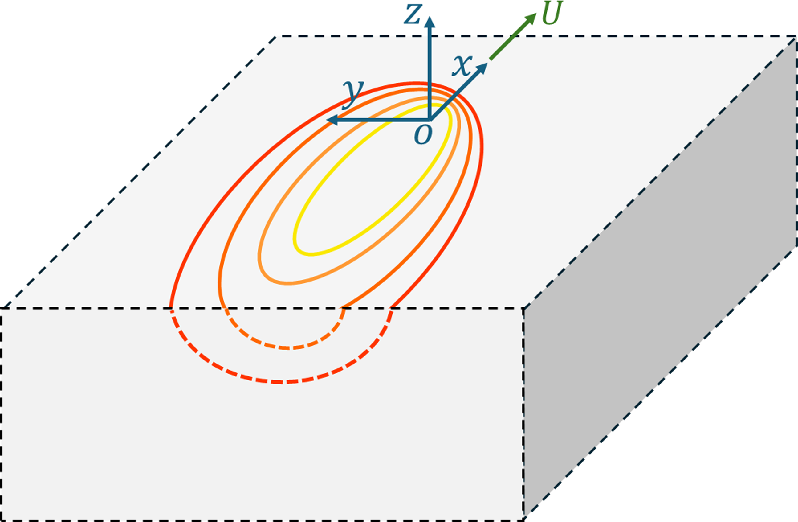
expressing the temperature distribution in a semi-infinite solid as: Representation of the thermal field via moving reference frame attached to a moving point heat source on semi-infinite isotropic solid
5
.

While analytical modeling of a moving heat source on isotropic materials is well-established and no longer considered novel, there remains a need for closed-form analytical solutions for arbitrarily oriented moving heat sources on orthotropic materials, where the thermal conductivity is orientation-dependent. Developing a theoretical framework for orthotropic materials would assist in modeling the thermal processing of fiber-reinforced composites, with examples of polymer-based composites listed in Figure 2. In automated fiber placement (AFP) or automated tape laying (ATL) of thermoset composites (TSCs), typically, an infrared heating system integrated into the placement head increases the temperature of the substrate for enhanced tackiness as the head moves forward during deposition. In AFP of thermoplastic composites (TPCs), where diode laser,
6
hot gas torch,
7
or flash lamp
8
heating systems are typically used to heat the material above its melting point for in-situ consolidation, or for fused filament fabrication (FFF) of fiber reinforced polymers (FRPs) as a similar example, the temperature distribution around the deposition area controls the quality of the final part. A lack of precise prediction over temporal and spatial temperature distribution within the material can lead to violating the process window and causing excessive defects such as material degradation, incomplete healing, and increased void content,
9
which ultimately compromise the mechanical performance of the structure.10,11 Robust and rapid predictive thermal tools allow for online fine-tuning of process parameters, such as the speed, intensity, or distribution of the moving heat source, to achieve the optimal material properties while minimizing energy usage and maximizing efficiency. Application of moving heat source in different processes of polymeric composites.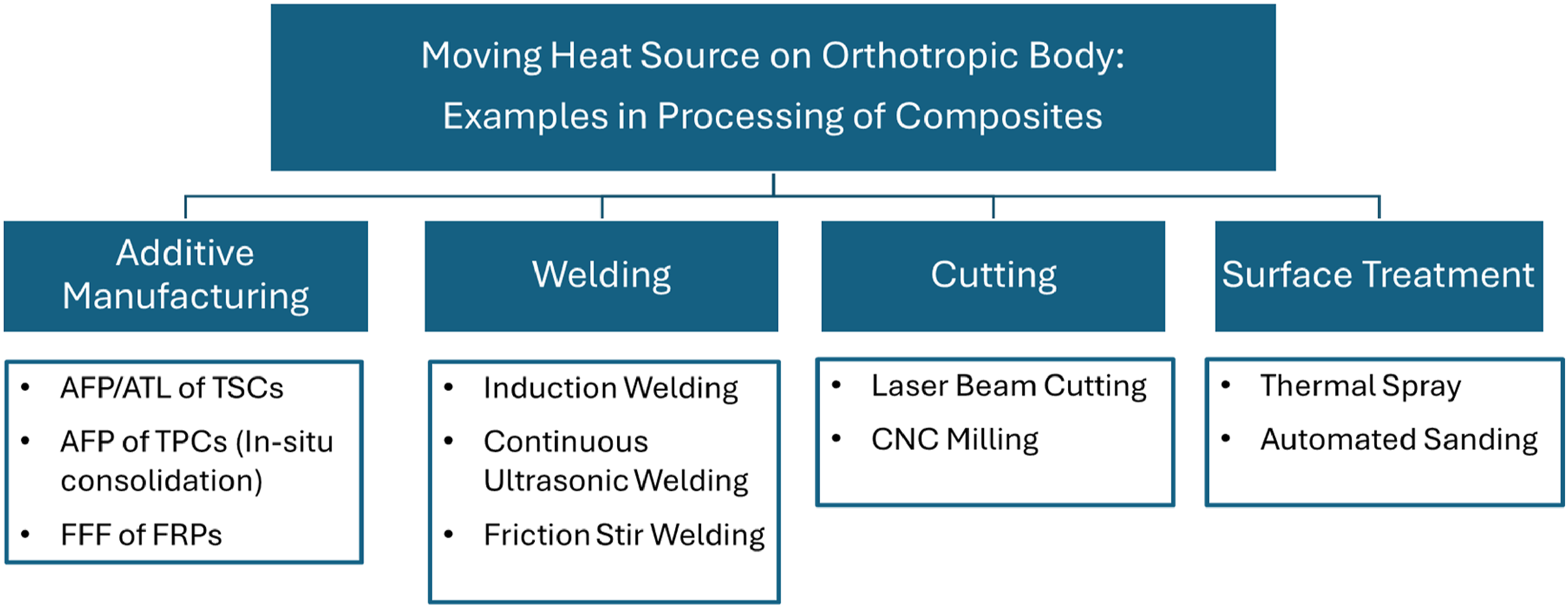
Among the original studies on thermal modeling for in-situ consolidation of thermoplastic composites, Tierney and Gillespie 12 employed a one-dimensional steady-state model to predict the through-thickness temperature distribution when the composite surface is exposed to hot gas impingement. Ghasemi Nejhad et al. 13 developed a two-dimensional analytical model for the thermal analysis of thermoplastic tape laying, modeling a moving uniform heat source over a transversely isotropic domain. Pitchumani et al. 14 also utilized a two-dimensional thermal model to predict the evolution of interfacial bonding, polymer degradation, and void consolidation, with the aim of defining the optimal processing window. While one- and two-dimensional analytical and numerical models continue to be efficient and popular, 15 their accuracy might be limited – for instance, by neglecting heat diffusion across the width. This has motivated the adoption of three-dimensional numerical approaches, especially finite element methods, 16 enabling more accurate thermal predictions, though at the cost of substantially increased computational effort.
The requirement for accurate thermal models is equally critical in continuous in-situ joining techniques for thermoplastic composites (e.g., induction welding, 17 ultrasonic welding, 18 friction stir welding 19 ) where localized melting and solidification of interfacial thermoplastics occurs within the order of a second during the forward motion of the end-effector. On the other hand, in cutting or surface treatment of composites, 20 predicting temperature distribution caused by direct heat source (e.g., laser beam, thermal spray, respectively) or friction-induced heat generation (e.g., CNC milling, automated sanding, respectively) may allow for prevention of thermally softened or minimization of degraded material by optimizing process parameters.
The application of an analytical framework for orthotropic solids can even be extended to additively manufactured isotropic materials if significant porosity, characterized by longitudinal voids/gaps along the deposition axis, renders the homogenized properties effectively orthotropic. Beyond polymers and composites, the framework may be relevant to specific metallic substrates exhibiting orthotropic thermal properties. An example could be single-crystal alloys, such as those used in turbine blades, 21 which display direction-dependent thermal conduction and are subjected to laser-based repair techniques involving localized, moving heat sources.
In this study, an analytical closed-form solution is developed for the temperature distribution induced by a point heat source moving over a semi-infinite orthotropic solid, considering an arbitrary orientation of motion relative to the material’s principal axes. The solution is then extended to accommodate solids with finite thickness. Finally, leveraging the principle of superposition for linear systems, a methodology is proposed to predict the temperature distribution resulting from an arbitrarily distributed heat source. The proposed solutions for the point heat source (in both semi-infinite and finite-thickness cases) and the results for the distributed heat source are validated against finite element simulations, demonstrating excellent agreement.
Theoretical modelling
The following equation represents the three-dimensional heat conduction for an orthotropic solid in Cartesian coordinates:

The spatial coordinates

Consider a point heat source moving horizontally ( Representation of stationary 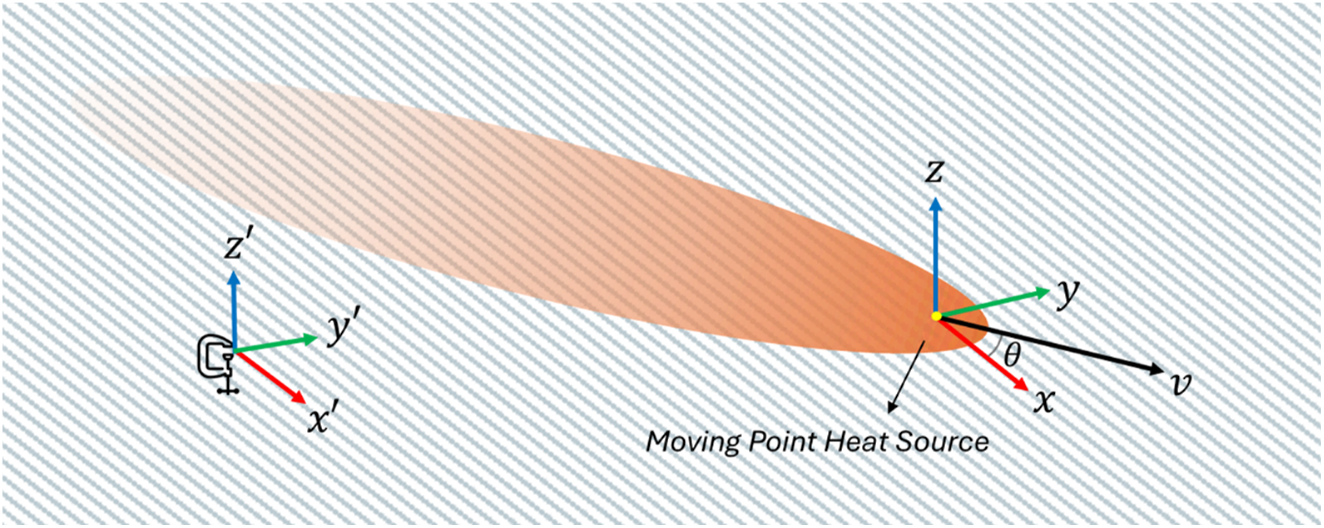
Let


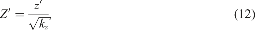
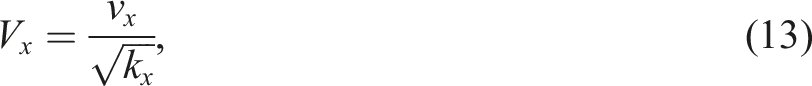
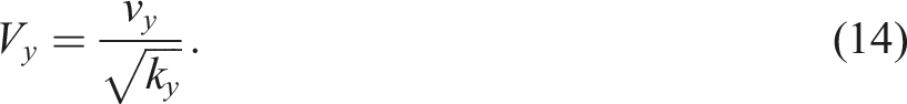
To mathematically simplify the orthotropic nature, spatial coordinates and velocity components can be transformed into scaled variables so that they are normalized based on the corresponding thermal conductivities:


By the transformation of partial derivatives using the chain rule, the quasi-steady heat equation can be expressed in the new coordinates as follows:

Inspired by Rosenthal,
1
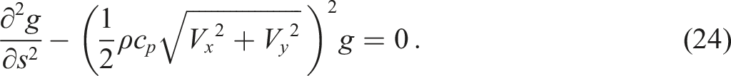
to mathematically separate the effects of advection and symmetric heat diffusion, and to further simplify equation (18), consider:


This equation appears symmetric with respect to the coordinates, and technically,


Since

The solution of this linear second-order homogeneous differential equation is:


Up to this point, the boundary condition at infinity has been applied, leading to
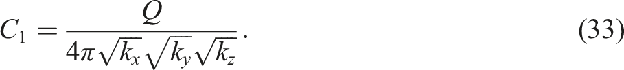
To simplify the determination of the constant

Let us define
Here,
Therefore:

By substituting equations (7), (8), (9), (13), (14), and (21) into equation (34), the temperature distribution in the
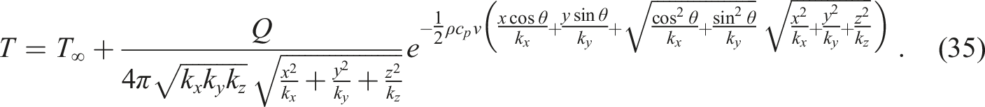
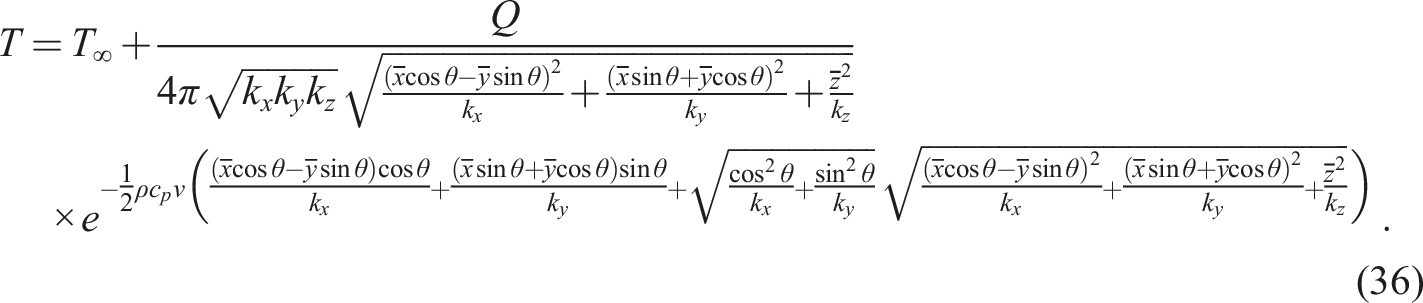
It is often more appropriate to represent the temperature distribution in the
The presented solution provides insight into the temperature distribution within an infinite solid, in which a moving point source with power
The surface centerline (
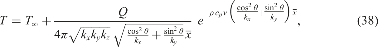

Returning to equation (36), while the developed closed-form solution represents the temperature distribution resulting from a point heat source moving within an infinite orthotropic solid, due to the symmetry of heat propagation with respect to the
Orthotropic Solids with finite Thickness
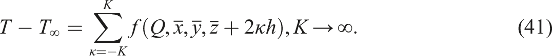
The next step involves evaluating the effect of a moving heat source on solids with finite thickness. For constant and known velocity, material properties, and orientation, as shown in equation (36), the temperature distribution can be represented by the elementary function

As a linear system, the temperature distribution in the solid domain induced by multiple heat sources can be obtained by summation of the effects of all individual sources. Consider an infinite number of point heat sources, spaced Vertically aligned multiple identical point heat sources and corresponding planes of symmetry.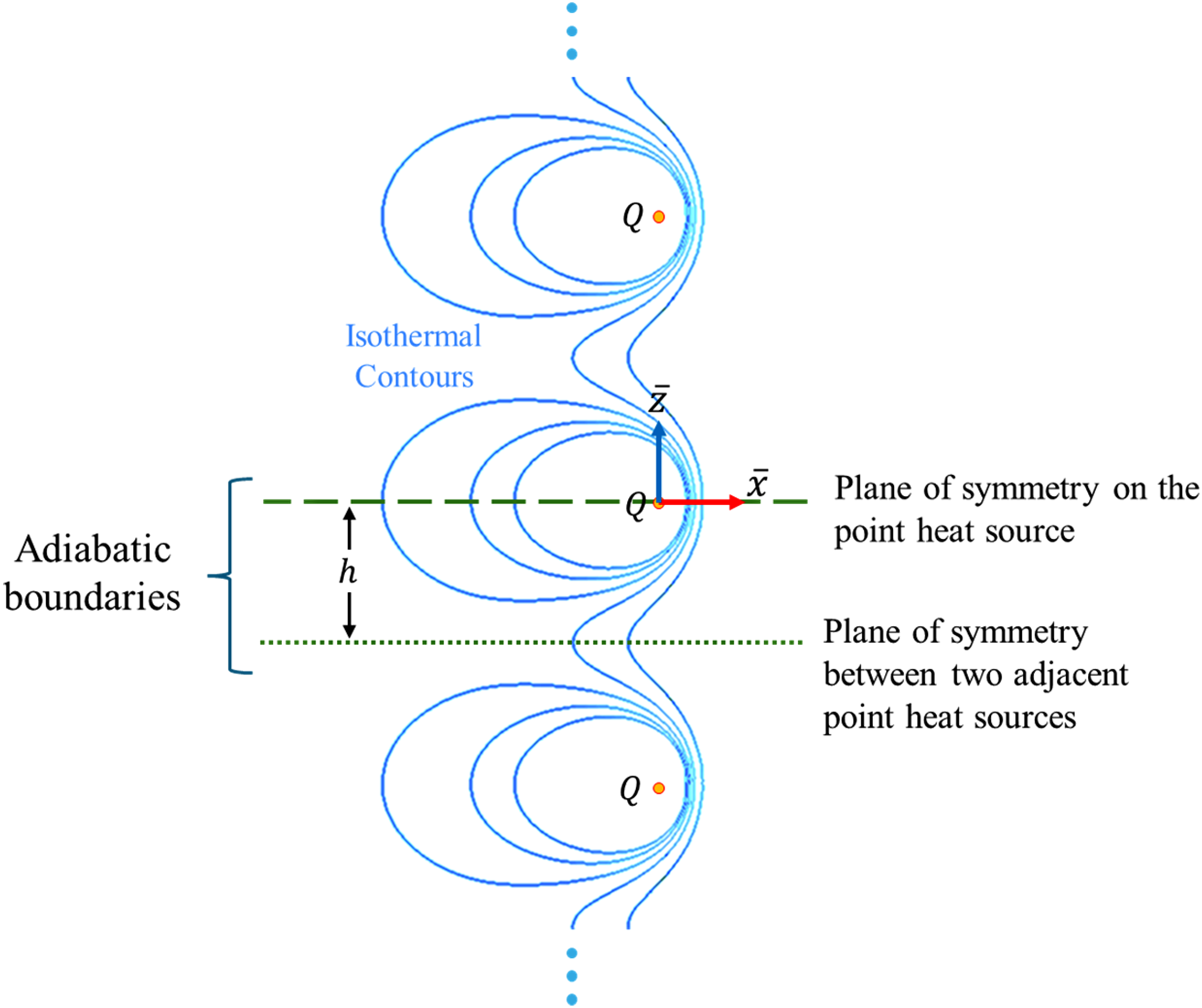
In this configuration, two sets of symmetry planes emerge, functioning as adiabatic boundaries due to the zero heat flux across symmetry planes. The first set consists of horizontal planes passing through the point heat source, one of which is depicted by a dashed line in Figure 4. The second set includes horizontal planes midway between two adjacent heat sources, one of which is shown as a dotted line in Figure 4. The domain
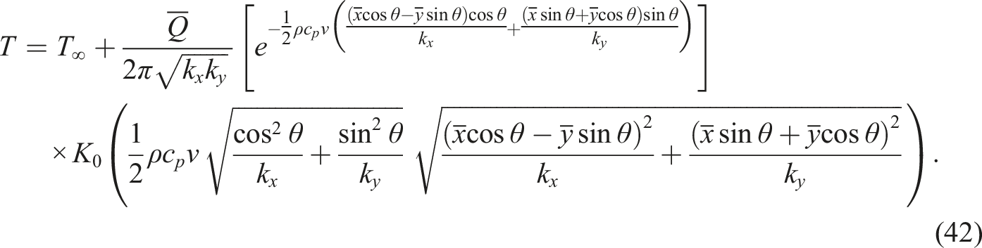
Two-dimensional Solution
Although the primary focus of this study is not on two-dimensional planar heat transfer, such analysis becomes relevant in certain applications – such as thin plates – where through-thickness thermal gradients are insignificant and in-plane heat conduction dominates. An exact two-dimensional solution cannot be obtained as a limiting case of equation (36). Instead, the governing equations should be derived independently, as presented in Appendix C. The final expression for the temperature field is:
Verification
Finite element analysis was performed using COMSOL Multiphysics, employing quadratic Lagrange elements for temperature discretization. In the first step, to perform verification of the analytical model for a semi-infinite solid, the model geometry consisted of a rectangular solid block with dimensions 0.2 m × 0.05 m × 0.01 m. These dimensions were chosen large enough to ensure that the region of interest around the point heat source remained unaffected by boundary effects, thereby satisfying the assumption of a semi-infinite solid. Boundary conditions were specified as follows: constant room temperature was applied to the two lateral faces, the bottom face, and the front (upstream) face, while thermal insulation was imposed on the top face and the back (downstream) face. A point heat source was positioned at the center of the top face (origin) to inject a constant heat power into the system. The relative motion of the heat source was incorporated by defining a translational motion for the solid domain with velocity field of −v in the
The mesh was constructed using tetrahedral elements. Mesh parameters included a maximum element size of 2 × 10⁻³ m, a minimum element size of 1 × 10⁻⁶ m, and a maximum growth rate of 1.05. This meshing strategy resulted in a total of 1,373,879 elements, with the highest mesh resolution concentrated in the vicinity of the point heat source to capture critical thermal gradients, while coarser resolution was employed in regions distant from the area of interest to optimize computational efficiency (see Figure 5 (top)). The input parameters of the simulation are as follows, where the selected material as our example is Carbon-Fiber/Poly-Ether-Ether-Ketone (CF/PEEK) (Table 1): Finite element model in COMSOL Multiphysics. Values of CF/PEEK thermal properties
23
and parameters used for FEM verification.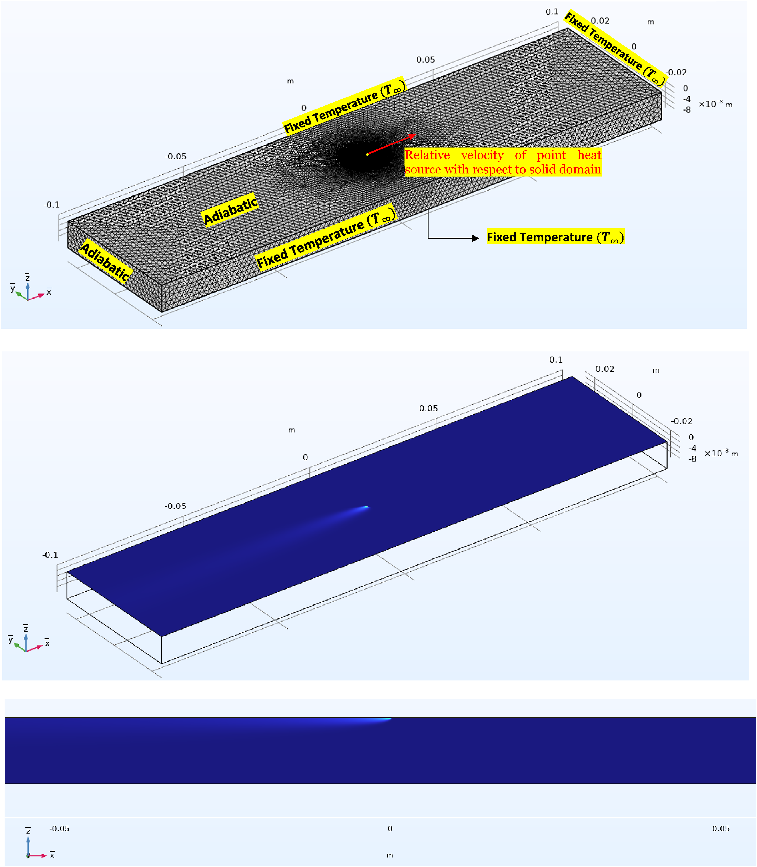
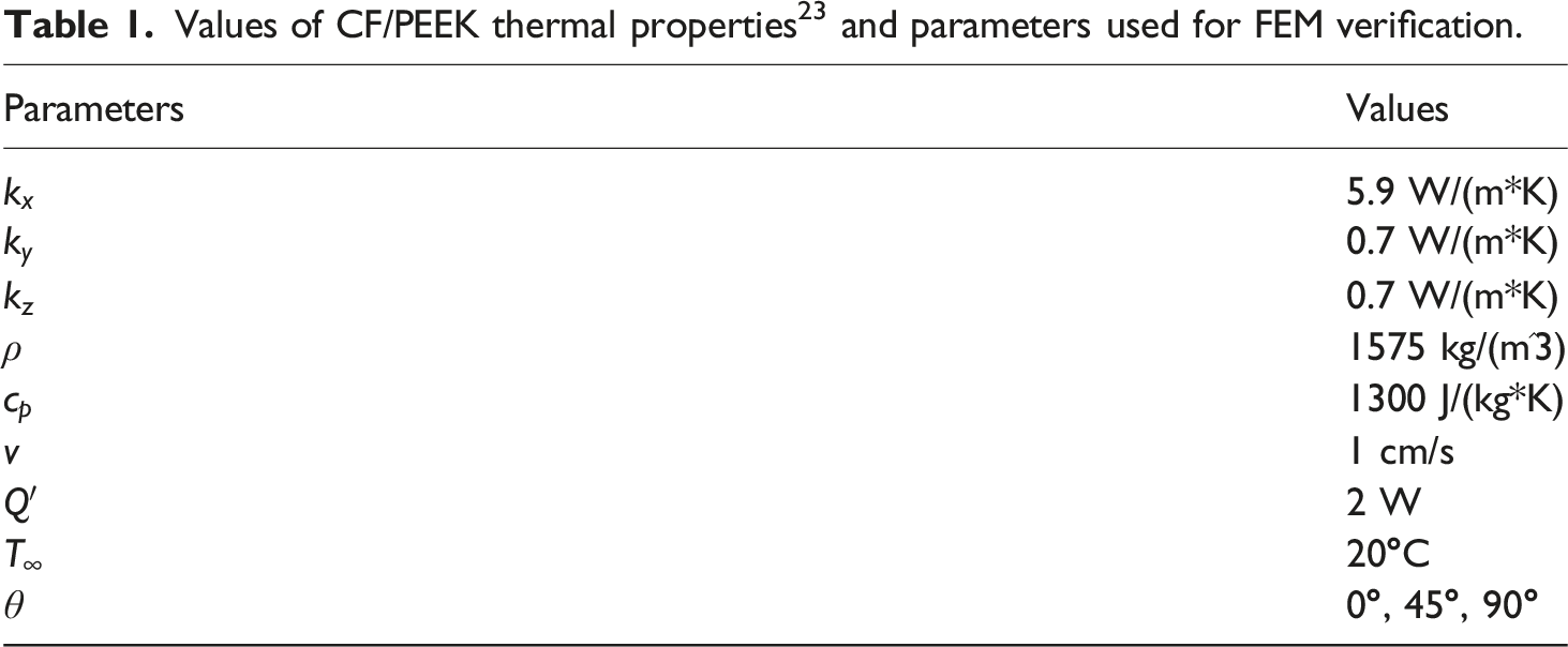
Figure 5 (middle) and (bottom) present color maps of the temperature distribution calculated using the FEM in the
The results of the analytical model for a semi-infinite solid and the finite element analysis are compared in Figure 6, represented as isothermal contours for three different orientations of the velocity vector relative to the material’s principal x-axis. For each orientation, temperature distributions in the (a). Temperature distributions from analytical solution and FEM for a semi-infinite solid with heat source velocity oriented at 0° to the material x-axis: in-plane (top) and through-thickness (bottom). (b). Temperature distributions from analytical solution and FEM for a semi-infinite solid with heat source velocity oriented at 45° to the material x-axis: in-plane (top) and through-thickness (bottom). (c). Temperature distributions from analytical solution and FEM for a semi-infinite solid with heat source velocity oriented at 90° to the material x-axis: in-plane (top) and through-thickness (bottom).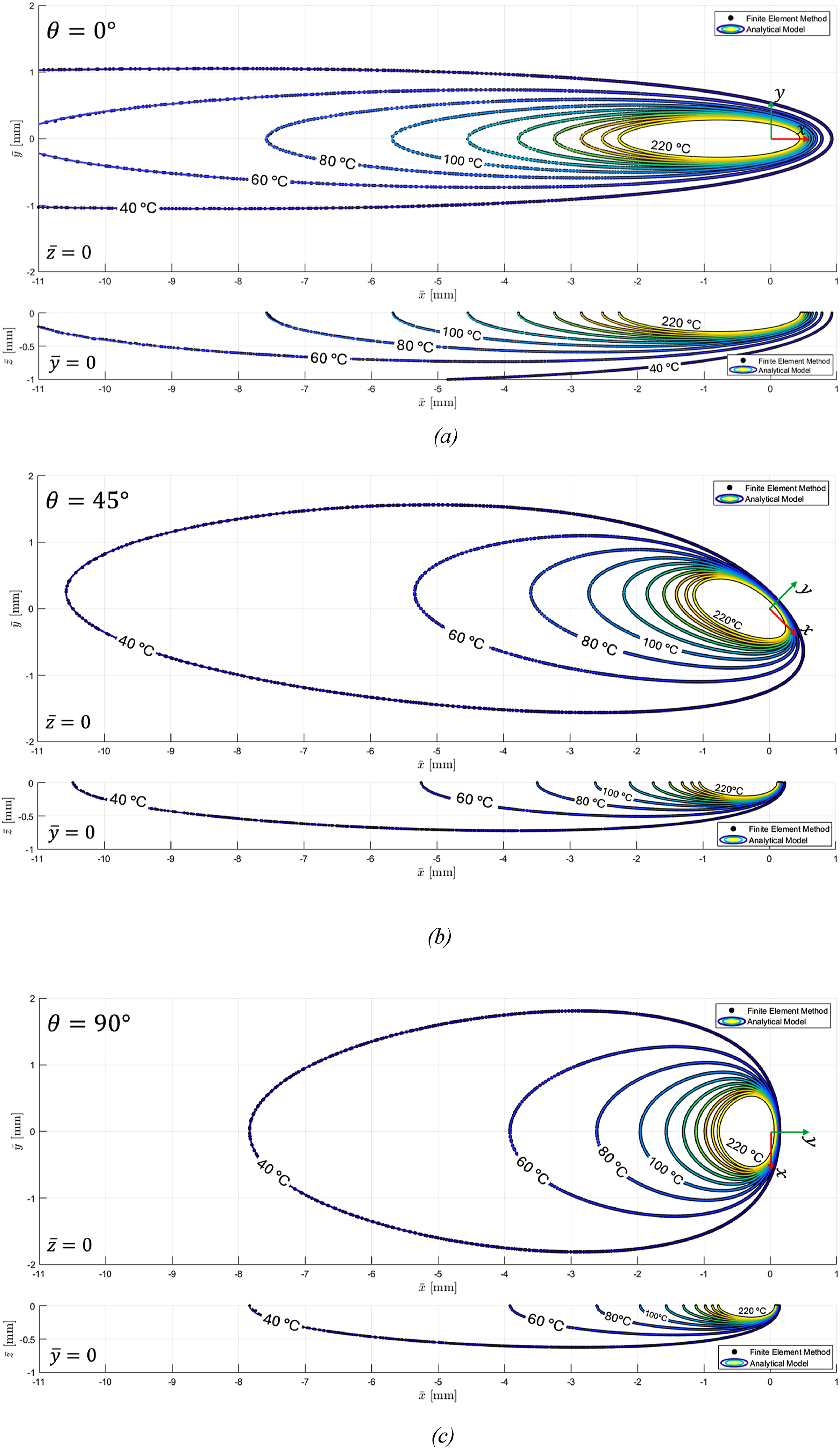
In another stage of verification, the analytical model for a solid with finite thickness (equation (41)) was compared with finite element analysis (FEA). For this case, the geometry of the FEA model was modified by significantly reducing the thickness to 0.25 × 10⁻³ m to account for the influence of the bottom face on the temperature distribution. The boundary condition at the bottom face was then set to adiabatic, while all other parameters, including those listed in Table 1, remained unchanged. The comparison of the analytical and FEA results for the in-plane and through-thickness temperature distributions are illustrated in Figure 7 for three different orientations of the material’s x-axis relative to the heat source velocity. Once again, the excellent agreement between the analytical and FEA results confirms the validity of the analytical framework. In the analytical calculations for this case, the parameter K in equation (41) was set to only 5 (superposition of 11 heat sources), which proved sufficient to achieve high accuracy in the region of interest around the heat source. Due to the exponential decay of the heat source’s effect with distance, selecting a large value for K is unnecessary to maintain acceptable accuracy. (a). Temperature distributions from analytical solution and FEM for a finite-thickness solid with heat source velocity oriented at 0° to the material x-axis: in-plane (top) and through-thickness (bottom). (b). Temperature distributions from analytical solution and FEM for a finite-thickness solid with heat source velocity oriented at 45° to the material x-axis: in-plane (top) and through-thickness (bottom). (c). Temperature distributions from analytical solution and FEM for a finite-thickness solid with heat source velocity oriented at 90° to the material x-axis: in-plane (top) and through-thickness (bottom).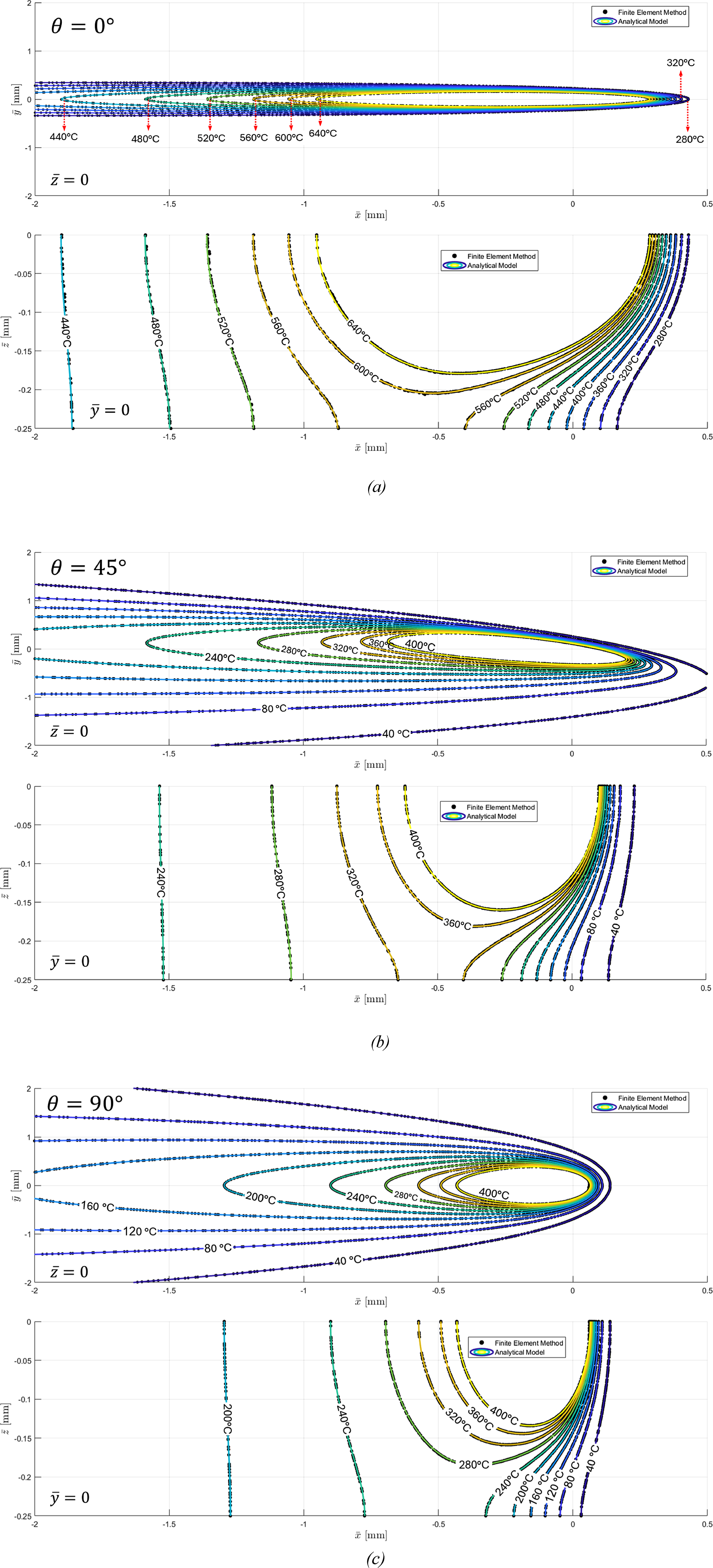
Distributed heat source
The theoretical framework for thermal analysis using a moving point heat source is only valid in practical applications when the heating system delivers highly localized power to the surface. This imposes a limitation on the direct implementation of the existing analytical solution for practical systems. To overcome this constraint, the surface area of the distributed heat flux, which effectively governs the temperature distribution within the solid, is discretized into a series of point heat sources. This discretization aims to replicate the thermal influence of a continuous heat flux distribution. Leveraging the linearity of the thermal system, the temperature at any point within the solid domain can be computed as the superposition of the temperature increments (ΔT) induced by each individual point heat source.
Let Representation of a continuous heat source as an array of discrete point sources.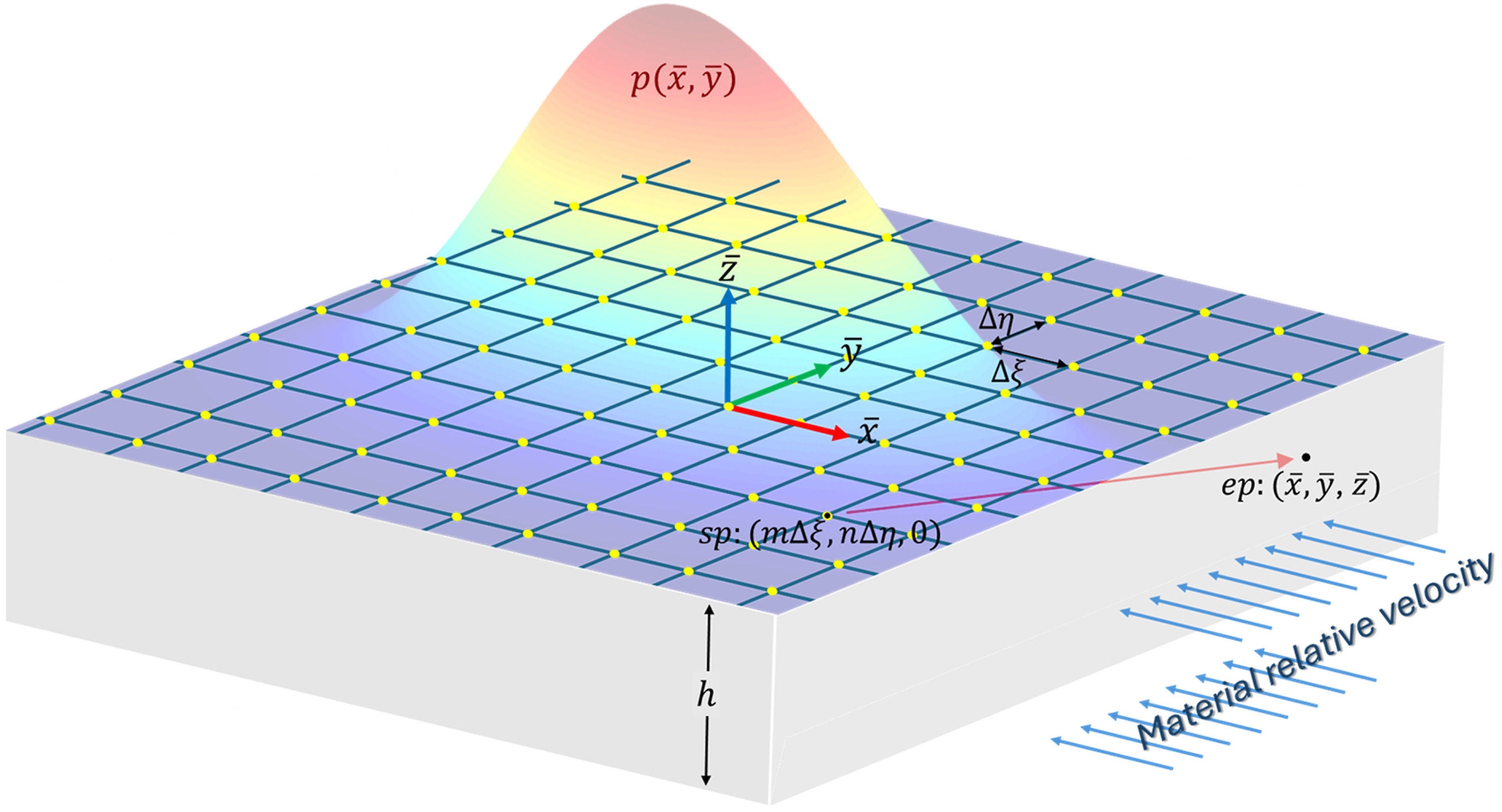
The temperature at an arbitrary excited point (ep) located at 
The bounds of the summation indices,
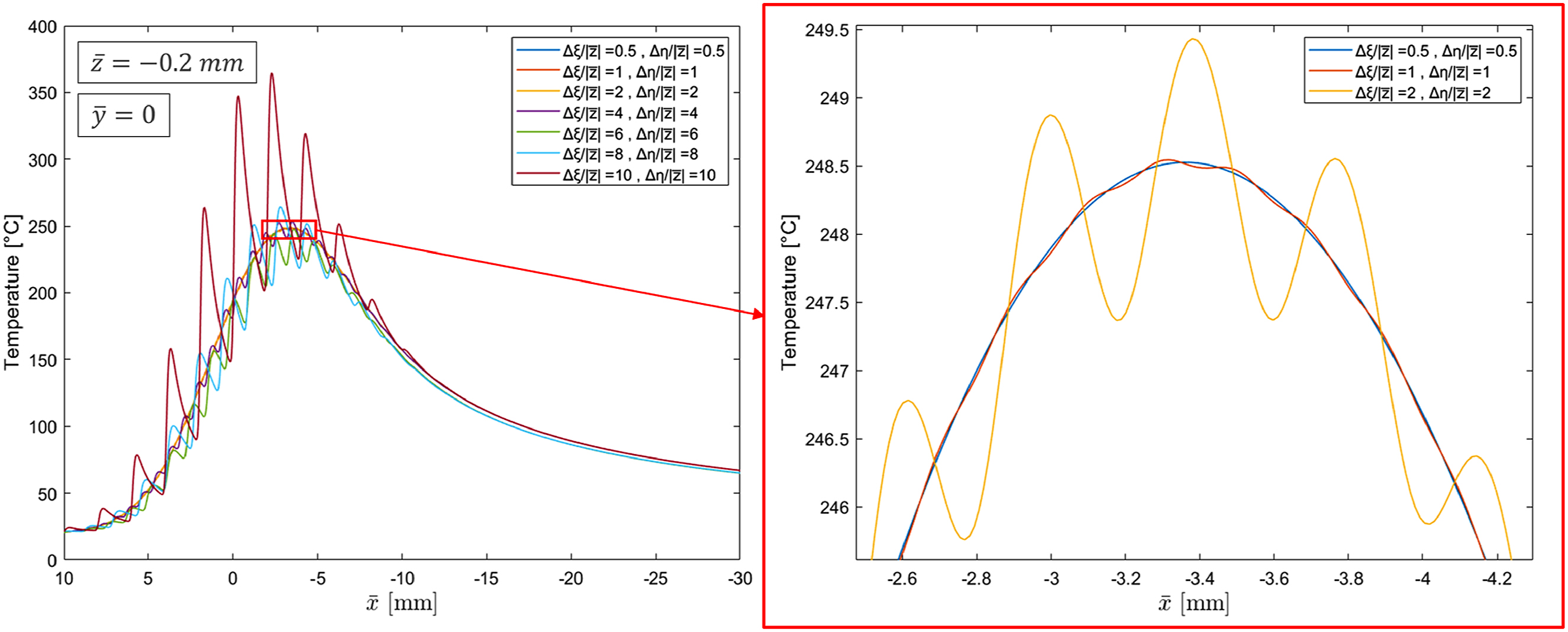
An additional consideration in defining the computational domain is the choice of
Even though the heat flux profile 
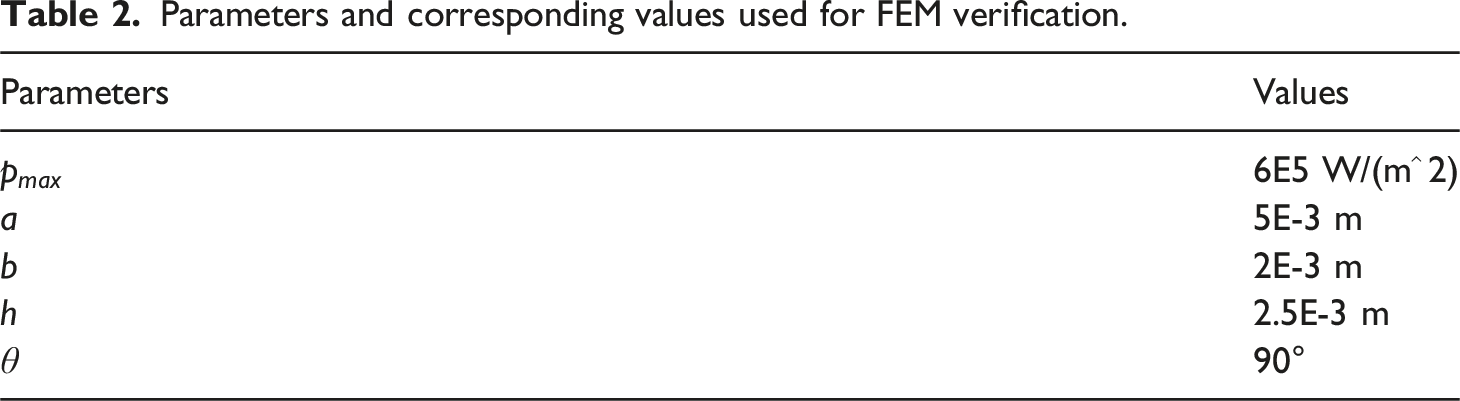
Parameters and corresponding values used for FEM verification.
Calculations were performed at 3000 points within the solid, along a line segment spanning from (10 mm, 0 mm, −0.2 mm) to (−30 mm, 0 mm, −0.2 mm), for various heat source spacings ( Predicted temperature distribution along the axis of motion for different point source spacing ratios.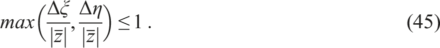
In Figure 10, the temperature distributions predicted by the proposed model are shown at various depths within the Temperature distribution along (left plot) and perpendicular (right plot) to the direction of source motion: Validation of the model for a distributed heat source against FEM results at different depths.
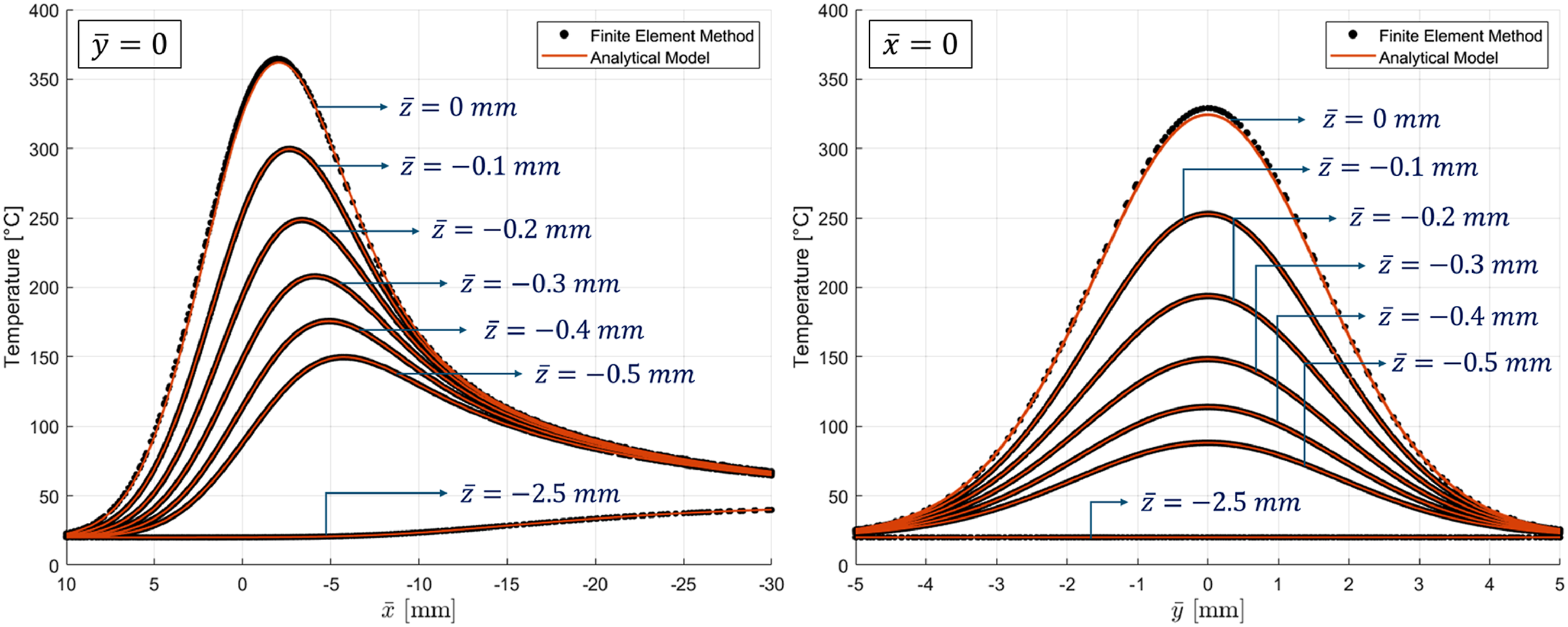
For example, the predicted surface temperature results shown in Figure 10 are obtained by extrapolating the temperature curves at
The steady-state simulation computation time for the COMSOL finite element solver on a typical personal computer was measured at 38 seconds, while the computation time for each point using the analytical model was on the order of centi-seconds (e.g., 0.029 seconds for
A parametric analysis comparing different fiber orientations and heat source velocities under the same distributed heating condition (Table 2) and material properties (Table 1) is presented in Figure 11. The results are visualized using the iso-surface corresponding to the critical glass transition temperature (Tg = 143 Iso-surface of T = 143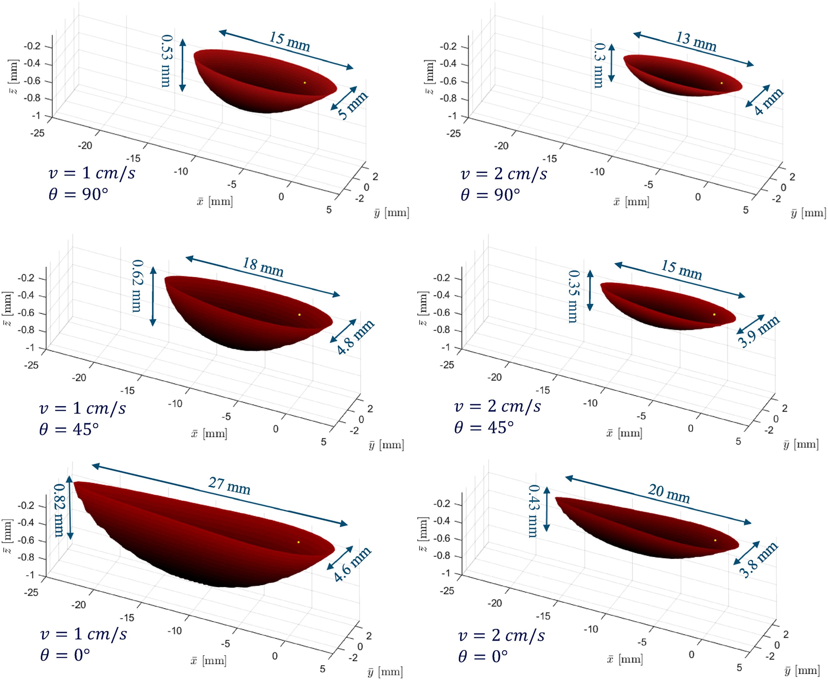
The results indicate that at a velocity of 1 cm/s, reducing the fiber angle from 90° to 0° leads to a moderate reduction (8%) in the width of the region exceeding Tg , while the length of this region increases substantially (80%). A similar trend is observed at 2 cm/s, where the same variation in fiber orientation results in a 5% reduction in width and a 54% increase in length. Regarding the maximum penetration depth of the heated region, decreasing the fiber angle from 90° to 0° results in a 55% increase at 1 cm/s and a 43% increase at 2 cm/s. These findings suggest that as the axis of maximum thermal conductivity (i.e., typically fiber direction for CFRPs) becomes more parallel to the direction of heat source motion, the thermally affected zone becomes not only longer but also deeper. Furthermore, at lower velocities, the dimensions of the heated zone exhibit greater sensitivity to fiber orientation than at higher velocities.
From a different standpoint, increasing the heat source velocity from 1 cm/s to 2 cm/s reduces the size of the region, as the material is exposed to the heat source for a shorter duration. The reduction in length is quantified as 13%, 17%, and 26% for fiber angles of 90°, 45°, and 0°, respectively, while the corresponding reductions in width are 20%, 19%, and 17%. The most pronounced effect is observed in depth reduction, which decreases by 43%, 44%, and 48% for fiber angles of 90°, 45°, and 0°, respectively. Overall, while this analysis highlights the influence of fiber orientation and velocity on the dimensions of the heat-soaked region, the sensitivity of these effects is directly proportional to the material’s degree of orthotropy (e.g.,
Conclusion
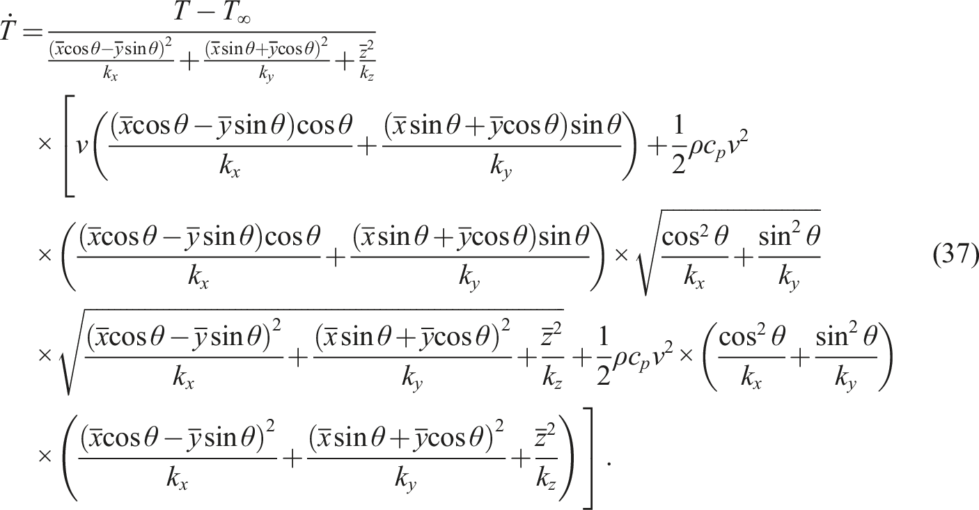
This paper presents a closed-form solution for the thermal analysis of a moving point heat source over a semi-infinite orthotropic solid with arbitrary orientation (e.g., off-axis motion). The resulting temperature distribution is expressed in equation (36), while the local rate of temperature change in the material is formulated in equation (37). While equation (36) was derived for a point heat source of power
Footnotes
Acknowledgements
Financial support from Natural Sciences and Engineering Research Council of Canada is appreciated.
Declaration of conflicting interests
The author(s) declared no potential conflicts of interest with respect to the research, authorship, and/or publication of this article.
Funding
The author(s) disclosed receipt of the following financial support for the research, authorship, and/or publication of this article: Natural Sciences and Engineering Research Council of Canada.