Sage Journals: Discover world-class research

Abstract

Natural fiber-reinforced polymer composites are gaining popularity due to their sustainability and enhanced properties compared to pure polymers. Recently, these composites have been utilized as dielectric materials. In this study, polypropylene (PP) reinforced with maple wood fibers of different lengths (50, 75, and 100 µm) and various fiber concentrations (5%, 10%, 15%, and 20%) were examined. The effects of fiber length and concentration on the dielectric, mechanical, and thermal properties were investigated. All composites exhibited a higher dielectric constant and conductivity than pure PP, along with a lower loss factor. This suggests that adding maple wood fibers generally enhances the dielectric properties. As fiber concentration increases, the dielectric constant tends to rise while the loss factor tends to decrease. TGA results indicated that adding more fibers reduces thermal stability at low temperatures but increases stability at high temperatures. Mechanical testing revealed an increase in strength but a decrease in elongation. However, fiber length did not significantly impact the mechanical properties. SEM analysis showed a uniform distribution of fibers at 5% weight that improves strength, while a 20% weight leads to clustering that weakens the composite.

Keywords

Maple Wood Fiber Composite Dielectric Thermal Analysis Mechanical Properties

Introduction

Polymers are popular materials that have revolutionized numerous industries, thanks to their unique properties and versatility. From consumer goods to advanced engineering applications, polymers offer a range of benefits compared to traditional materials like metals and ceramics.¹ They are generally more affordable to produce, which lowers manufacturing costs and reduces transportation expenses due to their lightweight.² Their soft and flexible properties can help prevent the stiffness of systems, especially in modern applications.³ The ability to mold polymers into complex shapes allows for greater design flexibility, which is particularly beneficial in industries requiring customized components. Furthermore, polymers can be engineered to meet specific performance criteria, including thermal stability, elasticity, and strength. This versatility makes them suitable for a wide range of applications from automotive parts to medical devices.⁴ Despite their numerous advantages, polymers also have notable drawbacks. Many polymers are derived from petroleum, and the disposal of polymer waste has become a significant global concern.⁵ Plastic pollution is a growing issue that threatens the environment and human well-being. These wastes can contaminate soil, waterways, and aquatic ecosystems, and even accumulate in human and animal bodies.⁶ Additionally, some polymers may not match the mechanical strength of metals, necessitating reinforcement for structural applications.

Reinforced polymers are composites that combine a polymer matrix with reinforcing materials.^7,8 These composites enhance the mechanical properties of the base polymer, providing improved strength and durability.^9,10 Fiber-reinforced polymers (FRPs) represent a significant category of reinforced polymers. They consist of a polymer matrix reinforced with fibers made from various materials.¹¹ Glass fiber reinforced polymer (GFRP) is known for its good tensile strength and is widely used in construction and automotive applications.¹² Carbon fiber reinforced polymer (CFRP), on the other hand, is renowned for its high strength-to-weight ratio and finds applications in aerospace and high-performance automotive sectors.¹³ While FRPs enhance mechanical properties, they also come with disadvantages such as higher costs compared to traditional materials and challenges related to sustainability.¹⁴ The choice between natural and synthetic fibers in reinforcement has significant implications for sustainability. Synthetic fibers are often derived from petroleum-based sources, contributing to environmental pollution. Their production processes can be energy-intensive and result in toxic emissions.¹⁵ In contrast, natural fibers are more eco-friendly due to their biodegradability and lower environmental impact during production.¹⁶ They also offer good mechanical properties while being renewable resources.¹⁷ Wood plastic composites (WPCs) are materials made from a combination of wood fibers or wood flour and thermoplastic polymers.¹⁸ Natural wood fibers are plentiful and come from renewable sources. In many cases, they are produced as by-products in the food and furniture industries.^19,20

In the electrotechnical field, polymers play a crucial role as insulators.²¹ Insulators prevent the flow of electric current, ensuring safety and efficiency in electrical systems.²² Dielectrics are materials that act as insulators and have the unique ability to store electrical energy when exposed to an electric field.²³ They possess tightly bonded electrons that hinder the leakage of electric current, resulting in high resistivity ranging from 10⁸ to 10¹⁶ Ω. When a dielectric material is subjected to an electric field, the molecules within the material become polarized.²⁴ This polarization occurs as the positive and negative charges within the molecules shift slightly in response to the external electric field, creating a separation of charge. As a result, the dielectric can store energy in the form of an electric field between its surfaces. This property is crucial in various applications, particularly in capacitors, where dielectrics are used to increase the capacitance by allowing more charge to be stored for a given voltage.²⁵ The effectiveness of a dielectric material is often characterized by its dielectric constant, which quantifies its ability to store electrical energy compared to a vacuum.²⁶ The higher the dielectric constant, the more electrical energy the material can store.

Polymers are increasingly used as dielectric materials due to their excellent insulating properties.²⁷ Commonly used polymers include polyethylene (PE),²⁸ polypropylene (PP)²⁹ polyvinyl chloride (PVC),³⁰ which provide effective insulation for cables and electronic components. Their lightweight nature also contributes to reduced overall system weight in electrical applications. Recent advancements have explored the use of natural fiber-reinforced composites as dielectrics. These materials combine the insulating properties of polymers with the sustainability of natural fibers.³¹ Research indicates that incorporating natural fibers into polymer matrices can enhance dielectric performance while reducing environmental impact.³² In two researches, Khouaja et al^33,34 developed cellulose-based bio-composites to create dielectric materials using thermoplastic matrices, focusing on the dielectric properties of high-density polyethylene (HDPE) and cellulose fiber composites. They concluded that adding cellulose fibers improved the dielectric constant, loss factor, and conductivity of the materials compared to pure polymer. Composites with 50 wt% fiber content exhibited the highest values, while volume resistivity decreased with frequency and fiber content, indicating potential for use as insulators in electrical cables. In another study, Ben Amor et al³⁵ investigated the use of short palm tree lignocellulosic fibers as a reinforcing phase in a polyester matrix to enhance interfacial adhesion. They performed esterification of the lignocellulosic filler using maleic anhydride in an alkaline medium. Dynamic dielectric analysis revealed two relaxation processes in the untreated fiber composite, linked to the glass-rubbery transition and charge carrier diffusion. In contrast, the treated fiber composite exhibited a new relaxation process associated with the molecular motion of amorphous celluloses. George et al³⁶ prepared commingled composites using polypropylene and jute yarns, applying a technique that minimizes shear forces on the natural fibers. They found that as the fiber content increased, the dielectric constant, loss factor, and conductivity improved, while volume resistivity decreased due to enhanced orientational polarization in the jute-reinforced polypropylene composites. However, chemical treatments reduced the hydrophilic nature of jute, leading to lower dielectric properties in treated composites compared to untreated ones. Additionally, dielectric properties increased with temperature up to a certain point before declining, and wet samples exhibited significantly higher dielectric values than dry ones.

It is important to note that fiber length and fiber concentration can significantly affect the mechanical, thermal, and electrical properties of fiber-reinforced composites. However, previous studies on the dielectric properties of natural-fiber-reinforced polymers have not explored these factors. In this study, we investigated the effects of fiber concentration and fiber length on the mechanical, thermal, and dielectric properties of polypropylene reinforced with maple wood fiber.

Materials and methods

Materials

The Hardwood fibers, primarily Maple, were sourced from ARAUCO, a global wood product manufacturer in New Brunswick, Canada. Homopolymer Polypropylene (PP) is supplied by CTMP (Thetford Mines, Quebec). It has a density of 0.9 g/cm³ and a melting temperature of 165°C. Polypropylene-graft-maleic anhydride or MAPP (Aldrich 427845) was used as a coupling agent.

Fiber preparation

After preparing the wood fibers, their moisture content was roughly 65%. To ready them for composite production, we subjected them to drying in a laboratory oven at 70°C until they reached the necessary moisture level of less than 6%.

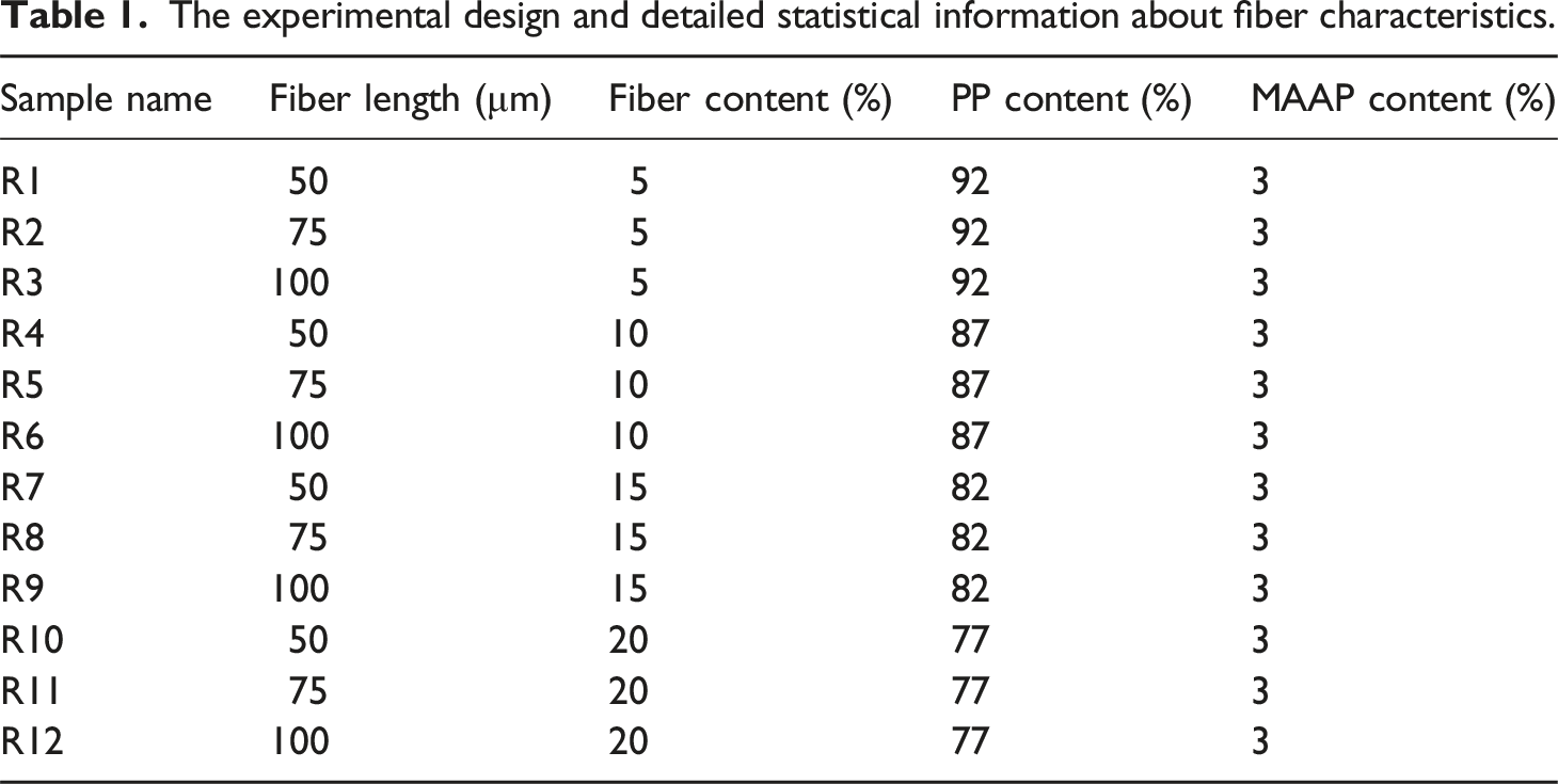
The measured wood fiber lengths exhibited variability. To address this, we categorized them into three lengths: 50, 75, and 100 μm, and then were passed through the mesh (Table 1).

Table 1.

The experimental design and detailed statistical information about fiber characteristics.

Sample name	Fiber length (μm)	Fiber content (%)	PP content (%)	MAAP content (%)
R1	50	5	92	3
R2	75	5	92	3
R3	100	5	92	3
R4	50	10	87	3
R5	75	10	87	3
R6	100	10	87	3
R7	50	15	82	3
R8	75	15	82	3
R9	100	15	82	3
R10	50	20	77	3
R11	75	20	77	3
R12	100	20	77	3

The distribution process adhered to the ASTM standard, utilizing mesh sizes of 53, 75, and 106 μm through the use of standard testing sieves. Fibers that passed through the 106 μm mesh but not the 75 μm mesh were classified as “long,” while those that passed through the 75 μm mesh but not the 53 μm mesh received the label “medium.” Fibers that passed through the 53 μm mesh were designated as “short.” Furthermore, the aspect ratio (the ratio of fiber length to width) of all the fibers was determined and presented in Table 2. To further reduce the moisture content to less than 6%, all the fibers underwent additional drying in a laboratory oven at 70°C for a duration of 24 hours.

Table 2.

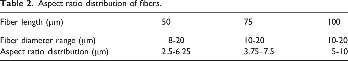
Aspect ratio distribution of fibers.

Fiber length (μm)	50	75	100
Fiber diameter range (μm)	8-20	10-20	10-20
Aspect ratio distribution (μm)	2.5-6.25	3.75–7.5	5-10

Maleic anhydride grafted polypropylene (MAAP) for all reinforced samples was maintained constant at 3%.

Composite preparation

Each sample’s components, which included PP, MAPP, and Maple fibers, were pre-mixed to create uniform compounds. Following the preparation of PP, MAPP, and fibers, and preceding the material blending step within the extruder. All the raw materials underwent thermal analysis using DSC and TGA instruments. This analysis was conducted to determine the optimal temperature required for the formulation of material combinations essential for composite fabrication. Subsequently, these compounds were blended within a twin-screw extruder “torque” rheometer (mixer) (THERMO HAAKE) operating at a screw speed of 50 rpm and a temperature of 180°C. The resulting mixture was then extracted from the mixing bowl and transformed into pellets using a knife grinder (RESTCH). These pellets underwent a drying process at 105°C for a duration of 24 hours before thermocompression.

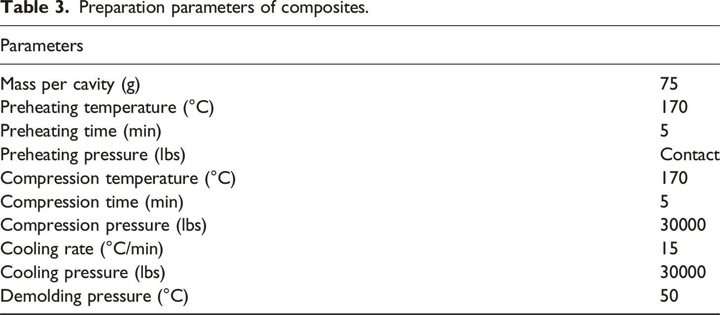
Finally, the pellets were subjected to thermocompression molding using a Carver 30 Ton Compression Press in accordance with the guidelines (ASTM) outlined in Table 3.

Table 3.

Preparation parameters of composites.

Parameters
Mass per cavity (g)	75
Preheating temperature (°C)	170
Preheating time (min)	5
Preheating pressure (lbs)	Contact
Compression temperature (°C)	170
Compression time (min)	5
Compression pressure (lbs)	30000
Cooling rate (°C/min)	15
Cooling pressure (lbs)	30000
Demolding pressure (°C)	50

Characterization

Different tests were conducted on PP/ wood composites to explore how fiber length and content affect their thermal, mechanical, and dielectric properties, as well as their morphology. The investigations focused on understanding the relationships between these factors and the overall performance of the composites.

Thermal characterization

The thermal, melting, and crystallization characteristics of the samples were analyzed using Differential Scanning Calorimetry (DSC) with a DSC-Q20 calorimeter from TA Instruments (New Castle, DE, USA). The analysis was performed across a temperature range of 0°C to 250°C, including a complete heating and cooling cycle at a rate of 10°C/min under a nitrogen flow of 50 mL/min. Samples weighing between 10 and 15 mg were placed in aluminum pans for measurement.

Thermogravimetric analysis

To assess the thermal stability and degradation behavior of the composites, a thermogravimetric analyzer (TGA) (Model: Q50, TA Instruments, New Castle, DE, USA) was utilized. The analysis covered a temperature range from 25°C to 561°C. Samples weighing between 10 and 15 mg were heated from 30°C to 600°C at a rate of 30°C/min in a nitrogen atmosphere with a flow rate of 40 mL/min.

Tensile test

The mechanical properties were thoroughly examined using tensile and three-point bending tests for both the raw material (PP) and the composites. Each sample underwent five repetitions of the tests. The tensile test was conducted at room temperature with a displacement rate of 5 mm/min, following the ASTM-D638 standard using a Zwick universal testing machine (Zwick, Type: 8406, USA).

Three-point bending test

The mechanical performance of the maple wood fiber/ PP composites was evaluated using a three-point bending test, following ASTM D790 standards. Specimens were prepared in rectangular shapes, measuring 100 mm in length, 10 mm in width, and 3 mm in thickness. The tests were conducted using a Zwick universal testing machine with a crosshead speed set at 2 mm/min to ensure controlled loading conditions. The span length between the supports was maintained at 80 mm to facilitate accurate measurement of flexural strength and modulus. During the test, the load was applied at the midpoint of the specimen until failure occurred, allowing for the recording of load-displacement curves.

Morphology Investigation

Scanning electron microscopy (SEM) was employed to investigate the microstructural characteristics and fiber dispersion of the maple wood fiber/ PP composites. Prior to imaging, composite samples were freeze-fractured. To enhance conductivity and minimize charging effects during imaging, the samples were coated with a thin layer of gold using a sputter coater. The prepared samples were mounted on aluminum stubs with conductive carbon tape and placed in the SEM chamber. Imaging was conducted using a Hitachi SEM (TM4000Plus II, Japan).

Dielectric spectroscopy

The dielectric properties were measured using a Broadband Dielectric Spectrometer (BDS) from Novocontrol Technologies, Germany. The setup included an Agilent E4991 impedance analyzer operating over a frequency range from 1 MHz to 3 GHz. Small cylindrical samples of the wood/PP composite, measuring 10 mm in diameter and 3 mm in thickness, were placed between two parallel electrodes made of gold. This configuration facilitated efficient dielectric measurements. By selecting two fixed frequencies (2.45 GHz and 915 MHz) this study aimed to provide a comparative analysis of dielectric behavior of composites with different fiber lengths and concentrations. A sinusoidal voltage was applied to generate an alternating electric field. The resulting current was measured, allowing for the calculation of phase shifts and subsequent determination of dielectric properties. To ensure statistical significance and reliability, measurements were taken in three replicates for each frequency. The dielectric spectroscopy assessed several key parameters, including the dielectric constant (ε′), which reflects the material’s ability to store electrical energy; dielectric loss (ε′′), indicating energy dissipation within the material; and electrical conductivity (σ), measuring the material’s ability to conduct electric current. These parameters are crucial for understanding how the composite behaves under electrical fields.

Results and discussion

Thermal properties

Effect of fiber length

To investigate the thermal behavior of polypropylene/wood (PP/Wood) composites and the effects of fiber concentration and fiber length on their thermal properties, Differential Scanning Calorimetry (DSC) was conducted on the prepared composites. The results of the DSC curves for samples R1, R2, and R3 are presented in Figure 1 to examine the influence of fiber length in constant fiber concentration (5%) on the thermal behavior of the composites.

Figure 1.

Effect of fiber length on DSC curves.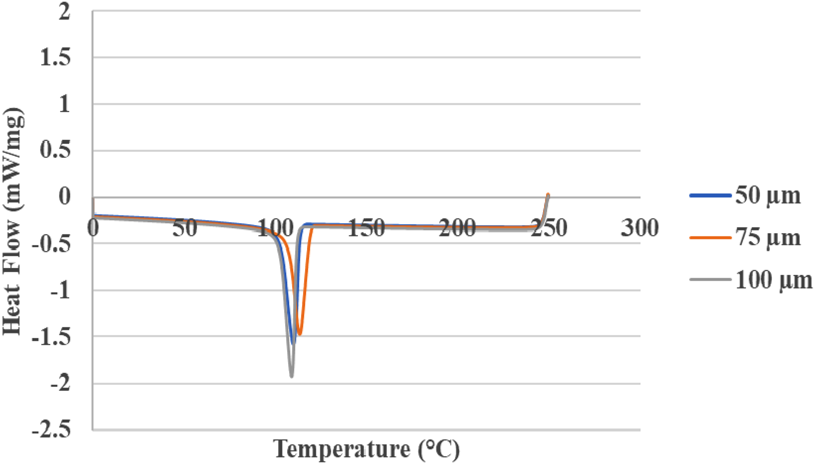

All three curves exhibit a similar pattern, indicating comparable thermal behavior across different fiber lengths. Each curve shows a significant exothermic peak around 100°C–120°C, which corresponds to the crystallization temperature (Tc) of the polypropylene matrix. The deepest peak, reaching approximately −2 mW/mg, is associated with the 100 μm fibers. This deep peak suggests a strong exothermic reaction, likely indicating a pronounced crystallization or thermal transition related to the 100 μm fibers. This implies that the longer fibers restrict the molecular mobility of the PP matrix and delay their arrangement, allowing for greater energy release before transitioning to a different state.

The intermediate peak depth, around −1.6 mW/mg, is associated with the 50 μm fibers, while the shallowest peak, approximately −1.5 mW/mg, corresponds to the 75 μm fibers. These two peaks indicate a moderate exothermic reaction, suggesting that the thermal properties of this composite are influenced by fiber length but not as significantly as in the case of the 100 μm fibers. The crystallization process begins around 120°C for all samples and completes at about 100°C, with slight variations among them. Chollakup et al³⁷ investigated the effects of fiber length and fiber content on the characteristics of pineapple leaf fiber-reinforced thermoplastic composites. They found that adding fiber at different lengths did not result in significant differences in the melting temperatures of pure PP and their composites.

The sample with 75 μm fibers shows a slightly broader crystalline range, possibly indicating a more gradual crystallization process. Additionally, this sample exhibits a crystallization point that is 4°C higher. This was previously observed for melting process by Zhang et al,³⁸ who studied the effect of fiber length and dispersion on the properties of long glass fiber-reinforced thermoplastic composites based on poly (butylene terephthalate) (PBT). They found that the melting point of the LGF/PBT composites initially increases and then slightly decreases as the original lengths of the glass fibers increase. This behavior is attributed to the glass fibers in the composites hindering the molecular motions of the matrix resins and enhancing the rigidity of the LGF/PBT composites.

Before and after the crystallization peak, all curves display relatively stable baselines. No significant exothermic peaks are observed, suggesting the absence of other thermal events within the measured temperature range. The similar overall thermal behavior across different fiber lengths indicates that fiber length does not drastically alter the thermal properties of the polypropylene matrix. However, the slight variations in peak depth and width suggest that fiber length does have a subtle influence on the crystallization characteristics of the composite. This phenomenon is demonstrated by Li et al,³⁹ who studied the effect of fiber length on the mechanical and thermal properties of glass fiber-reinforced polyphenylene sulfide composites. They found that fiber length distribution had minimal influence on the thermal stability of the composites.

Effect of fiber concentration

The results of the DSC curves for samples R1, R4, R7 and R10 are presented in Figure 2 to examine the influence of fiber concentration with constant length (50 μm) on the thermal behavior of the PP/Wood composites.

Figure 2.

Effect of fiber concentration on DSC curves.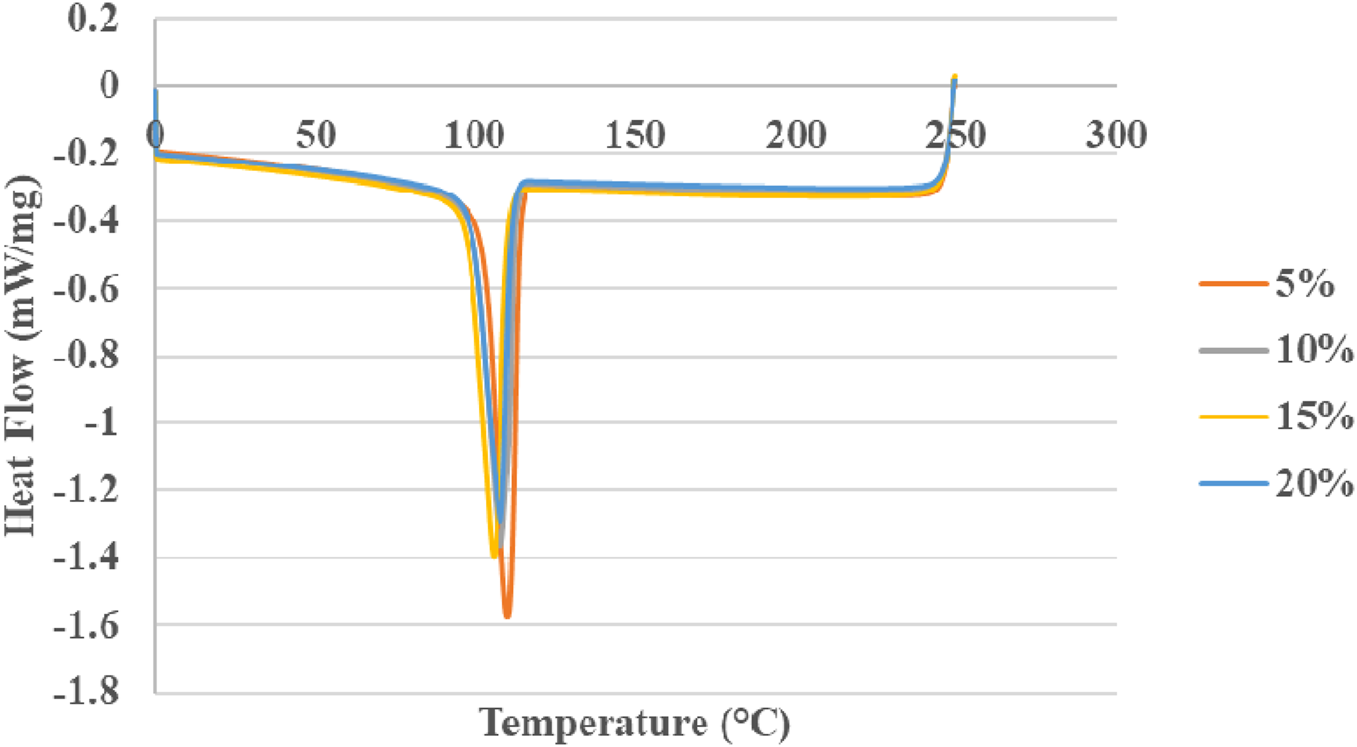

All four curves follow a similar overall pattern, indicating comparable thermal behavior across different fiber concentrations. Each curve exhibits a prominent exothermic peak around 95°C–115°C. The thermal analysis reveals that the 5% fiber concentration exhibits the deepest peak, reaching approximately −1.6 mW/mg, while the 10% and 15% fiber concentrations show slightly shallower peaks at around −1.4 mW/mg. In contrast, the 20% fiber concentration presents nearly identical peaks, reaching about −1.3 mW/mg. As fiber concentration increases, the depth of the exothermic peak decreases. The effect seems to plateau between 10% and 15% fiber content, as these curves are nearly identical.

No other clear peak is observed during cooling. All samples appear thermally stable up to about 250°C. The peak of the curves occurs at the same temperature for all samples, indicating that the fiber concentration does not significantly affect the crystallization temperature (Tc). The similar overall thermal behavior across different fiber concentrations indicates that fiber content does not drastically alter the thermal properties of the PP matrix. However, the decrease in peak depth with increasing fiber content suggests that wood fibers influence the crystallization characteristics and potentially the crystallinity of the PP matrix. The slight differences in baseline slopes before after crystallization indicate that fiber concentration affects the heat capacity of the composites.

Thermogravimetric analysis

Thermogravimetric analysis (TGA) was conducted on pure polypropylene (PP), pure maple fibers, and composite samples over a temperature range of 23 to 600°C. This analysis is essential for understanding how the addition of fibers, their concentration, and length affect the thermal degradation of the samples. Specifically, the TGA results can be presented in terms of two main factors: The impact of fiber length and fiber concentration on thermal stability and the degradation process.

Effect of fiber length

To investigate the effect of fiber length on the thermal stability and degradation of polypropylene/wood composites, TGA curves for pure PP and composite samples R1, R2, and R3 are illustrated in Figure 3. This analysis allows for a detailed examination of how varying fiber lengths in constant fiber concentration (5%) influence the thermal behavior of the composites, providing insights into their degradation patterns under heat exposure.

Figure 3.

Effect of fiber length on TGA curves.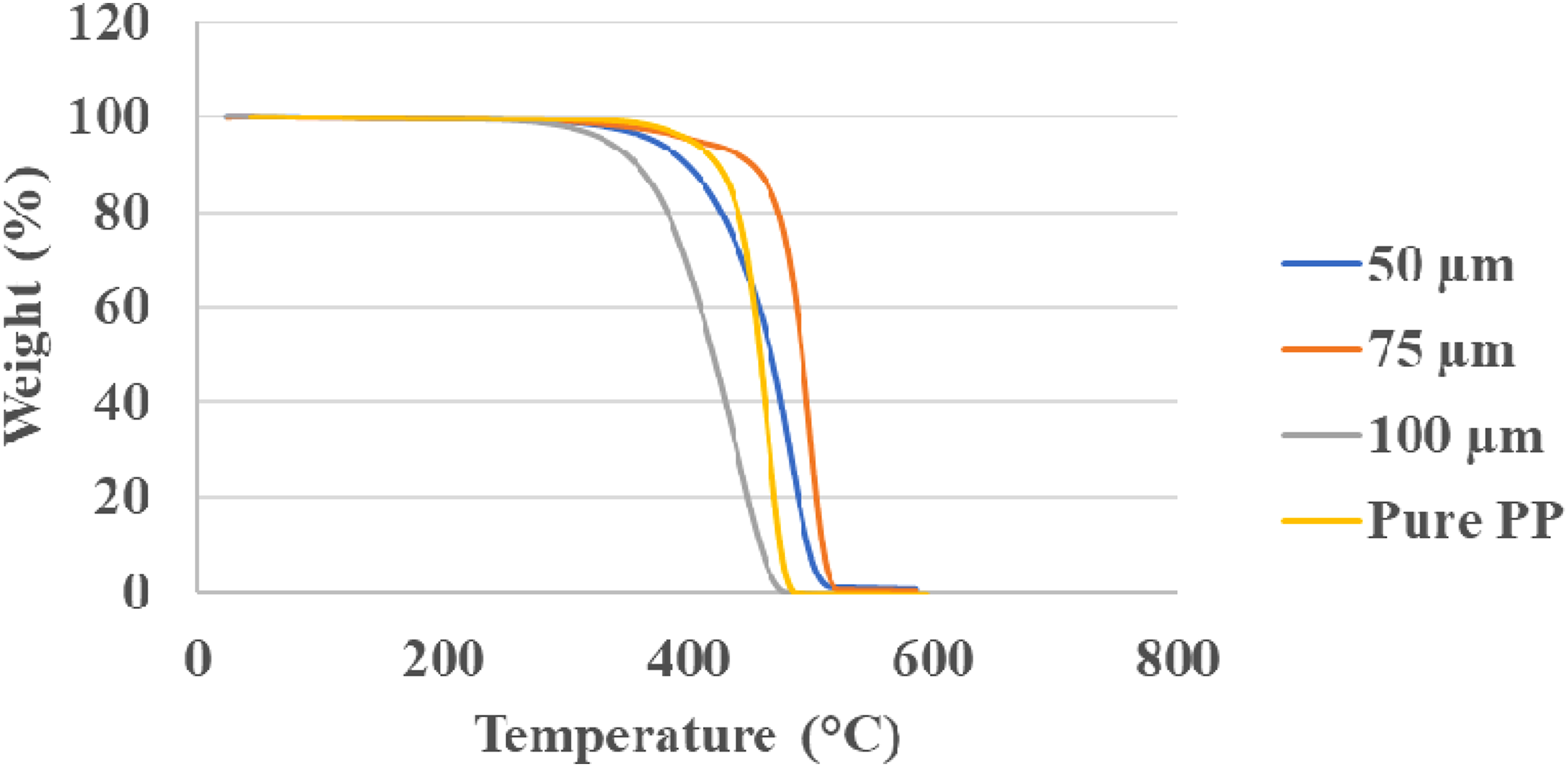

As shown in Figure 3, all samples remain thermally stable up to 270°C, with no signs of degradation detected. The addition of fibers can significantly alter the thermal behavior of the composites, affecting the initial degradation temperature (IDT), final degradation temperature (FDT), and residual weight after degradation. The sample containing 100 µm fibers exhibited the earliest onset of thermal degradation, with a 2% weight loss occurring at 298°C. In contrast, weight loss for samples with 50 µm and 75 µm fibers occurred at 330°C and 345°C, respectively, while pure PP experienced weight loss at 371°C. These results indicate that incorporating fibers into the PP matrix reduces its IDT and thermal stability at lower temperatures. Among the composite samples, the one with 75 µm fibers demonstrated the best IDT, while the sample with 100 µm fibers exhibited the poorest thermal stability.

Regarding final degradation temperature, the sample with 100 µm fibers had the lowest FDT at 484°C, followed by pure PP at 489°C, then the sample with 50 µm fibers at 519°C, and finally the sample with 75 µm fibers at 525°C. This suggests that pure PP degrades faster than the composites and that fiber addition allows the composites to withstand higher temperatures than pure PP. Additionally, shorter fibers showed greater thermal stability.

In terms of residual weight percentage after degradation, results indicate that pure PP and the sample with 100 µm fibers completely degraded. However, the sample with 75 µm fibers retained 0.5% of its weight, while the sample with 50 µm fibers retained 1%. This indicates that the length of the fiber does not have a significant impact on the residual weight. Nurazzi et al⁴⁰ discuss why natural fiber/polymer composite samples exhibit lower thermal stability at lower temperatures while being more stable at higher temperatures. They present thermogravimetric (TG) and derivative thermogravimetric (DTG) curves for oil palm shell powder in the range of 35 to 900°C. The analysis indicates that natural fibers typically degrade in three main stages, with significant thermal decomposition occurring between 215 and 470°C. The initial stage involves weight loss attributed to moisture evaporation.⁴¹ In the second stage, the thermal degradation of the primary lignocellulosic components begins, while the third stage involves the decomposition of cellulose, characterized by a shoulder peak corresponding to hemicellulose and a tail peak indicating the end of lignin decomposition. The residual weight observed in this final stage is likely due to char or other byproducts from decomposition reactions. Hemicellulose decomposes at a maximum temperature of 290°C with an activation energy of up to 150 kJ/mol, whereas lignin decomposes between 280°C and 520°C, requiring up to 229 kJ/mol for activation energy.⁴²

Effect of fiber concentration

To examine the effect of fiber concentration on the thermal stability and degradation of polypropylene/wood composites, thermogravimetric analysis (TGA) curves for pure PP, pure maple fiber, and composite samples R1, R4, R7, and R10 (each with a constant fiber length of 50 µm) are presented in Figure 4. This analysis provides insights into how varying fiber concentration influences the thermal behavior and degradation characteristics of the composites.

Figure 4.

Effect of fiber concentration on TGA curves.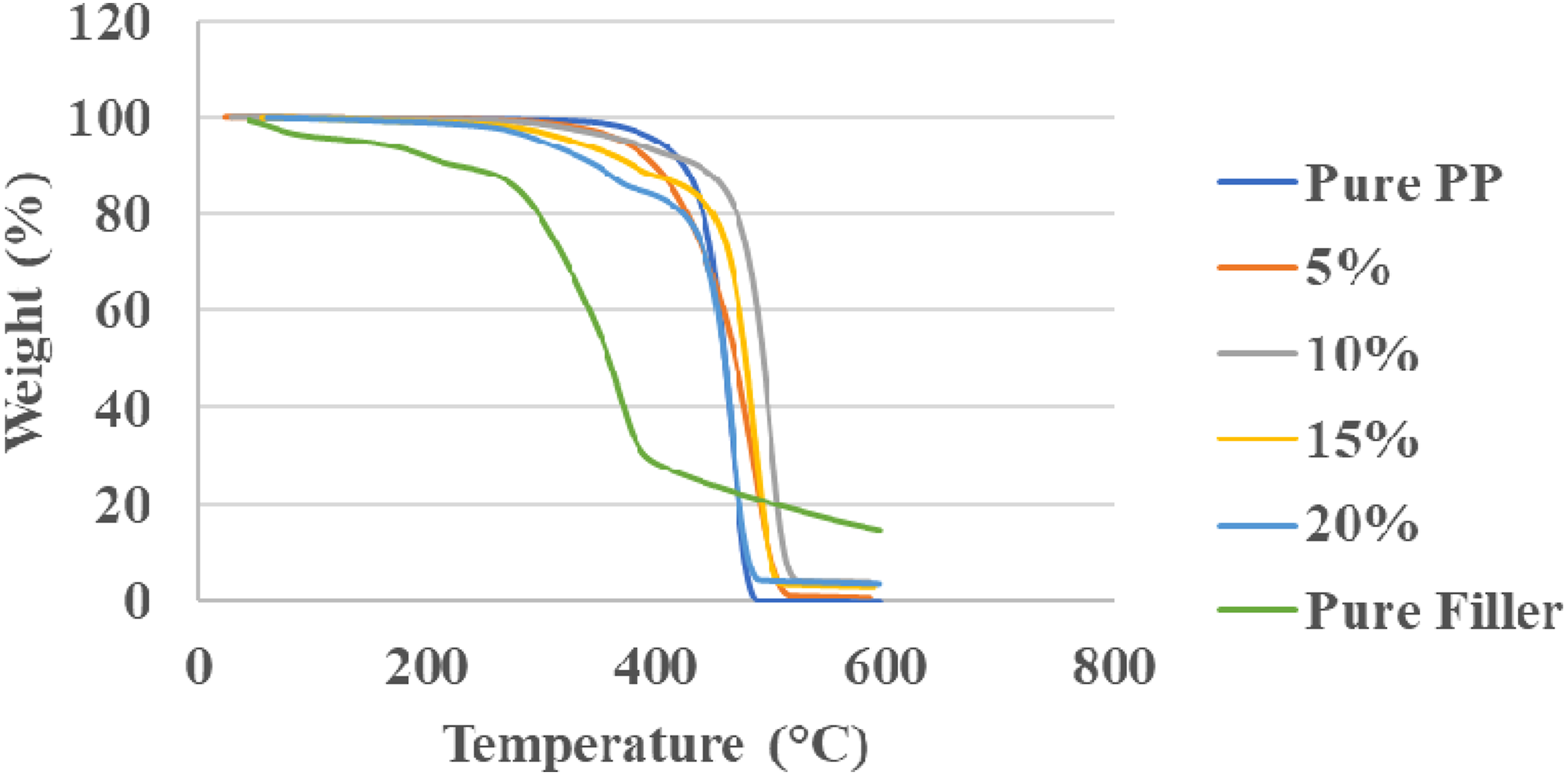

As illustrated in Figure 4, the degradation behavior of pure maple samples is distinctly different from that of pure PP. The degradation of maple fibers begins immediately when the test starts, while PP degradation initiates at 371°C. As previously mentioned, this initial stage of fiber degradation can be attributed to the evaporation of water within the fibers. However, the maple sample experiences a slower degradation rate compared to pure PP, resulting in a remaining weight of 15% after degradation, whereas pure PP degrades completely. This difference due to the varying degradation mechanisms between neat PP and natural fibers. The degradation of natural fibers follows a two-stage process: a low-temperature stage associated with the degradation of hemicellulose and a high-temperature stage linked to the degradation of lignin.⁴³ It is evident that as the fiber content increases in composite samples, their degradation behavior more closely resembles that of the fibers. Notably, the sample with 5% fiber content resembles PP more than those with higher fiber content. Consequently, composites containing fibers exhibit lower thermal stability at lower temperatures than pure PP, as they begin to degrade earlier. These findings agree with previous findings.^44,45 The findings in this study are also consistent with another study by Ghanbar et al⁴⁶ on the thermal stability of PP/bagasse composite foams, which obtained same TGA results for virgin PP, virgin bagasse fiber, and composites with 25% and 50% bagasse loading in the PP matrix. In a study on high-density polyethylene (HDPE) reinforced with various types of natural fibers, including pine, bagasse, rice straw, and rice husk, Liu et al⁴⁴ concluded that all natural fiber-reinforced HDPE composites demonstrate lower thermal stability compared to neat HDPE. Similarly, in another study on PVC, Xu et al⁴⁵ examined the effects of different fiber types (bagasse, rice straw, rice husk, and pine fiber) on composite properties and found that incorporating natural fibers reduced the thermal stability of PVC/natural fiber composites compared to neat PVC. In contrast, fiber-reinforced composites exhibit greater stability at higher temperatures. Their final degradation temperature is elevated, resulting in a greater remaining weight at the end of the process. This behavior improves with increasing fiber content; for instance, a sample with 20% fiber content retains the most weight after degradation, with 4.3% remaining weight among all tested composites.

Mechanical properties

Figure 5 shows the stress-strain diagrams under tensile loading for polypropylene composites reinforced with maple wood fiber. This study includes three fiber lengths of 50, 75, and 100 μm in constant reinforcement content, as well as four weight percentages of 5%, 10%, 15%, and 20% of the reinforcement content. In Figure 5(a), the effect of the fiber length is investigated, there is no great difference in the elastic area and mechanical properties at the UTS point. Table 4 has been prepared for a more detailed and quantitative examination of the mechanical results (three parameters of tensile strength, Young’s modulus and uniform elongation) for all composites. According to Table 4, three composites reinforced with wood fiber with lengths of 50, 75 and 100 μm have ultimate tensile strength of 26.46, 27.13 and 25.20 MPa, respectively. These results show the low effect of fiber length on tensile strength. For these three composites, Young’s modulus and elongation are close to each other, although composites with fiber lengths of 75 and 100 μm have the highest and lowest properties, respectively. Yuan et al⁴⁷ study on the effect of wood fiber length on the mechanical properties of PP reinforced with maple wood fiber at a fiber content of 50% showed that the tensile strength and tensile modulus were very similar across different fiber lengths. However, they concluded that longer fibers led to lower mechanical properties because increasing the length of the wood fiber made it more difficult for polymer molecules to fully penetrate the vessels of the wood fiber.

Figure 5.

Stress-strain diagrams for polypropylene composites reinforced with maple wood fiber under tensile loading: (a) investigation of fiber length and (b) effect of weight percentage of reinforcement.

Table 4.

Quantitative results extracted from tensile and three-point bending tests.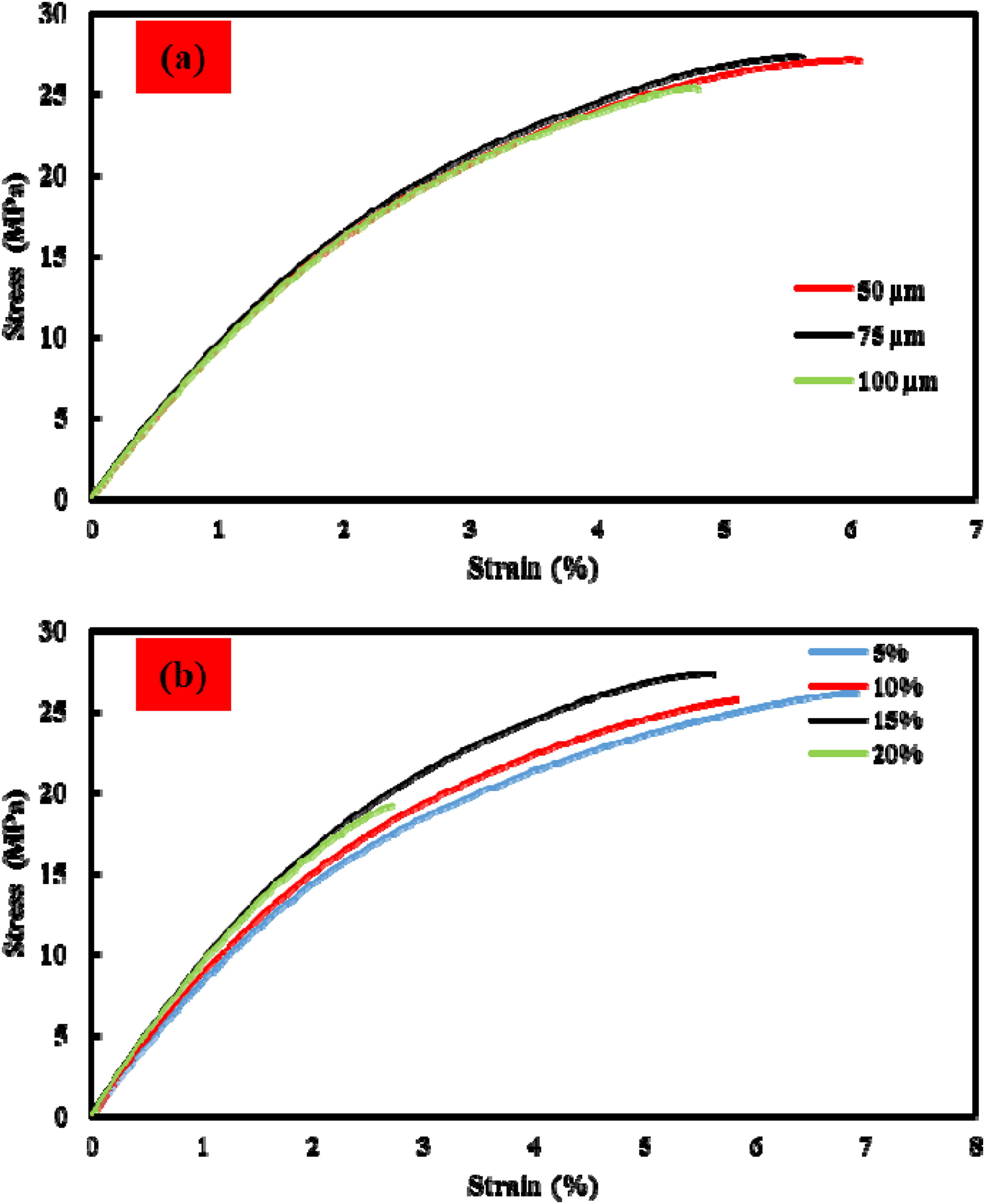

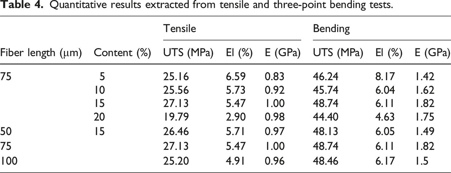
Fiber length (μm)	Content (%)	Tensile			Bending
Fiber length (μm)	Content (%)	UTS (MPa)	El (%)	E (GPa)	UTS (MPa)	El (%)	E (GPa)
75	5	25.16	6.59	0.83	46.24	8.17	1.42
	10	25.56	5.73	0.92	45.74	6.04	1.62
	15	27.13	5.47	1.00	48.74	6.11	1.82
	20	19.79	2.90	0.98	44.40	4.63	1.75
50	15	26.46	5.71	0.97	48.13	6.05	1.49
75		27.13	5.47	1.00	48.74	6.11	1.82
100		25.20	4.91	0.96	48.46	6.17	1.5

Figure 5(b) shows the effect of reinforcing content by fabricating a composite containing four percentages of 5%, 10%, 15% and 20%. According to the stress-strain diagrams, with the increase of the weight percentage of the content from 5 to 15%, the Young’s modulus and tensile strength increase and the elongation decreases. This trend shows the strengthening role of fibers. When the fiber content reaches from 15% to 20%, the mechanical properties decrease drastically and the tensile strength, elongation and Young’s modulus decrease. Based on the quantitative data in Table 4, the highest tensile strength for the sample containing 15% by weight of wood fiber has a tensile strength of 27.13 MPa. Of course, the composite containing 5% also has the highest elongation at 6.59%. As expected, increasing the reinforcement content can increase the strength until it has a uniform and homogeneous distribution, and its increase from a higher optimal value not only cannot have a reinforcing role, but can also be associated with a decrease in strength. The decrease in the strength of the composite containing 20% can also be justified by this reason. By increasing the weight percentage of the content from 15% to 20%, the tensile strength drops from 27.13 MPa to 19.89 MPa.

In Figure 6, the effect of fiber length and reinforcement content under three-point bending loading has been investigated. Similar to the results of mechanical properties under tensile loading, the composites prepared with variable fiber length have almost the same mechanical behavior, although the composite with 75 µm fiber length has a slight advantage. Also, the rate of change in tensile loading is higher than in bending. The tensile strength for composites prepared in three fiber lengths of 50, 75, and 100 µm is 48.13, 48.74, and 48.46 MPa, respectively.

Figure 6.

Stress-strain diagrams for polypropylene composites reinforced with maple wood fiber under three-point bending loading: (a) investigation of fiber length and (b) effect of weight percentage of reinforcement.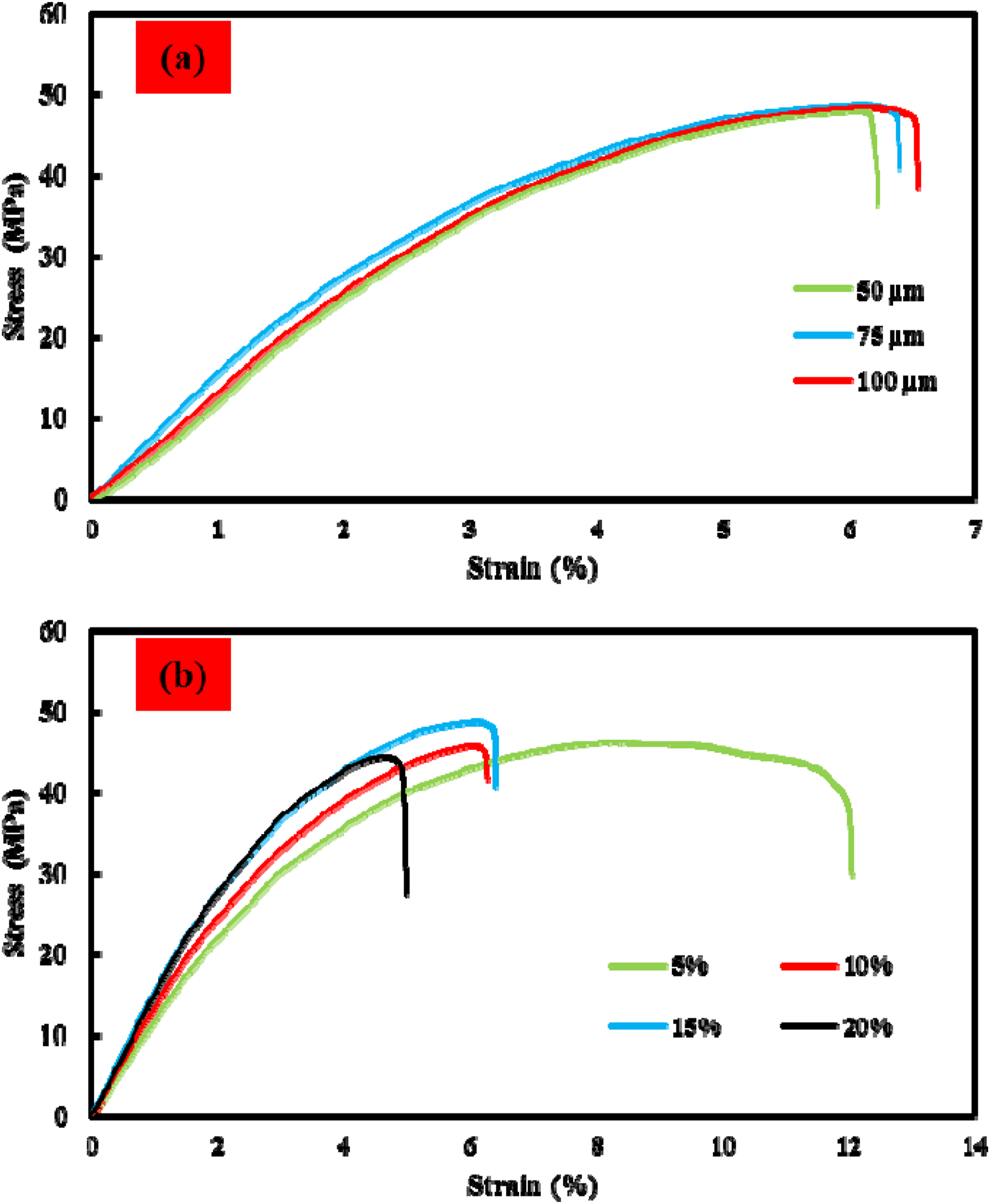

Figure 6(b) shows the stress-strain diagrams to investigate the effect of maple wood fiber content on mechanical properties under bending loading. The results show the superiority of the sample containing 5% in elongation and the composite containing 15% in tensile strength. This trend is consistent with tensile mechanical properties. The bending strength values of these composites are in the range of 44.40 and 48.74 MPa, which respectively the highest and lowest belong to the composites containing 15% and 20% content. The composite containing 20% fiber content, showed the lowest tensile strength and lowest elongation. The lack of proper distribution of fibers is associated with their agglomeration, and these areas of agglomeration prone to join small and micron cracks due to high porosity and are responsible for strength reduction.

Dielectric properties

The study of dielectric characterizations in wood fiber-reinforced polymer composites helps us understand how these materials respond to electrical signals. Several factors can influence these properties, including chemical modifications, frequency of the electric field, temperature changes, fiber content, and fiber length.³⁶ When an alternating electric field is applied to the material, it creates a process called polarization, which helps us identify the dielectric properties. Relative permittivity measures how well a dielectric material can be polarized when exposed to an alternating electromagnetic field.⁴⁸ The dielectric constant (ε′) is the real part of relative permittivity and indicates how effectively the material can store electrical energy and charge.⁴⁹ Additionally, relative permittivity considers energy losses in the material due to conduction. These losses are represented by the loss factor (ε′′), which shows how much electromagnetic energy is converted into heat within an insulator.⁵⁰ Reliable electrical insulation with minimal energy loss is essential for designing effective power systems. Understanding these dielectric properties allows engineers to create better materials for various applications.

Figure 7 illustrates how the dielectric constant (ε′) and loss factor (ε′′) vary for neat polypropylene (PP) and various composites at two distinct high frequencies: 2.45 GHz (in the microwave range) and 915 MHz. This investigation aims to understand the impact of frequency on the dielectric properties of these materials.

Figure 7.

Effect of frequency on dielectric properties of samples: (a) Dielectric constant and (b) Loss factor.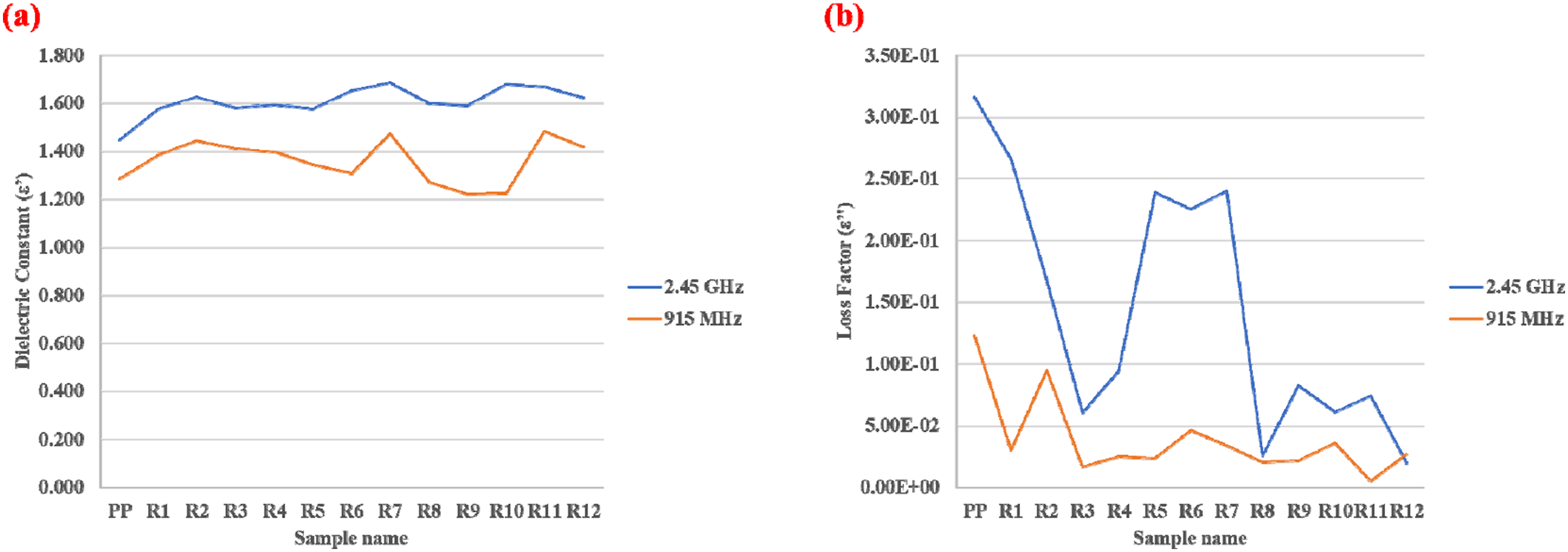

In low-frequency ranges, it is common to observe that as frequency increases, the dielectric constant tends to decrease.⁵¹ This happens because polarization effects become weaker. However, the loss factor can behave differently depending on the material’s composition and structure. As shown in Figure 7, at 2.45 GHz, all samples exhibit a higher dielectric constant and loss factor compared to 915 MHz. This can be explained by the fact that at microwave frequencies, some materials experience stronger polarization effects due to the rapid movement of dipoles.⁵² If the material’s molecular structure allows for effective rotation or alignment of these dipoles in response to the electric field, the dielectric constant can increase. Additionally, the loss factor may rise because more energy is lost as heat from these quick movements. This observation aligns with findings from Khouaja et al,³³ who studied HDPE bio-based composites. Their results show a sudden increase in both dielectric constant and loss factor around 1 GHz in their plots of these properties versus frequency. They noted that when the frequency becomes high, the dipoles cannot keep up with changes in the applied electric field and have less time to align themselves with it. This process is referred to as dipolar relaxation. However, there is a slight increase in response at high frequencies (1 GHz).

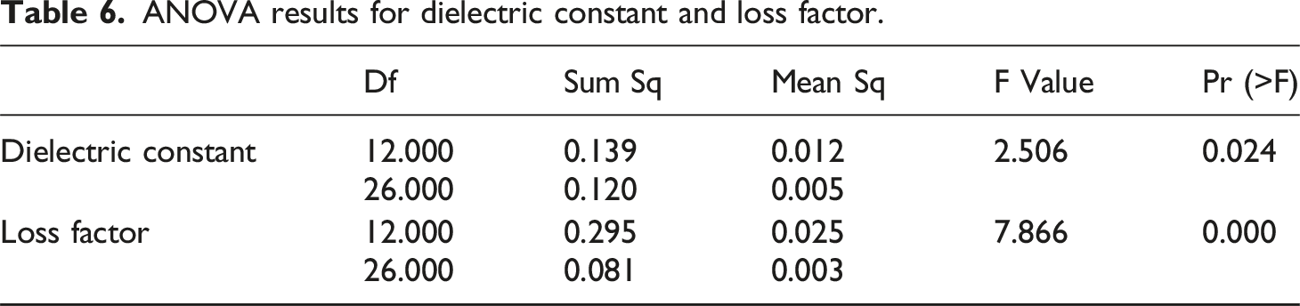
This section will discuss how the volume and length of wood fiber affect the dielectric properties of PP composites. Specifically, we will examine their impact on the dielectric constant (ε′), loss factor (ε′′) and conductivity (σ). To achieve this goal, these parameters are examined at a constant frequency of 2.45 GHz. Additionally, the results of the experiments presented in these sections are analyzed using a statistical method called analysis of variance (ANOVA). ANOVA is used to identify important factors in a study. Its main goal is to determine which parameters significantly affect the measured outcome and to understand their relative importance. This analysis is usually conducted at a 95% confidence level. To evaluate the significance of each parameter, two key values are considered: the F value and the p value. If the p value is less than 0.05, it suggests that the parameter has a significant effect on the outcome.⁵³

Effect on dielectric constant and loss factor

Figure 7(a) shows that all composite samples have a higher dielectric constant than pure PP. This indicates that adding maple wood fiber generally improves the dielectric constant of the samples. The reason for this improvement is that natural fibers introduce polar groups into the non-polar polymer, PP, which increases the dielectric constant. This finding observed in previous studies for HDPE.³³ In Figure 7(b), it can be observed that all composite samples have a lower loss factor than pure PP. A higher dielectric constant and a lower loss factor indicate better dielectric properties for the PP/wood composites compared to pure PP. However, different fiber lengths and concentrations resulted in varying dielectric properties. Among all the composite samples, R1 and R5 had the lowest dielectric constant at 1.58, while sample R7 had the highest at 1.685. The lowest loss factor was found in sample R12 at 0.0201, while sample R1 had the highest loss factor at 0.0266.

Figure 8 illustrates how fiber concentration affects the dielectric constant and loss factor of the samples. The samples are divided into three groups based on fiber length: 50, 75, and 100 µm.

Figure 8.

Effect of wood fiber concentration on dielectric constant and loss factor of composites in constant fiber lengths: (a) 50 µm, (b) 75 µm and (c) 100 µm.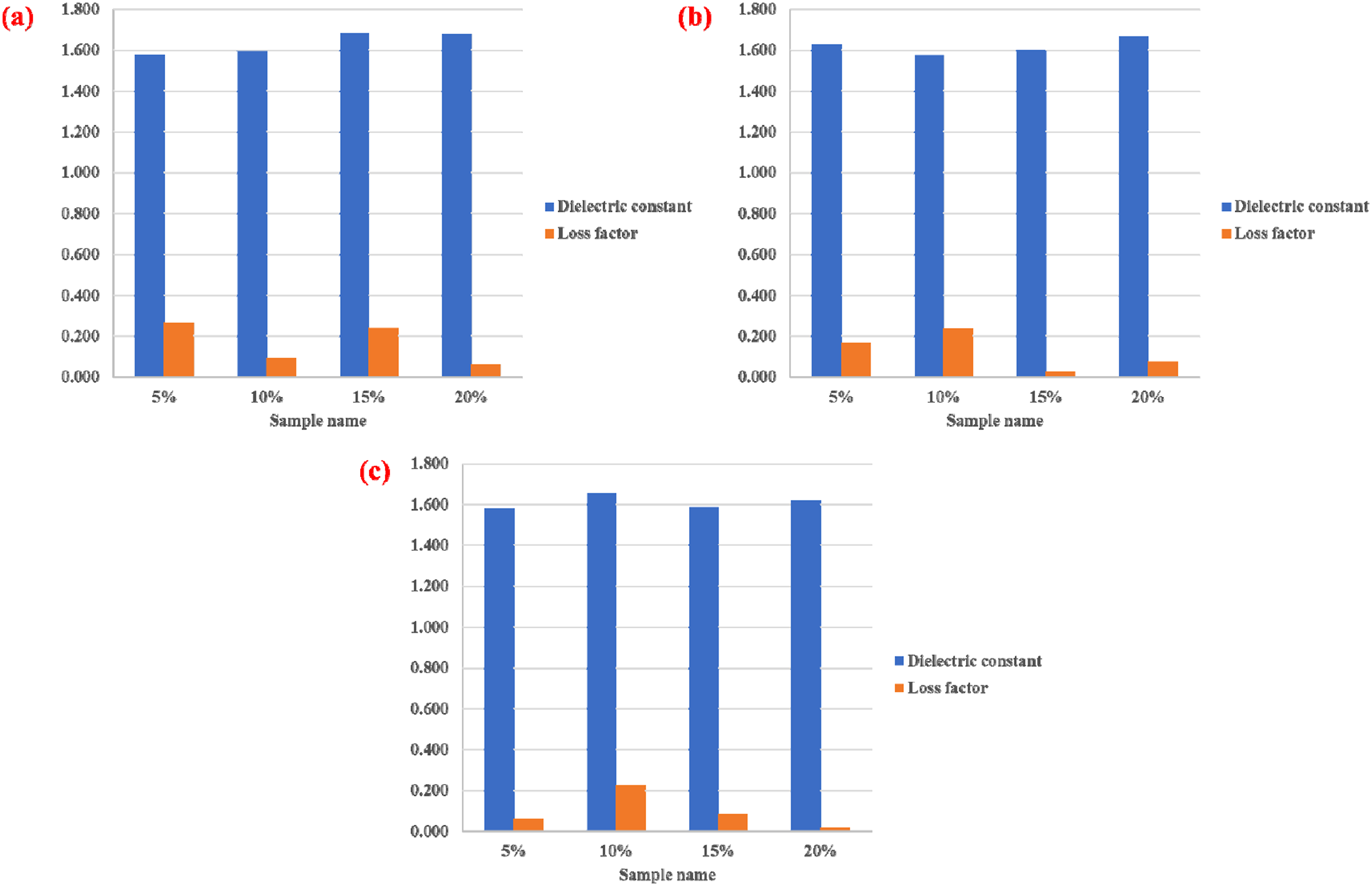

In Figure 8(a), the samples with 50 µm fibers show that the dielectric constant increases as the fiber concentration rises, reaching its peak at 15% concentration. However, at 20%, there is a slight decrease in the dielectric constant. The sample with 15% fiber (R7) has the highest dielectric constant among all samples in this group. The loss factor does not follow a clear trend; the lowest loss factor is seen in the sample with 20% fiber (R10), while the highest is in the sample with 5% fiber (R1).

Figure 8(b) presents samples with 75 µm fibers. Generally, as fiber concentration increases, so does the dielectric constant. However, the sample with 5% fiber stands out by having a higher dielectric constant than those with 10% and 15%. The sample with 10% fiber has the lowest dielectric constant. Similar to the previous group, no distinct trend is observed for the loss factor; however, the sample with 10% fiber has the highest loss factor, while the sample with 15% fiber has the lowest. In fact, there is no linear relationship between the loss parameter and the parameters considered for composite manufacturing (fiber length and fiber volume).

Figure 8(c) shows samples with 100 µm fibers. In this case, as fiber concentration increases, the dielectric constant also generally increases. However, the sample with 10% fiber has both the highest dielectric constant and the highest loss factor in this group. The sample with 20% fiber exhibits the lowest loss factor.

Overall, it can be concluded that as fiber concentration increases, the dielectric constant tends to increase while the loss factor tends to decrease. As mentioned earlier, this improvement is due to the fact that natural fibers introduce polar groups into the non-polar polymer. This addition enhances the dielectric constant of the material. This finding is in good agreement with previous findings.^54–56

Figure 9 illustrates how fiber length affects the dielectric constant and loss factor of composites at constant fiber concentrations (5%, 10%, 15%, and 20%).

Figure 9.

Effect of wood fiber length on dielectric constant and loss factor of composites in constant fiber concentrations: (a) 5%, (b) 10%, (c) 15% and (d) 20%.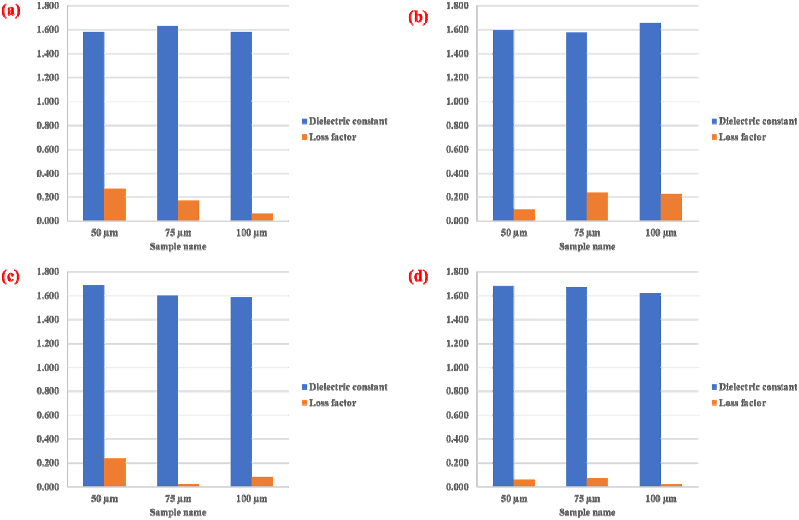

In Figure 9(a), it is evident that the sample with 75 µm fibers has the highest dielectric constant among the samples with 5% fiber concentration. The samples with 50 µm and 100 µm fibers show similar dielectric constants. Regarding the loss factor, as fiber length increases, the loss factor decreases.

In Figure 9(b), for samples with 10% fiber concentration, the trend for the loss factor is different. Here, as fiber length increases, the loss factor also increases. In terms of dielectric constant, the sample with 75 µm fibers has the lowest value, while the sample with 100 µm fibers has the highest.

Figure 9(c) shows that for samples with 15% fiber concentration, as fiber length increases, the dielectric constant decreases. The sample with 75 µm fibers has the lowest loss factor, while the highest loss factor is associated with the sample containing 5% fibers.

In Figure 9(d), for samples with 20% fiber concentration, there is a decreasing trend in dielectric constant as fiber length increases. However, the sample with 75 µm fibers has the highest loss factor, while the sample with 100 µm fibers has the lowest loss factor.

It can be observed from Figure 9 that the effect of fiber length on dielectric constant and loss factor does not follow a consistent trend across different fiber concentrations.

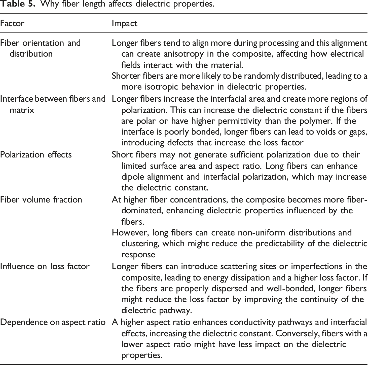
Fiber length can significantly influence the dielectric constant and loss factor due to various effects, which vary with different concentrations. The key points regarding these effects are summarized in the Table 5.

Table 5.

Why fiber length affects dielectric properties.

Factor	Impact
Fiber orientation and distribution	Longer fibers tend to align more during processing and this alignment can create anisotropy in the composite, affecting how electrical fields interact with the material.
Fiber orientation and distribution	Shorter fibers are more likely to be randomly distributed, leading to a more isotropic behavior in dielectric properties.
Interface between fibers and matrix	Longer fibers increase the interfacial area and create more regions of polarization. This can increase the dielectric constant if the fibers are polar or have higher permittivity than the polymer. If the interface is poorly bonded, longer fibers can lead to voids or gaps, introducing defects that increase the loss factor
Polarization effects	Short fibers may not generate sufficient polarization due to their limited surface area and aspect ratio. Long fibers can enhance dipole alignment and interfacial polarization, which may increase the dielectric constant.
Fiber volume fraction	At higher fiber concentrations, the composite becomes more fiber-dominated, enhancing dielectric properties influenced by the fibers.
Fiber volume fraction	However, long fibers can create non-uniform distributions and clustering, which might reduce the predictability of the dielectric response
Influence on loss factor	Longer fibers can introduce scattering sites or imperfections in the composite, leading to energy dissipation and a higher loss factor. If the fibers are properly dispersed and well-bonded, longer fibers might reduce the loss factor by improving the continuity of the dielectric pathway.
Dependence on aspect ratio	A higher aspect ratio enhances conductivity pathways and interfacial effects, increasing the dielectric constant. Conversely, fibers with a lower aspect ratio might have less impact on the dielectric properties.

The results of the ANOVA analysis, which identifies the parameters that significantly affect the dielectric constant and loss factor, are presented in Table 6. The analysis shows that the p-value for dielectric constant is 0.024 and for loss factor is 0, which are less than 0.05. This indicates that there is a significant difference between the groups in the experiment. The boxplots for these two parameters are also presented in Figure 10. Tukey’s HSD (Honestly Significant Difference) test is a statistical method used after an ANOVA to identify which specific group means are significantly different from each other. It compares all possible pairs of means to determine if their differences are greater than what would be expected by chance. The results of Tukey’s HSD test for dielectric constant and loss factor are also presented in Tables A1 and A2 in appendix.

Table 6.

ANOVA results for dielectric constant and loss factor.

	Df	Sum Sq	Mean Sq	F Value	Pr (>F)
Dielectric constant	12.000	0.139	0.012	2.506	0.024
Dielectric constant	26.000	0.120	0.005
Loss factor	12.000	0.295	0.025	7.866	0.000
Loss factor	26.000	0.081	0.003

Figure 10.

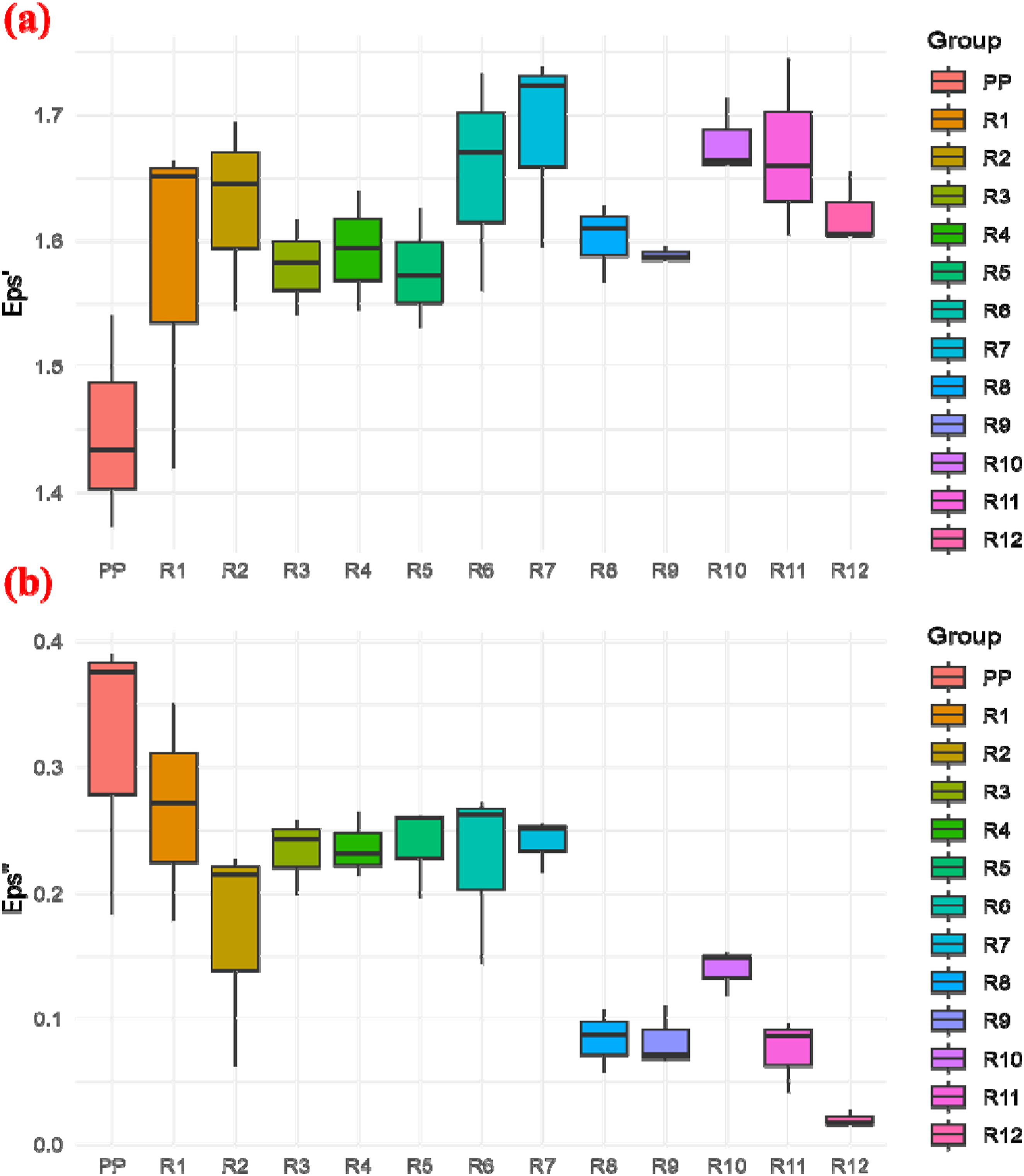
Box Plots for (a) dielectric constant and (b) loss factor.

The results of Tukey’s HSD test for dielectric constant and loss factor for 915 MHz frequency are also presented in Table A3 and A4 in appendix.

Effect on conductivity

Although dielectric materials typically have high resistivity, they can exhibit some conductivity, especially at high frequencies. Conductivity measures how well a material can conduct electric current. Dipolar and interfacial polarization are related to conduction, even with low levels of polarization.⁵⁷ While dipolar molecules are mainly associated with polarization and dielectric constant, they also play a role in electrical conduction. Figure 11 displays the conductivity of all samples at frequencies of 915 MHz and 2.45 GHz. It shows that conductivity increases as frequency rises. At high frequencies, this increase in conductivity is due to electronic polarization and the movement of charge carriers.³³ Additionally, the composite samples generally show higher conductivity than pure polypropylene (PP). The most conductive sample is R7, which contains 15% fiber with a fiber length of 50 µm. In contrast, the sample with the lowest conductivity is R9, which contains 15% fiber with a fiber length of 100 µm.

Figure 11.

Conductivity for pure PP and its composites.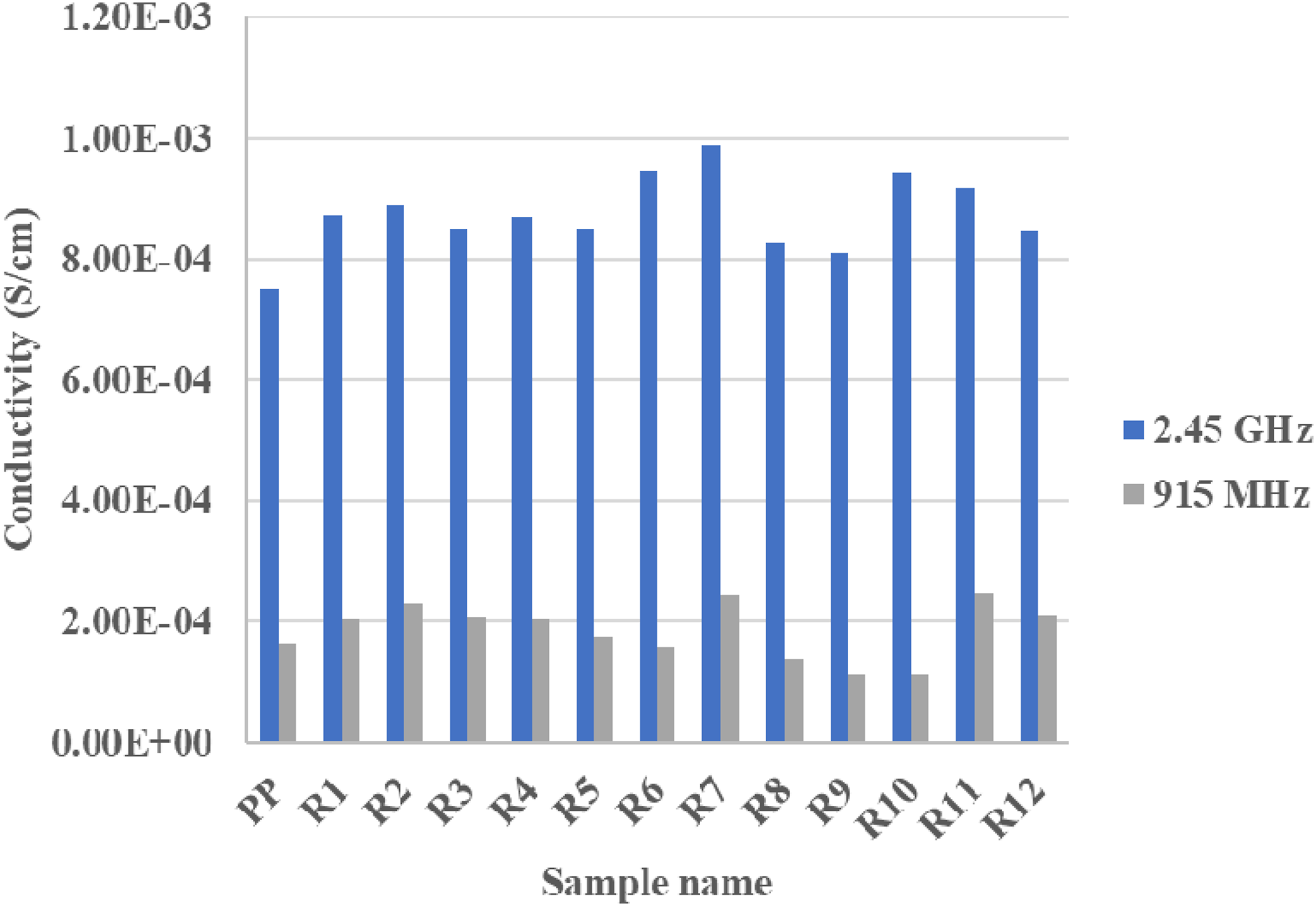

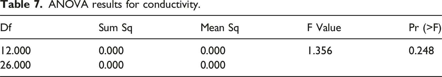
The results of the ANOVA analysis for conductivity, are presented in Table 7. The analysis shows that the p-value for conductivity is 0.248 which is greater than 0.05. This indicates that there is no significant difference between the groups in the experiment. The boxplots for these two parameters are also presented in Figure 12. The results of Tukey’s HSD test for conductivity are also presented in Table A5.

Table 7.

ANOVA results for conductivity.

Df	Sum Sq	Mean Sq	F Value	Pr (>F)
12.000	0.000	0.000	1.356	0.248
26.000	0.000	0.000

Figure 12.

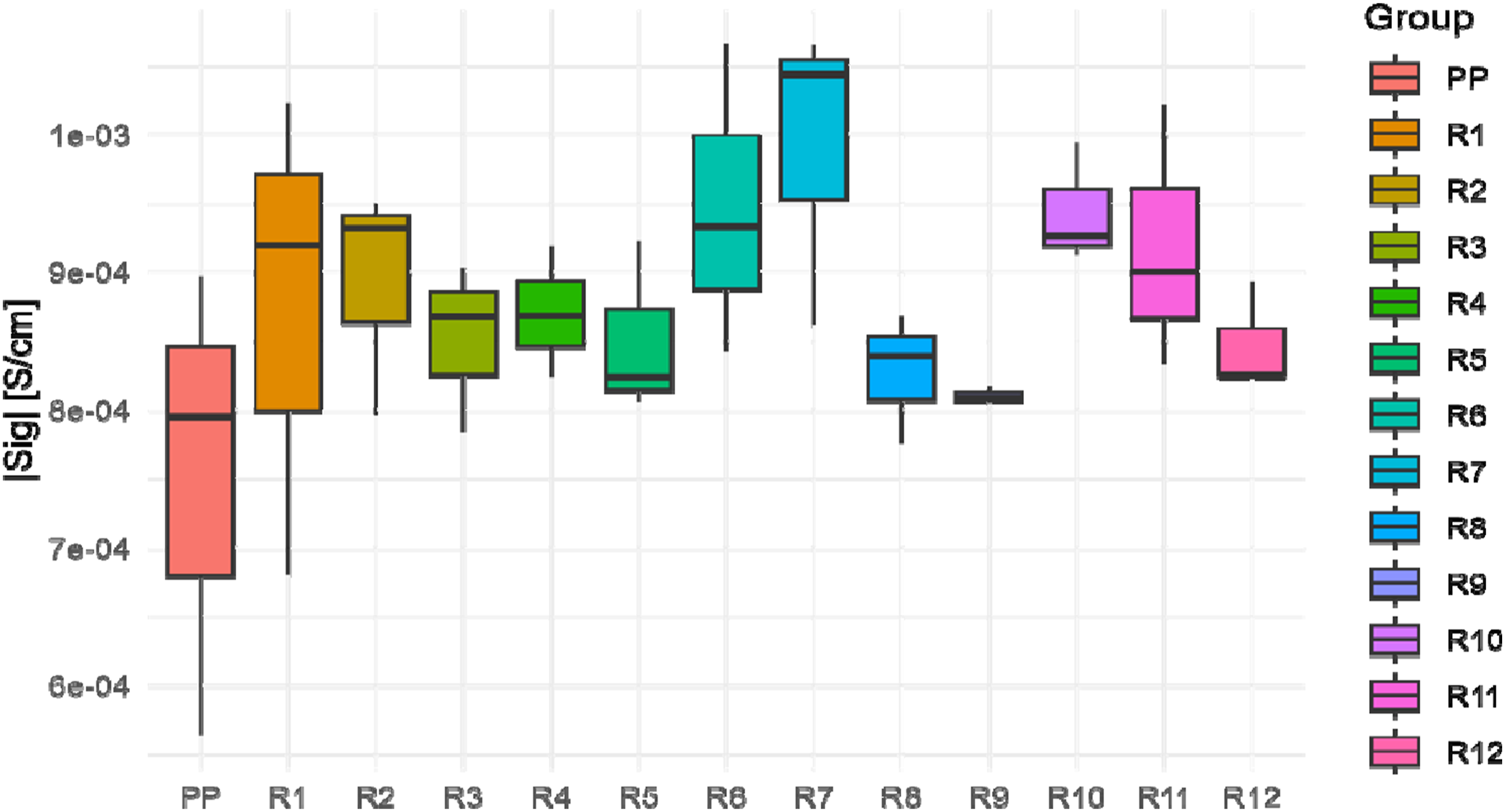
Box Plots for conductivity.

The results of Tukey’s HSD test for conductivity for 915 MHz frequency are also presented in Table A6 in appendix.

Morphology

In the Figure 13, the SEM images of the fracture surfaces of PP matrix composites reinforced with maple wood fiber are demonstrated to investigate its distribution and strengthening effect. According to Figure 13(a), the PP-Maple wood composite containing 5% by weight has a completely uniform and suitable distribution in the matrix.

Figure 13.

SEM images of polypropylene composites reinforced with: (a) 5% by weight and (b) 20% by weight of maple wood fibers.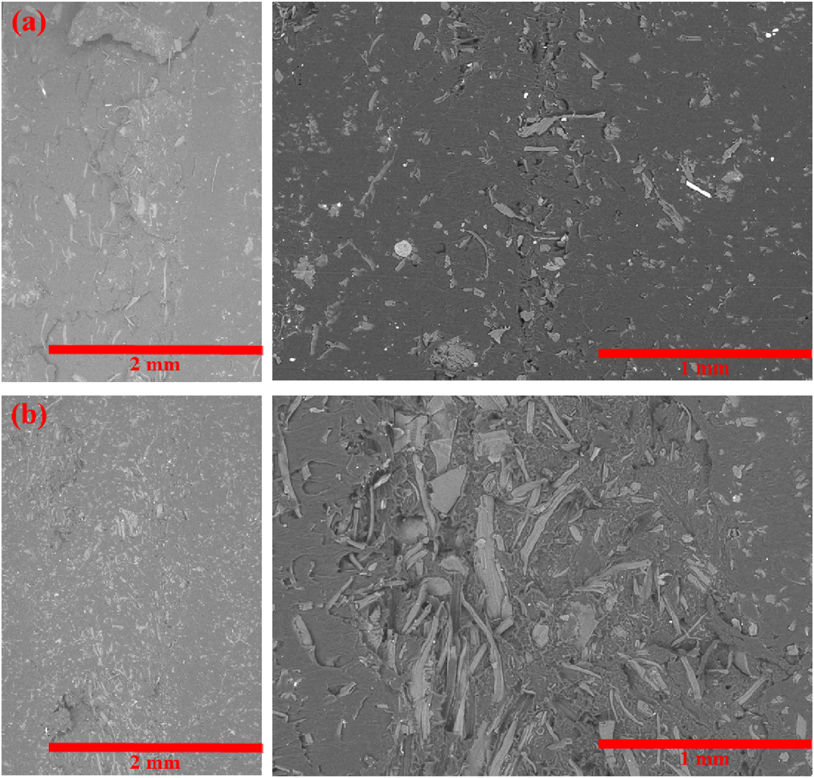

In Figure 13(b), the weight percentage of the maple wood reinforcement has reached 20%, which, compared to Figure 13(a), represents a quadrupling of the volume of the reinforcement in the polymer matrix. According to Figure 13(b), the increase in the volume of the maple wood reinforcement is quite evident and it is also observed in the areas of accumulation and clustering. In fact, these areas rich in reinforcement are the same points that not only do not have a reinforcing role, but also cause a decrease in strength.

This uniform distribution can play a decisive role in increasing the mechanical properties. In fact, with the increase of the reinforcement, the mechanical properties increase, provided that a balance is created between the uniform distribution and the volume of the reinforcement. Therefore, there is an optimal value of reinforcement volume to achieve maximum mechanical properties, and that point, from the microstructural point of view, is the uniform and homogeneous distribution.

Figure 14 shows the SEM images to investigate the role of the fiber length of maple on their distribution in PP matrix. In Figure 14(a), the composite contains 15% by weight of maple wood with a length of 50 μm, and the distribution of fibers is almost uniform and homogeneous. In addition to the volume of the reinforcement discussed in the previous section, the geometry of the reinforcement strongly affects the distribution and this factor also has a very decisive role in improving the mechanical properties. In Figure 14, the distribution of fibers in a polymer matrix with a length of 100 μm can be seen. According to these images, it can be seen that with the increase in the length of the fibers from 50 μm to 100 μm, the distribution of the fibers has changed drastically in a way that in Figure 14(a), a uniform and homogeneous distribution is observed, but in Figure 14(b), this homogeneity is disturbed, and in

Figure 14.

SEM images of polypropylene composites reinforced with maple wood fibers with different fiber length: (a) 50 μm and (b) 100 μm.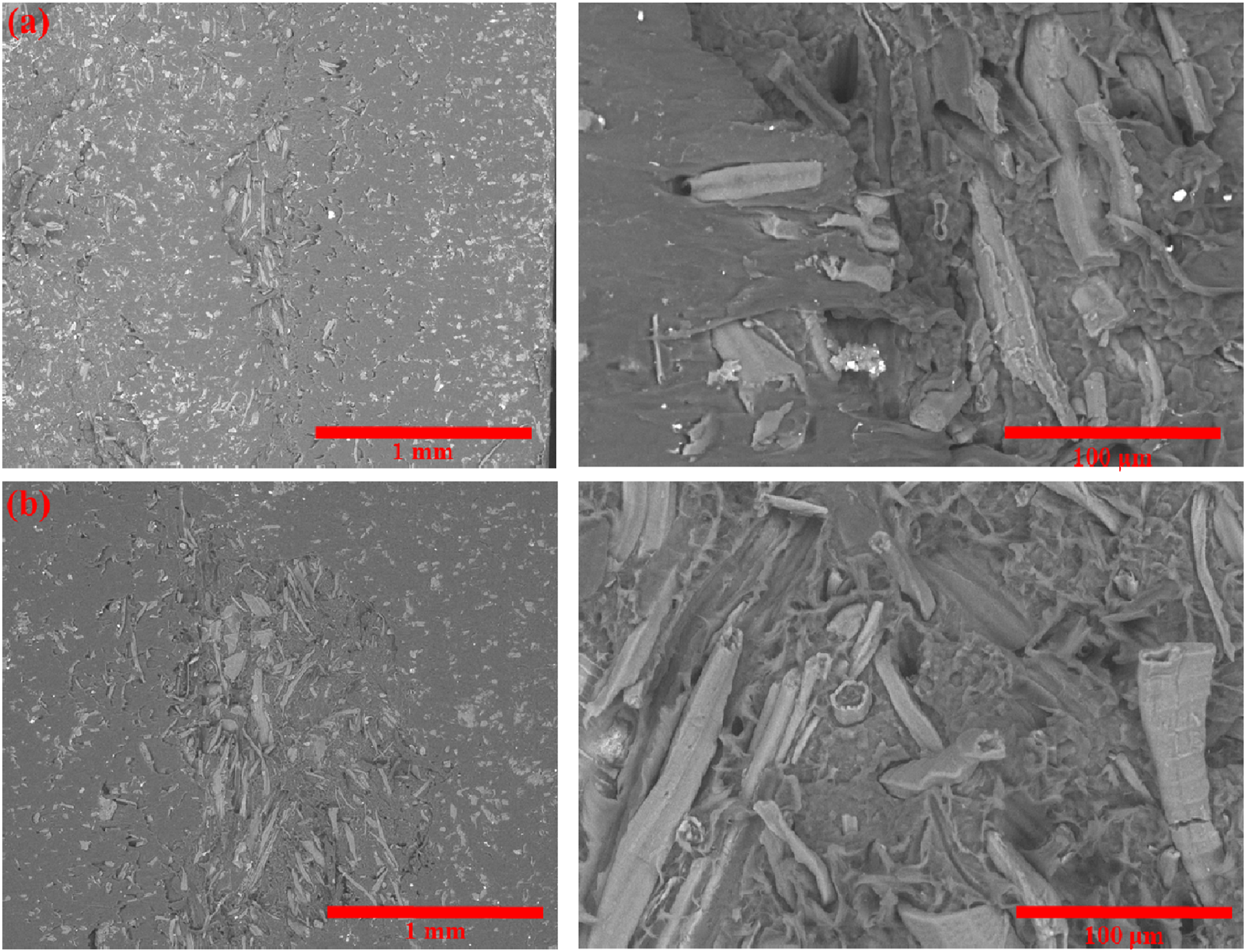

some areas, there are more fibers. In addition to weakening the mechanical properties, this non-uniform distribution causes microstructural and mechanical anisotropy in the composite. The areas containing clustered fiber play the most role in weakening the mechanical properties because the points are full of porosity and empty space and the areas are prone to crack growth and propagation and then failure at a lower stress level.

Conclusion

This study investigated the effects of fiber concentration and fiber length on the mechanical, thermal, and dielectric properties of PP reinforced with maple wood fibers.

• Longer fibers promoted exothermic reactions during crystallization, and increasing fiber concentration reduced peak depth without appreciably changing crystallization temperature, according to DSC results. These findings demonstrated that although fiber length and concentration affect the thermal properties of PP/wood composites, they did not significantly change the overall thermal behavior.

• TGA revealed that the addition of fibers to PP composites affects their thermal stability and degradation behavior; longer fibers reduced IDT and thermal stability, while shorter fibers enhanced residual weight after degradation. Additionally, increasing fiber concentration leads to earlier degradation at lower temperatures, with composites exhibiting greater stability at higher temperatures compared to pure PP.

• The tensile strength of polypropylene composites showed minimal variation with fiber length, with ultimate tensile strengths of 26.46 MPa (50 μm), 27.13 MPa (75 μm), and 25.20 MPa (100 μm). Increasing fiber content from 5% to 15% enhanced tensile strength and Young’s modulus, while elongation decreased. However, beyond 15%, increasing fiber content to 20% resulted in a significant drop in tensile strength to 19.89 MPa due to poor fiber distribution.

• The composites demonstrated comparable mechanical performance under three-point bending at varying fiber lengths, with bending strengths ranging from 44.40 MPa (20% content) to 48.74 MPa (15% content). Because of fiber accumulation and high porosity that causes cracks, the sample with 5% fiber content exhibits the highest elongation while the composite with 20% fiber content exhibits the lowest tensile strength and elongation.

• The SEM results proved that the distribution of maple wood fibers in polypropylene (PP) composites has a major impact on mechanical properties; a uniform distribution at 5% weight improves strength, whereas clustering at 20% weight weakens the composite. Furthermore, homogeneity was disrupted by increasing the fiber length from 50 μm to 100 μm, which resulted in microstructural anisotropy and lowers mechanical performance because of porosity and possible crack propagation.

• The addition of wood fibers enhanced the dielectric constant (ε′) while reducing the loss factor (ε′′), indicating improved dielectric properties compared to pure PP. This enhancement is attributed to the introduction of polar groups from natural fibers, which facilitate better polarization in the material.

• The study proved that dielectric properties vary significantly with frequency, fiber concentration, and fiber length. At higher frequencies (2.45 GHz), materials exhibit stronger polarization effects, resulting in higher dielectric constants and loss factors. Additionally, the relationship between fiber length and dielectric properties was complex, showing inconsistent trends across different fiber concentrations. Furthermore, as fiber concentration increased, the dielectric constant tends to increase while the loss factor tends to decrease.

Footnotes

Author contributions

All authors contributed to the investigation, conceptualization, and analysis of the information in this manuscript, and were involved in the writing process.

Declaration of conflicting interests

The author(s) declared no potential conflicts of interest with respect to the research, authorship, and/or publication of this article.

Funding

The author(s) disclosed receipt of the following financial support for the research, authorship, and/or publication of this article: “The authors express their gratitude to the Fondation J.A. DeSève and the Fondation de l’UQAT for their financial support.”

Ethical statement

ORCID iD

Farshid Basiji

Appendix

Table A1.

Tukey’s HSD test for dielectric constant in 2.45 GHz.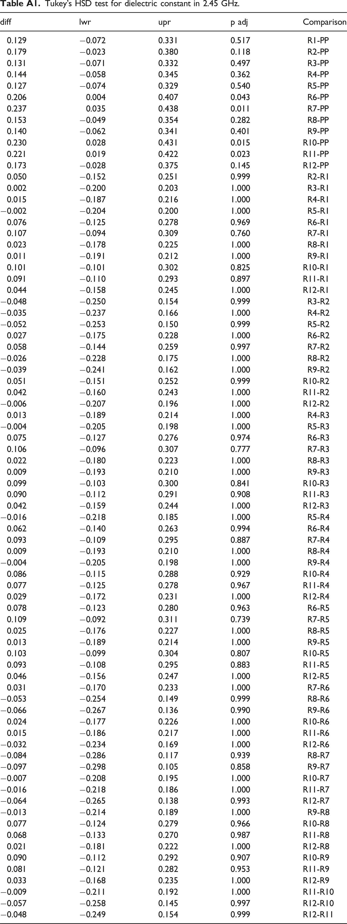

diff	lwr	upr	p adj	Comparison
0.129	−0.072	0.331	0.517	R1-PP
0.179	−0.023	0.380	0.118	R2-PP
0.131	−0.071	0.332	0.497	R3-PP
0.144	−0.058	0.345	0.362	R4-PP
0.127	−0.074	0.329	0.540	R5-PP
0.206	0.004	0.407	0.043	R6-PP
0.237	0.035	0.438	0.011	R7-PP
0.153	−0.049	0.354	0.282	R8-PP
0.140	−0.062	0.341	0.401	R9-PP
0.230	0.028	0.431	0.015	R10-PP
0.221	0.019	0.422	0.023	R11-PP
0.173	−0.028	0.375	0.145	R12-PP
0.050	−0.152	0.251	0.999	R2-R1
0.002	−0.200	0.203	1.000	R3-R1
0.015	−0.187	0.216	1.000	R4-R1
−0.002	−0.204	0.200	1.000	R5-R1
0.076	−0.125	0.278	0.969	R6-R1
0.107	−0.094	0.309	0.760	R7-R1
0.023	−0.178	0.225	1.000	R8-R1
0.011	−0.191	0.212	1.000	R9-R1
0.101	−0.101	0.302	0.825	R10-R1
0.091	−0.110	0.293	0.897	R11-R1
0.044	−0.158	0.245	1.000	R12-R1
−0.048	−0.250	0.154	0.999	R3-R2
−0.035	−0.237	0.166	1.000	R4-R2
−0.052	−0.253	0.150	0.999	R5-R2
0.027	−0.175	0.228	1.000	R6-R2
0.058	−0.144	0.259	0.997	R7-R2
−0.026	−0.228	0.175	1.000	R8-R2
−0.039	−0.241	0.162	1.000	R9-R2
0.051	−0.151	0.252	0.999	R10-R2
0.042	−0.160	0.243	1.000	R11-R2
−0.006	−0.207	0.196	1.000	R12-R2
0.013	−0.189	0.214	1.000	R4-R3
−0.004	−0.205	0.198	1.000	R5-R3
0.075	−0.127	0.276	0.974	R6-R3
0.106	−0.096	0.307	0.777	R7-R3
0.022	−0.180	0.223	1.000	R8-R3
0.009	−0.193	0.210	1.000	R9-R3
0.099	−0.103	0.300	0.841	R10-R3
0.090	−0.112	0.291	0.908	R11-R3
0.042	−0.159	0.244	1.000	R12-R3
−0.016	−0.218	0.185	1.000	R5-R4
0.062	−0.140	0.263	0.994	R6-R4
0.093	−0.109	0.295	0.887	R7-R4
0.009	−0.193	0.210	1.000	R8-R4
−0.004	−0.205	0.198	1.000	R9-R4
0.086	−0.115	0.288	0.929	R10-R4
0.077	−0.125	0.278	0.967	R11-R4
0.029	−0.172	0.231	1.000	R12-R4
0.078	−0.123	0.280	0.963	R6-R5
0.109	−0.092	0.311	0.739	R7-R5
0.025	−0.176	0.227	1.000	R8-R5
0.013	−0.189	0.214	1.000	R9-R5
0.103	−0.099	0.304	0.807	R10-R5
0.093	−0.108	0.295	0.883	R11-R5
0.046	−0.156	0.247	1.000	R12-R5
0.031	−0.170	0.233	1.000	R7-R6
−0.053	−0.254	0.149	0.999	R8-R6
−0.066	−0.267	0.136	0.990	R9-R6
0.024	−0.177	0.226	1.000	R10-R6
0.015	−0.186	0.217	1.000	R11-R6
−0.032	−0.234	0.169	1.000	R12-R6
−0.084	−0.286	0.117	0.939	R8-R7
−0.097	−0.298	0.105	0.858	R9-R7
−0.007	−0.208	0.195	1.000	R10-R7
−0.016	−0.218	0.186	1.000	R11-R7
−0.064	−0.265	0.138	0.993	R12-R7
−0.013	−0.214	0.189	1.000	R9-R8
0.077	−0.124	0.279	0.966	R10-R8
0.068	−0.133	0.270	0.987	R11-R8
0.021	−0.181	0.222	1.000	R12-R8
0.090	−0.112	0.292	0.907	R10-R9
0.081	−0.121	0.282	0.953	R11-R9
0.033	−0.168	0.235	1.000	R12-R9
−0.009	−0.211	0.192	1.000	R11-R10
−0.057	−0.258	0.145	0.997	R12-R10
−0.048	−0.249	0.154	0.999	R12-R11

Table A2.

Tukey’s HSD test for loss factor in 2.45 GHz.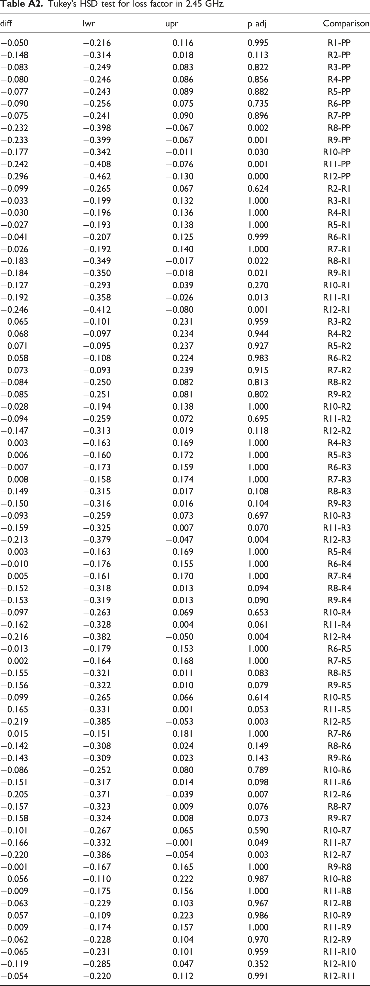

diff	lwr	upr	p adj	Comparison
−0.050	−0.216	0.116	0.995	R1-PP
−0.148	−0.314	0.018	0.113	R2-PP
−0.083	−0.249	0.083	0.822	R3-PP
−0.080	−0.246	0.086	0.856	R4-PP
−0.077	−0.243	0.089	0.882	R5-PP
−0.090	−0.256	0.075	0.735	R6-PP
−0.075	−0.241	0.090	0.896	R7-PP
−0.232	−0.398	−0.067	0.002	R8-PP
−0.233	−0.399	−0.067	0.001	R9-PP
−0.177	−0.342	−0.011	0.030	R10-PP
−0.242	−0.408	−0.076	0.001	R11-PP
−0.296	−0.462	−0.130	0.000	R12-PP
−0.099	−0.265	0.067	0.624	R2-R1
−0.033	−0.199	0.132	1.000	R3-R1
−0.030	−0.196	0.136	1.000	R4-R1
−0.027	−0.193	0.138	1.000	R5-R1
−0.041	−0.207	0.125	0.999	R6-R1
−0.026	−0.192	0.140	1.000	R7-R1
−0.183	−0.349	−0.017	0.022	R8-R1
−0.184	−0.350	−0.018	0.021	R9-R1
−0.127	−0.293	0.039	0.270	R10-R1
−0.192	−0.358	−0.026	0.013	R11-R1
−0.246	−0.412	−0.080	0.001	R12-R1
0.065	−0.101	0.231	0.959	R3-R2
0.068	−0.097	0.234	0.944	R4-R2
0.071	−0.095	0.237	0.927	R5-R2
0.058	−0.108	0.224	0.983	R6-R2
0.073	−0.093	0.239	0.915	R7-R2
−0.084	−0.250	0.082	0.813	R8-R2
−0.085	−0.251	0.081	0.802	R9-R2
−0.028	−0.194	0.138	1.000	R10-R2
−0.094	−0.259	0.072	0.695	R11-R2
−0.147	−0.313	0.019	0.118	R12-R2
0.003	−0.163	0.169	1.000	R4-R3
0.006	−0.160	0.172	1.000	R5-R3
−0.007	−0.173	0.159	1.000	R6-R3
0.008	−0.158	0.174	1.000	R7-R3
−0.149	−0.315	0.017	0.108	R8-R3
−0.150	−0.316	0.016	0.104	R9-R3
−0.093	−0.259	0.073	0.697	R10-R3
−0.159	−0.325	0.007	0.070	R11-R3
−0.213	−0.379	−0.047	0.004	R12-R3
0.003	−0.163	0.169	1.000	R5-R4
−0.010	−0.176	0.155	1.000	R6-R4
0.005	−0.161	0.170	1.000	R7-R4
−0.152	−0.318	0.013	0.094	R8-R4
−0.153	−0.319	0.013	0.090	R9-R4
−0.097	−0.263	0.069	0.653	R10-R4
−0.162	−0.328	0.004	0.061	R11-R4
−0.216	−0.382	−0.050	0.004	R12-R4
−0.013	−0.179	0.153	1.000	R6-R5
0.002	−0.164	0.168	1.000	R7-R5
−0.155	−0.321	0.011	0.083	R8-R5
−0.156	−0.322	0.010	0.079	R9-R5
−0.099	−0.265	0.066	0.614	R10-R5
−0.165	−0.331	0.001	0.053	R11-R5
−0.219	−0.385	−0.053	0.003	R12-R5
0.015	−0.151	0.181	1.000	R7-R6
−0.142	−0.308	0.024	0.149	R8-R6
−0.143	−0.309	0.023	0.143	R9-R6
−0.086	−0.252	0.080	0.789	R10-R6
−0.151	−0.317	0.014	0.098	R11-R6
−0.205	−0.371	−0.039	0.007	R12-R6
−0.157	−0.323	0.009	0.076	R8-R7
−0.158	−0.324	0.008	0.073	R9-R7
−0.101	−0.267	0.065	0.590	R10-R7
−0.166	−0.332	−0.001	0.049	R11-R7
−0.220	−0.386	−0.054	0.003	R12-R7
−0.001	−0.167	0.165	1.000	R9-R8
0.056	−0.110	0.222	0.987	R10-R8
−0.009	−0.175	0.156	1.000	R11-R8
−0.063	−0.229	0.103	0.967	R12-R8
0.057	−0.109	0.223	0.986	R10-R9
−0.009	−0.174	0.157	1.000	R11-R9
−0.062	−0.228	0.104	0.970	R12-R9
−0.065	−0.231	0.101	0.959	R11-R10
−0.119	−0.285	0.047	0.352	R12-R10
−0.054	−0.220	0.112	0.991	R12-R11

Table A3.

Tukey’s HSD test for dielectric constant in 915 MHz.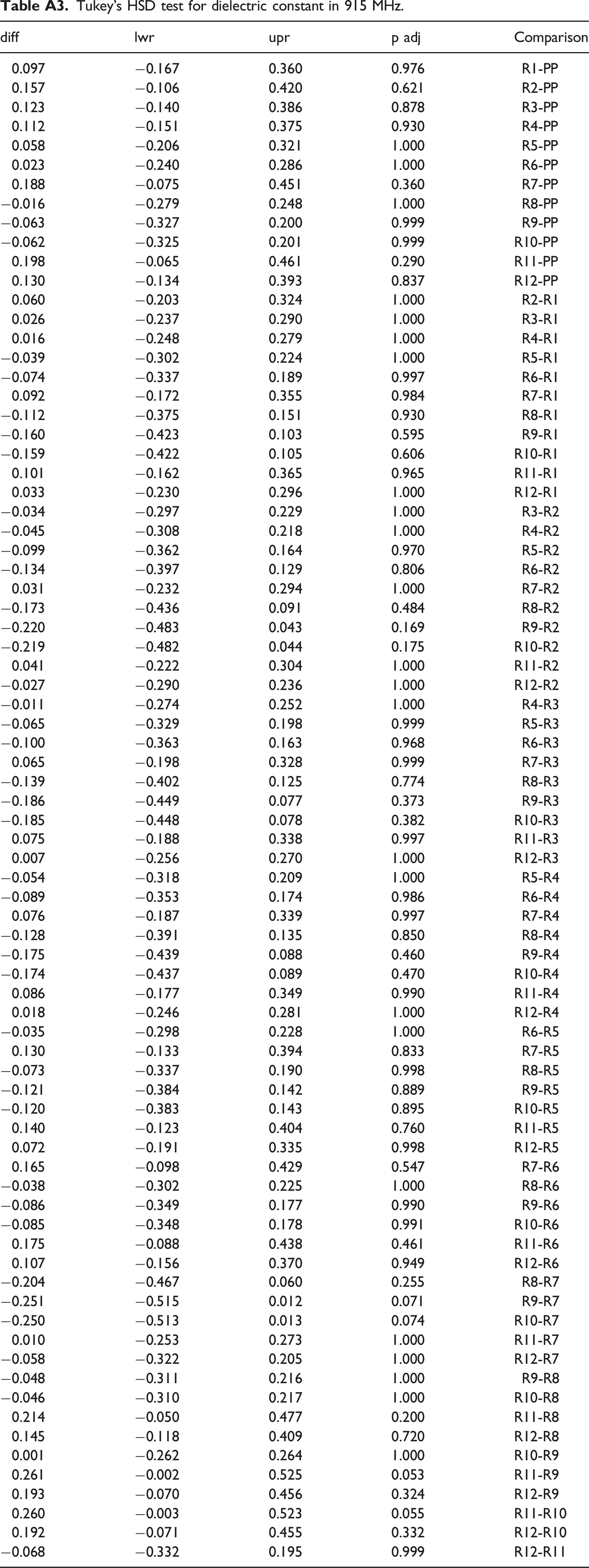

diff	lwr	upr	p adj	Comparison
0.097	−0.167	0.360	0.976	R1-PP
0.157	−0.106	0.420	0.621	R2-PP
0.123	−0.140	0.386	0.878	R3-PP
0.112	−0.151	0.375	0.930	R4-PP
0.058	−0.206	0.321	1.000	R5-PP
0.023	−0.240	0.286	1.000	R6-PP
0.188	−0.075	0.451	0.360	R7-PP
−0.016	−0.279	0.248	1.000	R8-PP
−0.063	−0.327	0.200	0.999	R9-PP
−0.062	−0.325	0.201	0.999	R10-PP
0.198	−0.065	0.461	0.290	R11-PP
0.130	−0.134	0.393	0.837	R12-PP
0.060	−0.203	0.324	1.000	R2-R1
0.026	−0.237	0.290	1.000	R3-R1
0.016	−0.248	0.279	1.000	R4-R1
−0.039	−0.302	0.224	1.000	R5-R1
−0.074	−0.337	0.189	0.997	R6-R1
0.092	−0.172	0.355	0.984	R7-R1
−0.112	−0.375	0.151	0.930	R8-R1
−0.160	−0.423	0.103	0.595	R9-R1
−0.159	−0.422	0.105	0.606	R10-R1
0.101	−0.162	0.365	0.965	R11-R1
0.033	−0.230	0.296	1.000	R12-R1
−0.034	−0.297	0.229	1.000	R3-R2
−0.045	−0.308	0.218	1.000	R4-R2
−0.099	−0.362	0.164	0.970	R5-R2
−0.134	−0.397	0.129	0.806	R6-R2
0.031	−0.232	0.294	1.000	R7-R2
−0.173	−0.436	0.091	0.484	R8-R2
−0.220	−0.483	0.043	0.169	R9-R2
−0.219	−0.482	0.044	0.175	R10-R2
0.041	−0.222	0.304	1.000	R11-R2
−0.027	−0.290	0.236	1.000	R12-R2
−0.011	−0.274	0.252	1.000	R4-R3
−0.065	−0.329	0.198	0.999	R5-R3
−0.100	−0.363	0.163	0.968	R6-R3
0.065	−0.198	0.328	0.999	R7-R3
−0.139	−0.402	0.125	0.774	R8-R3
−0.186	−0.449	0.077	0.373	R9-R3
−0.185	−0.448	0.078	0.382	R10-R3
0.075	−0.188	0.338	0.997	R11-R3
0.007	−0.256	0.270	1.000	R12-R3
−0.054	−0.318	0.209	1.000	R5-R4
−0.089	−0.353	0.174	0.986	R6-R4
0.076	−0.187	0.339	0.997	R7-R4
−0.128	−0.391	0.135	0.850	R8-R4
−0.175	−0.439	0.088	0.460	R9-R4
−0.174	−0.437	0.089	0.470	R10-R4
0.086	−0.177	0.349	0.990	R11-R4
0.018	−0.246	0.281	1.000	R12-R4
−0.035	−0.298	0.228	1.000	R6-R5
0.130	−0.133	0.394	0.833	R7-R5
−0.073	−0.337	0.190	0.998	R8-R5
−0.121	−0.384	0.142	0.889	R9-R5
−0.120	−0.383	0.143	0.895	R10-R5
0.140	−0.123	0.404	0.760	R11-R5
0.072	−0.191	0.335	0.998	R12-R5
0.165	−0.098	0.429	0.547	R7-R6
−0.038	−0.302	0.225	1.000	R8-R6
−0.086	−0.349	0.177	0.990	R9-R6
−0.085	−0.348	0.178	0.991	R10-R6
0.175	−0.088	0.438	0.461	R11-R6
0.107	−0.156	0.370	0.949	R12-R6
−0.204	−0.467	0.060	0.255	R8-R7
−0.251	−0.515	0.012	0.071	R9-R7
−0.250	−0.513	0.013	0.074	R10-R7
0.010	−0.253	0.273	1.000	R11-R7
−0.058	−0.322	0.205	1.000	R12-R7
−0.048	−0.311	0.216	1.000	R9-R8
−0.046	−0.310	0.217	1.000	R10-R8
0.214	−0.050	0.477	0.200	R11-R8
0.145	−0.118	0.409	0.720	R12-R8
0.001	−0.262	0.264	1.000	R10-R9
0.261	−0.002	0.525	0.053	R11-R9
0.193	−0.070	0.456	0.324	R12-R9
0.260	−0.003	0.523	0.055	R11-R10
0.192	−0.071	0.455	0.332	R12-R10
−0.068	−0.332	0.195	0.999	R12-R11

Table A4.

Tukey’s HSD test for loss factor in 915 MHz.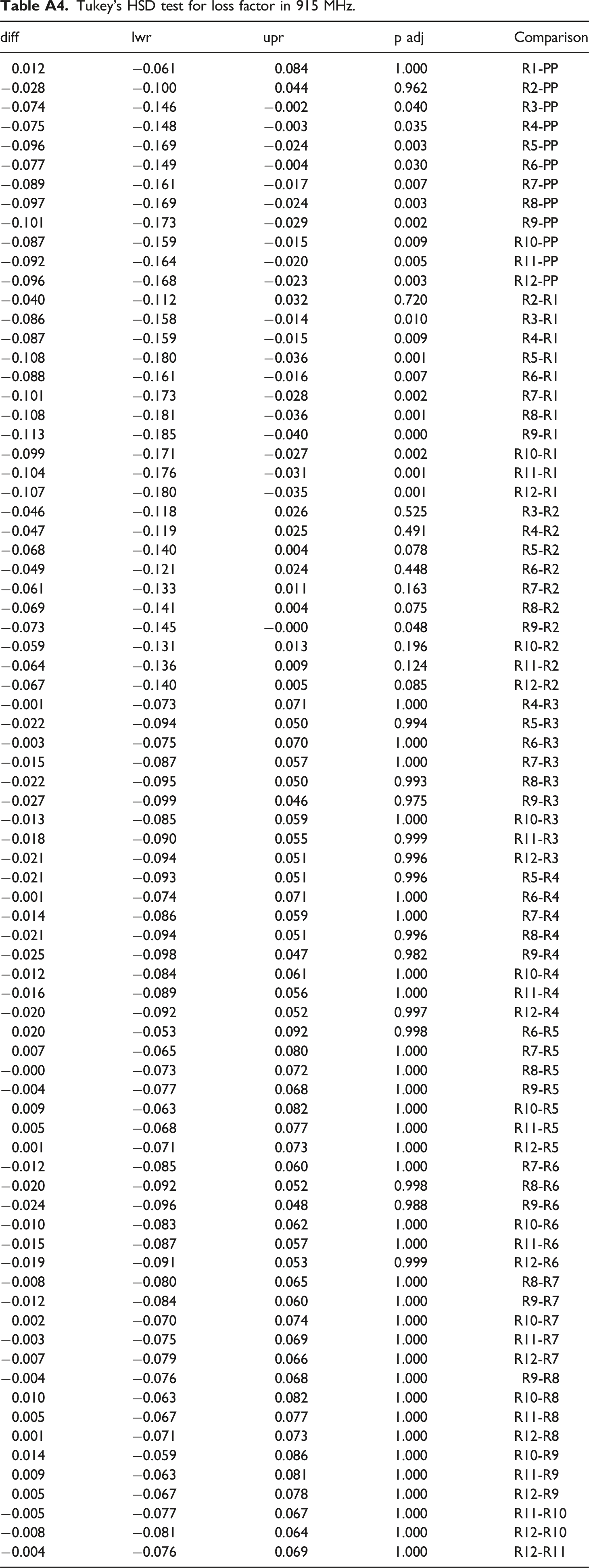

diff	lwr	upr	p adj	Comparison
0.012	−0.061	0.084	1.000	R1-PP
−0.028	−0.100	0.044	0.962	R2-PP
−0.074	−0.146	−0.002	0.040	R3-PP
−0.075	−0.148	−0.003	0.035	R4-PP
−0.096	−0.169	−0.024	0.003	R5-PP
−0.077	−0.149	−0.004	0.030	R6-PP
−0.089	−0.161	−0.017	0.007	R7-PP
−0.097	−0.169	−0.024	0.003	R8-PP
−0.101	−0.173	−0.029	0.002	R9-PP
−0.087	−0.159	−0.015	0.009	R10-PP
−0.092	−0.164	−0.020	0.005	R11-PP
−0.096	−0.168	−0.023	0.003	R12-PP
−0.040	−0.112	0.032	0.720	R2-R1
−0.086	−0.158	−0.014	0.010	R3-R1
−0.087	−0.159	−0.015	0.009	R4-R1
−0.108	−0.180	−0.036	0.001	R5-R1
−0.088	−0.161	−0.016	0.007	R6-R1
−0.101	−0.173	−0.028	0.002	R7-R1
−0.108	−0.181	−0.036	0.001	R8-R1
−0.113	−0.185	−0.040	0.000	R9-R1
−0.099	−0.171	−0.027	0.002	R10-R1
−0.104	−0.176	−0.031	0.001	R11-R1
−0.107	−0.180	−0.035	0.001	R12-R1
−0.046	−0.118	0.026	0.525	R3-R2
−0.047	−0.119	0.025	0.491	R4-R2
−0.068	−0.140	0.004	0.078	R5-R2
−0.049	−0.121	0.024	0.448	R6-R2
−0.061	−0.133	0.011	0.163	R7-R2
−0.069	−0.141	0.004	0.075	R8-R2
−0.073	−0.145	−0.000	0.048	R9-R2
−0.059	−0.131	0.013	0.196	R10-R2
−0.064	−0.136	0.009	0.124	R11-R2
−0.067	−0.140	0.005	0.085	R12-R2
−0.001	−0.073	0.071	1.000	R4-R3
−0.022	−0.094	0.050	0.994	R5-R3
−0.003	−0.075	0.070	1.000	R6-R3
−0.015	−0.087	0.057	1.000	R7-R3
−0.022	−0.095	0.050	0.993	R8-R3
−0.027	−0.099	0.046	0.975	R9-R3
−0.013	−0.085	0.059	1.000	R10-R3
−0.018	−0.090	0.055	0.999	R11-R3
−0.021	−0.094	0.051	0.996	R12-R3
−0.021	−0.093	0.051	0.996	R5-R4
−0.001	−0.074	0.071	1.000	R6-R4
−0.014	−0.086	0.059	1.000	R7-R4
−0.021	−0.094	0.051	0.996	R8-R4
−0.025	−0.098	0.047	0.982	R9-R4
−0.012	−0.084	0.061	1.000	R10-R4
−0.016	−0.089	0.056	1.000	R11-R4
−0.020	−0.092	0.052	0.997	R12-R4
0.020	−0.053	0.092	0.998	R6-R5
0.007	−0.065	0.080	1.000	R7-R5
−0.000	−0.073	0.072	1.000	R8-R5
−0.004	−0.077	0.068	1.000	R9-R5
0.009	−0.063	0.082	1.000	R10-R5
0.005	−0.068	0.077	1.000	R11-R5
0.001	−0.071	0.073	1.000	R12-R5
−0.012	−0.085	0.060	1.000	R7-R6
−0.020	−0.092	0.052	0.998	R8-R6
−0.024	−0.096	0.048	0.988	R9-R6
−0.010	−0.083	0.062	1.000	R10-R6
−0.015	−0.087	0.057	1.000	R11-R6
−0.019	−0.091	0.053	0.999	R12-R6
−0.008	−0.080	0.065	1.000	R8-R7
−0.012	−0.084	0.060	1.000	R9-R7
0.002	−0.070	0.074	1.000	R10-R7
−0.003	−0.075	0.069	1.000	R11-R7
−0.007	−0.079	0.066	1.000	R12-R7
−0.004	−0.076	0.068	1.000	R9-R8
0.010	−0.063	0.082	1.000	R10-R8
0.005	−0.067	0.077	1.000	R11-R8
0.001	−0.071	0.073	1.000	R12-R8
0.014	−0.059	0.086	1.000	R10-R9
0.009	−0.063	0.081	1.000	R11-R9
0.005	−0.067	0.078	1.000	R12-R9
−0.005	−0.077	0.067	1.000	R11-R10
−0.008	−0.081	0.064	1.000	R12-R10
−0.004	−0.076	0.069	1.000	R12-R11

Table A5.

Tukey’s HSD test for conductivity in 2.45 GHz.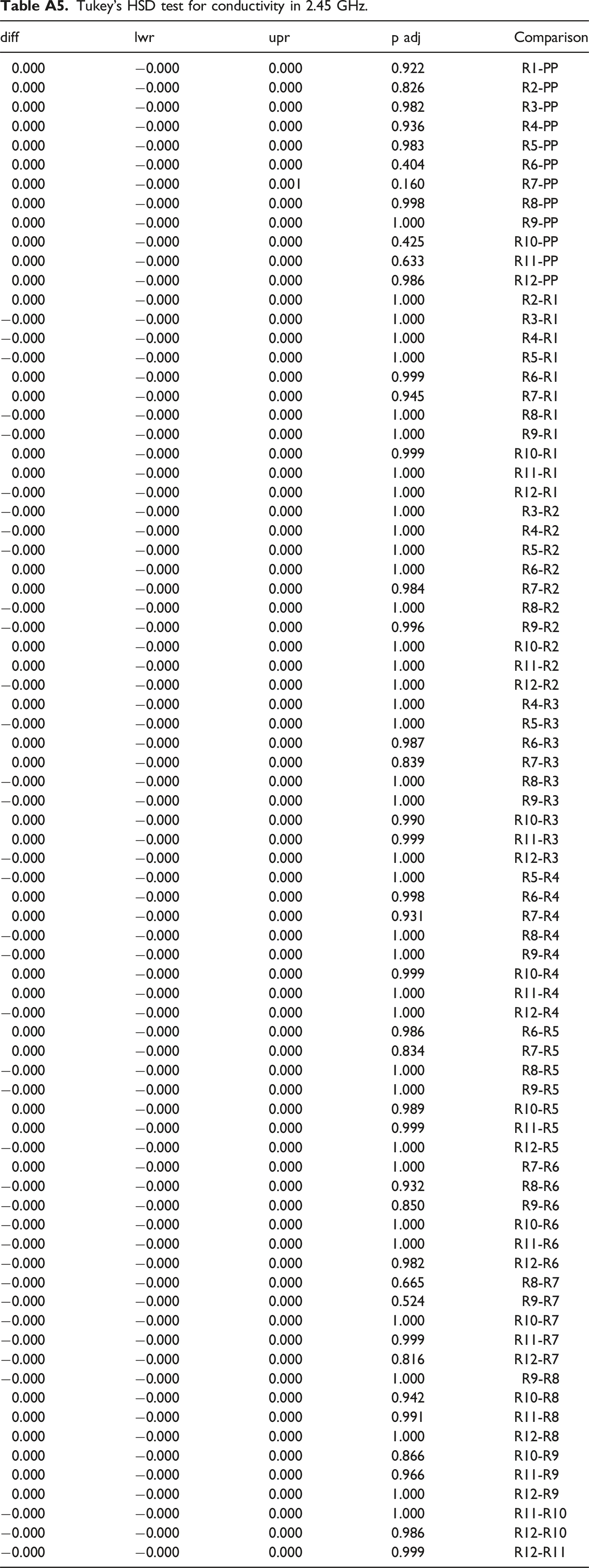

diff	lwr	upr	p adj	Comparison
0.000	−0.000	0.000	0.922	R1-PP
0.000	−0.000	0.000	0.826	R2-PP
0.000	−0.000	0.000	0.982	R3-PP
0.000	−0.000	0.000	0.936	R4-PP
0.000	−0.000	0.000	0.983	R5-PP
0.000	−0.000	0.000	0.404	R6-PP
0.000	−0.000	0.001	0.160	R7-PP
0.000	−0.000	0.000	0.998	R8-PP
0.000	−0.000	0.000	1.000	R9-PP
0.000	−0.000	0.000	0.425	R10-PP
0.000	−0.000	0.000	0.633	R11-PP
0.000	−0.000	0.000	0.986	R12-PP
0.000	−0.000	0.000	1.000	R2-R1
−0.000	−0.000	0.000	1.000	R3-R1
−0.000	−0.000	0.000	1.000	R4-R1
−0.000	−0.000	0.000	1.000	R5-R1
0.000	−0.000	0.000	0.999	R6-R1
0.000	−0.000	0.000	0.945	R7-R1
−0.000	−0.000	0.000	1.000	R8-R1
−0.000	−0.000	0.000	1.000	R9-R1
0.000	−0.000	0.000	0.999	R10-R1
0.000	−0.000	0.000	1.000	R11-R1
−0.000	−0.000	0.000	1.000	R12-R1
−0.000	−0.000	0.000	1.000	R3-R2
−0.000	−0.000	0.000	1.000	R4-R2
−0.000	−0.000	0.000	1.000	R5-R2
0.000	−0.000	0.000	1.000	R6-R2
0.000	−0.000	0.000	0.984	R7-R2
−0.000	−0.000	0.000	1.000	R8-R2
−0.000	−0.000	0.000	0.996	R9-R2
0.000	−0.000	0.000	1.000	R10-R2
0.000	−0.000	0.000	1.000	R11-R2
−0.000	−0.000	0.000	1.000	R12-R2
0.000	−0.000	0.000	1.000	R4-R3
−0.000	−0.000	0.000	1.000	R5-R3
0.000	−0.000	0.000	0.987	R6-R3
0.000	−0.000	0.000	0.839	R7-R3
−0.000	−0.000	0.000	1.000	R8-R3
−0.000	−0.000	0.000	1.000	R9-R3
0.000	−0.000	0.000	0.990	R10-R3
0.000	−0.000	0.000	0.999	R11-R3
−0.000	−0.000	0.000	1.000	R12-R3
−0.000	−0.000	0.000	1.000	R5-R4
0.000	−0.000	0.000	0.998	R6-R4
0.000	−0.000	0.000	0.931	R7-R4
−0.000	−0.000	0.000	1.000	R8-R4
−0.000	−0.000	0.000	1.000	R9-R4
0.000	−0.000	0.000	0.999	R10-R4
0.000	−0.000	0.000	1.000	R11-R4
−0.000	−0.000	0.000	1.000	R12-R4
0.000	−0.000	0.000	0.986	R6-R5
0.000	−0.000	0.000	0.834	R7-R5
−0.000	−0.000	0.000	1.000	R8-R5
−0.000	−0.000	0.000	1.000	R9-R5
0.000	−0.000	0.000	0.989	R10-R5
0.000	−0.000	0.000	0.999	R11-R5
−0.000	−0.000	0.000	1.000	R12-R5
0.000	−0.000	0.000	1.000	R7-R6
−0.000	−0.000	0.000	0.932	R8-R6
−0.000	−0.000	0.000	0.850	R9-R6
−0.000	−0.000	0.000	1.000	R10-R6
−0.000	−0.000	0.000	1.000	R11-R6
−0.000	−0.000	0.000	0.982	R12-R6
−0.000	−0.000	0.000	0.665	R8-R7
−0.000	−0.000	0.000	0.524	R9-R7
−0.000	−0.000	0.000	1.000	R10-R7
−0.000	−0.000	0.000	0.999	R11-R7
−0.000	−0.000	0.000	0.816	R12-R7
−0.000	−0.000	0.000	1.000	R9-R8
0.000	−0.000	0.000	0.942	R10-R8
0.000	−0.000	0.000	0.991	R11-R8
0.000	−0.000	0.000	1.000	R12-R8
0.000	−0.000	0.000	0.866	R10-R9
0.000	−0.000	0.000	0.966	R11-R9
0.000	−0.000	0.000	1.000	R12-R9
−0.000	−0.000	0.000	1.000	R11-R10
−0.000	−0.000	0.000	0.986	R12-R10
−0.000	−0.000	0.000	0.999	R12-R11

Table A6.

Tukey’s HSD test for conductivity in 915 MHz.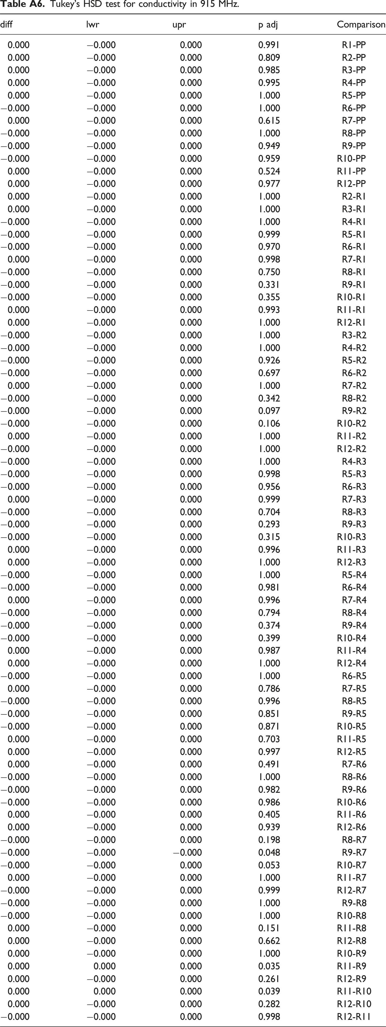

diff	lwr	upr	p adj	Comparison
0.000	−0.000	0.000	0.991	R1-PP
0.000	−0.000	0.000	0.809	R2-PP
0.000	−0.000	0.000	0.985	R3-PP
0.000	−0.000	0.000	0.995	R4-PP
0.000	−0.000	0.000	1.000	R5-PP
−0.000	−0.000	0.000	1.000	R6-PP
0.000	−0.000	0.000	0.615	R7-PP
−0.000	−0.000	0.000	1.000	R8-PP
−0.000	−0.000	0.000	0.949	R9-PP
−0.000	−0.000	0.000	0.959	R10-PP
0.000	−0.000	0.000	0.524	R11-PP
0.000	−0.000	0.000	0.977	R12-PP
0.000	−0.000	0.000	1.000	R2-R1
0.000	−0.000	0.000	1.000	R3-R1
−0.000	−0.000	0.000	1.000	R4-R1
−0.000	−0.000	0.000	0.999	R5-R1
−0.000	−0.000	0.000	0.970	R6-R1
0.000	−0.000	0.000	0.998	R7-R1
−0.000	−0.000	0.000	0.750	R8-R1
−0.000	−0.000	0.000	0.331	R9-R1
−0.000	−0.000	0.000	0.355	R10-R1
0.000	−0.000	0.000	0.993	R11-R1
0.000	−0.000	0.000	1.000	R12-R1
−0.000	−0.000	0.000	1.000	R3-R2
−0.000	−0.000	0.000	1.000	R4-R2
−0.000	−0.000	0.000	0.926	R5-R2
−0.000	−0.000	0.000	0.697	R6-R2
0.000	−0.000	0.000	1.000	R7-R2
−0.000	−0.000	0.000	0.342	R8-R2
−0.000	−0.000	0.000	0.097	R9-R2
−0.000	−0.000	0.000	0.106	R10-R2
0.000	−0.000	0.000	1.000	R11-R2
−0.000	−0.000	0.000	1.000	R12-R2
−0.000	−0.000	0.000	1.000	R4-R3
−0.000	−0.000	0.000	0.998	R5-R3
−0.000	−0.000	0.000	0.956	R6-R3
0.000	−0.000	0.000	0.999	R7-R3
−0.000	−0.000	0.000	0.704	R8-R3
−0.000	−0.000	0.000	0.293	R9-R3
−0.000	−0.000	0.000	0.315	R10-R3
0.000	−0.000	0.000	0.996	R11-R3
0.000	−0.000	0.000	1.000	R12-R3
−0.000	−0.000	0.000	1.000	R5-R4
−0.000	−0.000	0.000	0.981	R6-R4
0.000	−0.000	0.000	0.996	R7-R4
−0.000	−0.000	0.000	0.794	R8-R4
−0.000	−0.000	0.000	0.374	R9-R4
−0.000	−0.000	0.000	0.399	R10-R4
0.000	−0.000	0.000	0.987	R11-R4
0.000	−0.000	0.000	1.000	R12-R4
−0.000	−0.000	0.000	1.000	R6-R5
0.000	−0.000	0.000	0.786	R7-R5
−0.000	−0.000	0.000	0.996	R8-R5
−0.000	−0.000	0.000	0.851	R9-R5
−0.000	−0.000	0.000	0.871	R10-R5
0.000	−0.000	0.000	0.703	R11-R5
0.000	−0.000	0.000	0.997	R12-R5
0.000	−0.000	0.000	0.491	R7-R6
−0.000	−0.000	0.000	1.000	R8-R6
−0.000	−0.000	0.000	0.982	R9-R6
−0.000	−0.000	0.000	0.986	R10-R6
0.000	−0.000	0.000	0.405	R11-R6
0.000	−0.000	0.000	0.939	R12-R6
−0.000	−0.000	0.000	0.198	R8-R7
−0.000	−0.000	−0.000	0.048	R9-R7
−0.000	−0.000	0.000	0.053	R10-R7
0.000	−0.000	0.000	1.000	R11-R7
−0.000	−0.000	0.000	0.999	R12-R7
−0.000	−0.000	0.000	1.000	R9-R8
−0.000	−0.000	0.000	1.000	R10-R8
0.000	−0.000	0.000	0.151	R11-R8
0.000	−0.000	0.000	0.662	R12-R8
0.000	−0.000	0.000	1.000	R10-R9
0.000	0.000	0.000	0.035	R11-R9
0.000	−0.000	0.000	0.261	R12-R9
0.000	0.000	0.000	0.039	R11-R10
0.000	−0.000	0.000	0.282	R12-R10
−0.000	−0.000	0.000	0.998	R12-R11

References

Rydz

Sikorska

Kyulavska

, et al. Polyester-based (bio) degradable polymers as environmentally friendly materials for sustainable development. Int J Mol Sci 2014; 16: 564–596.

Aberoumand

Rahmatabadi

Aminzadeh

, et al. 4D printing by fused deposition modeling (FDM). In: Fused Deposition Modeling Based 3D Printing. Materials Forming, Machining and Tribology. Cham: Springer, 2021, pp. 377–402.

Rus

Tolley

. Design, fabrication and control of soft robots. Nat 2015; 521: 467–475.

Kumar

Bhandari

Sharma

, et al. Polymer matrix composites: a state of art review. Mater Today Proc 2022; 57: 2330–2333.

Samir

Ashour

Hakim

AAA

, et al. Recent advances in biodegradable polymers for sustainable applications. NPJ Mater Degrad 2022; 6: 68.

MacLeod

Arp

HPH

Tekman

, et al. The global threat from plastic pollution. Science 2021; 373: 61–65.

Sajan

Philip

. A review on polymer matrix composite materials and their applications. Mater Today Proc 2021; 47: 5493–5498.

Nourbakhsh

Hosseinzadeh

Basiji

. Effects of filler content and compatibilizing agents on mechanical behavior of the particle-reinforced composites. J Polym Environ 2011; 19: 908–911.

Rahmatabadi

Mirasadi

Bayati

, et al. 4D printing thermo-magneto-responsive PETG-Fe3O4 nanocomposites with enhanced shape memory effects. Appl Mater Today 2024; 40: 102361.

10.

Rahmatabadi

Bayati

Khajepour

, et al. Poly(ethylene terephthalate) glycol/carbon black composites for 4D printing. Mater Chem Phys 2024; 325: 129737.

11.

Karimi

Rahmatabadi

Baghani

. Various FDM mechanisms used in the fabrication of continuous-fiber reinforced composites: a review. Polymers 2024; 16: 831.

12.

Jubsilp

Mora

Bielawski

, et al. Thermosetting matrix based glass and carbon fiber composites. Fiber Reinf Compos Const Compat Perspect Appl 2021: 341–403.

13.

Dhiman

Guleria

Sharma

. Applications and future trends of carbon fiber reinforced polymer composites: a review. Int Res J Eng Technol 2020; 7: 1–7.

14.

Khalid

Al Rashid

Arif

, et al. Natural fiber reinforced composites: sustainable materials for emerging applications. Results Eng 2021; 11: 100263.

15.

Zwawi

A review on natural fiber bio-composites, surface modifications and applications. Mol 2021; 26: 404.

16.

Skosana

Khoathane

Malwela

. Driving towards sustainability: a review of natural fiber reinforced polymer composites for eco-friendly automotive light-weighting. J Thermoplast Compos Mater 2024; 38(1). DOI: 10.1177/08927057241254324. Epub ahead of print May 2024.

17.

Lotfi

Dao

, et al. Natural fiber–reinforced composites: a review on material, manufacturing, and machinability. J Thermoplast Compos Mater 2019; 34: 238–284.

18.

Cui

Wang

, et al. Research on moisture absorption behavior of recycled polypropylene matrix wood plastic composites. J Thermoplast Compos Mater 2010; 24: 65–82.

19.

Jiang

Wang

, et al. Significant reinforcement of polypropylene/wood flour composites by high extent of interfacial interaction. J Thermoplast Compos Mater 2018; 32: 577–592.

20.

Farshid

Safdari

Nourbakhsh

, et al. The effects of fiber length and fiber loading on the mechanical properties of wood-plastic (polypropylene) composites. Turk J Agric For 2010; 34: 191–196.

21.

Haque

Ardila-Rey

Umar

, et al. Application and suitability of polymeric materials as insulators in electrical equipment. Energies 2021; 14: 2758.

22.

Saleem

Akbar

. Review of the performance of high-voltage composite insulators. Polym 2022; 14: 431.

23.

Johansen

Rasmussen

Knudsen

. Dielectric constants and their role in plasma simulation. Fusion Multidiscip Res An Int J 2022; 3: 248–260.

24.

Huang

Liu

Zhang

, et al. All-organic polymer dielectric materials for advanced dielectric capacitors: theory, property, modified design and future prospects. Polym Rev 2023; 63: 515–573.

25.

Luo

Wang

Guo

, et al. Progress on polymer dielectrics for electrostatic capacitors application. Adv Sci 2022; 9: 2202438.

26.

Chen

Pei

Chai

, et al. Engineering the dielectric constants of polymers: from molecular to mesoscopic scales. Adv Mater 2023; 36: 2308670.

27.

Zha

Zheng

Fan

, et al. Polymer-based dielectrics with high permittivity for electric energy storage: a review. Nano Energy 2021; 89: 106438.

28.

Nazrin

Kuan

Mansour

D-EA

, et al. Innovative approaches for augmenting dielectric properties in cross-linked polyethylene (XLPE): a review. Heliyon 2024; 10: e34737.

29.

Mahtabani

Rytöluoto

Anyszka

, et al. On the silica surface modification and its effect on charge trapping and transport in PP-based dielectric nanocomposites. ACS Appl Polym Mater 2020; 2: 3148–3160.

30.

Altındal

Barkhordari

Azizian-Kalandaragh

, et al. Dielectric properties and negative-capacitance/dielectric in Au/n-Si structures with PVC and (PVC:Sm2O3) interlayer. Mater Sci Semicond Process 2022; 147: 106754.

31.

Luo

Shen

Zhou

, et al. Dielectric properties of cellulose and nanocellulose-based materials.

32.

Nayak

Reddappa

Kalagi

, et al. Electrical insulating properties of natural fibre reinforced polymer composites; a review. Int J Eng Res 2017; 6: 166–171.

33.

Khouaja

Koubaa

Ben Daly

. Dielectric properties and thermal stability of cellulose high-density polyethylene bio-based composites. Ind Crops Prod 2021; 171: 113928.

34.

Khouaja

Koubaa

Ben Daly

. Study of the dielectric and chemical properties of cellulose bio-based composites. Ind Crops Prod 2024; 214: 118493.

35.

Ben Amor

Arous

Kallel

. Effect of maleic anhydride on dielectric properties of natural fiber composite. J Electrost 2014; 72: 156–160.

36.

George

Joseph

Nagarajan

, et al. Dielectric behaviour of PP/jute yarn commingled composites: effect of fibre content, chemical treatments, temperature and moisture. Compos Part A Appl Sci Manuf 2013; 47: 12–21.

37.

Chollakup

Tantatherdtam

Ujjin

, et al. Pineapple leaf fiber reinforced thermoplastic composites: effects of fiber length and fiber content on their characteristics. J Appl Polym Sci 2011; 119: 1952–1960.

38.

Zhang

Qin

, et al. Effect of fiber length and dispersion on properties of long glass fiber reinforced thermoplastic composites based on poly(butylene terephthalate). RSC Adv 2017; 7: 15439–15454.

39.

Yao

, et al. Effect fiber length on mechanical and thermal properties of glass fiber reinforced polyphenylene sulfide composite. Epub ahead of print February 2024. DOI: 10.1177/07316844241232960.

40.

Norizan

Abdan

Salit

, et al. Physical, mechanical and thermal properties of sugar palm yarn fibre loading on reinforced unsaturated polyester composites. J Phys Sci; 28: 115.

41.

Rani

MSA

Mohammad

Sua’it

, et al. Novel approach for the utilization of ionic liquid-based cellulose derivative biosourced polymer electrolytes in safe sodium-ion batteries. Polym Bull 2021; 78: 5355–5377.

42.

Nguyen

Zavarin

Barrall

. Thermal analysis of lignocellulosic materials. J Macromol Sci Macromol Chem 1981; 20: 1–65.

43.

Nabi

Jog

. Natural fiber polymer composites: a review. Adv Polym Technol 1999; 18: 351–363.

44.

Liu

Lei

Wang

, et al. Effect of fiber type and coupling treatment on properties of high-density polyethylene/natural fiber composites. Bioresources 2013; 8: 4619–4632.

45.

Lei

, et al. Natural fiber reinforced poly(vinyl chloride) composites: effect of fiber type and impact modifier. J Polym Environ 2008; 16: 250–257.

46.

Ghanbar

Yousefzade

Hemmati

, et al. Microstructure and thermal stability of polypropylene/bagasse composite foams. J Thermoplast Compos Mater 2014; 29: 799–816.

47.

Yuan

Gotama

, et al. Wood fiber reinforced polyethylene and polypropylene composites with high modulus and impact strength. 2008; 21: 195–208.

48.

Quan

Liang

, et al. Dielectric polarization in electromagnetic wave absorption: review and perspective. J Alloys Compd 2017; 728: 1065–1075.

49.

Bonardd

Robles

Barandiaran

, et al. Biocomposites with increased dielectric constant based on chitosan and nitrile-modified cellulose nanocrystals. Carbohydr Polym 2018; 199: 20–30.

50.

Sreekumar

Saiter

Joseph

, et al. Electrical properties of short sisal fiber reinforced polyester composites fabricated by resin transfer molding. Compos Part A Appl Sci Manuf 2012; 43: 507–511.

51.

Pathania

Singh

. A review on electrical properties of fiber reinforced polymer composites. Int J Theor Appl Sci 2009; 1: 34–37.

52.

Taha

TAM

Tharwat

Ismael

. A comprehensive study of structural, thermal, and dielectric properties of melt-processed polypropylene/Ni0.9Zn0.1Fe2O4 nanocomposites. J Compos Sci 2024; 8(8): 117.

53.

Bayati

Ahmadi

Rahmatabadi

, et al. 3D printed elastomers with superior stretchability and mechanical integrity by parametric optimization of extrusion process using Taguchi Method. Mater Res Express 2025; 12: 015301.

54.

Zyane

Brouillette

Belfkira

, et al. Toward green three‐phase composites with enhanced dielectric permittivity. J Appl Polym Sci 2018; 135: 46147.

55.

Panaitescu

Notingher

Ghiurea

, et al. Properties of composite materials from polyethylene and cellulose microfibrils. J Optoelectron Adv Mater 2007; 9: 2524–2528.

56.

Markiewicz

Paukszta

Borysiak

. Acoustic and dielectric properties of polypropylene-lignocellulosic materials composites. In: Polypropylene. London: InTech, 2012, pp. 193–217.

57.

Dakin

. Conduction and polarization mechanisms and trends in dielectric. IEEE Electr Insul Mag 2006; 22: 11–28.

Sample name	Fiber length (μm)	Fiber content (%)	PP content (%)	MAAP content (%)
R1	50	5	92	3
R2	75	5	92	3
R3	100	5	92	3
R4	50	10	87	3
R5	75	10	87	3
R6	100	10	87	3
R7	50	15	82	3
R8	75	15	82	3
R9	100	15	82	3
R10	50	20	77	3
R11	75	20	77	3
R12	100	20	77	3

Sample name	Fiber length (μm)	Fiber content (%)	PP content (%)	MAAP content (%)
R1	50	5	92	3
R2	75	5	92	3
R3	100	5	92	3
R4	50	10	87	3
R5	75	10	87	3
R6	100	10	87	3
R7	50	15	82	3
R8	75	15	82	3
R9	100	15	82	3
R10	50	20	77	3
R11	75	20	77	3
R12	100	20	77	3

Influence of fiber concentration and length on the dielectric,mechanical,and thermal properties of maple wood fiber-reinforced polypropylene

Abstract

Keywords

Introduction

Materials and methods

Materials

Fiber preparation

Composite preparation

Characterization

Thermal characterization

Thermogravimetric analysis

Tensile test

Three-point bending test

Morphology Investigation

Dielectric spectroscopy

Results and discussion

Thermal properties

Effect of fiber length

Effect of fiber concentration

Thermogravimetric analysis

Effect of fiber length

Effect of fiber concentration

Mechanical properties

Dielectric properties

Effect on dielectric constant and loss factor

Effect on conductivity

Morphology

Conclusion

Footnotes

Author contributions

Declaration of conflicting interests

Funding

Ethical statement

ORCID iD

Appendix

References

Sample name	Fiber length (μm)	Fiber content (%)	PP content (%)	MAAP content (%)
R1	50	5	92	3
R2	75	5	92	3
R3	100	5	92	3
R4	50	10	87	3
R5	75	10	87	3
R6	100	10	87	3
R7	50	15	82	3
R8	75	15	82	3
R9	100	15	82	3
R10	50	20	77	3
R11	75	20	77	3
R12	100	20	77	3