Sage Journals: Discover world-class research

Abstract

This study focuses on material extrusion-based (MEX) 3D printing of PLA reinforced with milled carbon fiber composite using the fused deposition modeling technique, structured through an L₁₆ orthogonal array design. The effects of key 3D printing input parameters (print temperature, layer thickness, infill pattern, and print speed) on flexural and compressive properties were recorded, including flexural force and stress and compressive force and stress. Levenberg-Marquardt (LM) and Scaled Conjugate Gradient (SCG) algorithm was developed to predict and evaluate the accuracy of the experiment. Regression analysis showed strong correlation between predicted and actual values, with LM recoding R-squared values of 0.99,983, 0.9809, and 0.98,968 for training, validation, and testing, respectively and 0.99,446, 0.98,119, and 0.98,876 for the SCG model. Both models effectively captured the relationships between input parameters and fracture toughness, with overall R-squared values of 0.99,506 for LM and 0.98,863 for SCG, indicating robust predictive performance across all datasets.

Graphical Abstract

Keywords

Short carbon fibre thermoplastic additive manufacturing ANN bending compression

Introduction

3D printing is an additive manufacturing (AM) technique that fabricates parts with complex geometries in a layer-to-layer deposition manner.^1–4 The AM technique including inkjet (IJ),^5–7 fused filament fabrication (FFF)/ fused deposition modeling (FDM),⁸ stereolithography (SLA), direct ink writing (DIW) etc. have revolutionized many industries, including automobiles,⁹ defense,¹⁰ aerospace,¹¹ electronics^12,13 and consumer products. Among various AM techniques, the material extrusion (MEX) based 3D printing technique is widely used techniques to rapidly produce prototypes and functional parts due to its flexibility, ease of use, and economy.^14,15 MEX is a 3D printing technique in which a thermoplastic is used as a feedstock material in the form of filament. The filament is fed through the roller in the liquefier unit, where it gets liquified by the heater installed, and the liquified material is made to extrude from the printer nozzle to deposit material over the build plate.^14,15 The motion of the extrusion unit installed in the 3D printer was numerically controlled using geometric code (G-code). MEX widely uses filament made from polyethylene terephthalate glycol (PETG),^16–18 acrylonitrile butadiene styrene (ABS),^19–21 polylactic acid (PLA),^2,22 and polyamide (PA)²³ to fabricate engineering applications. However, several researches on 3D printing with these thermoplastics revealed that these filaments alone could not fabricate robust parts due to constraints of mechanical, thermal, and chemical properties. Therefore, filaments produced by mixing the thermoplastics with reinforcement such as fillers, short fiber, and continuous fiber have emerged as a possible remedy to the mentioned drawbacks.

PLA and its composite were found as an ideal material due to its ease of processing, compatibility, and biodegradability.²⁴ PLA composite filaments were reinforced with synthetic fibers,²⁵ natural fibers,²⁶ ceramics,^27,28 and metals²⁹ to fabricate high-performance 3D-printed products. However, due to selection of improper MEX input process parameter, there arises a challenge of optimizing mechanical properties of the final part. Therefore, current research must focus on identifying key printing parameters that can enhance the primary mechanical properties of PLA composites. The critical MEX process parameters include printing temperature, layer thickness, layer width, infill density, infill pattern, raster angle, print speed, and nozzle diameter. Variations in these parameters directly affect the physical and mechanical performance of the part, build time and raw material usage.³⁰ As a result, multi-objective optimization techniques have become necessary to determine the optimal MEX input parameters. These techniques involve the simultaneous optimization of multiple response objectives and aim to balance trade-offs between them. Moreover, machine learning (ML) approaches, particularly artificial neural network (ANN) algorithms, have been used to model experimental data and predict optimized responses, enhancing the flexibility of optimization processes.³¹

An ANN algorithm with two hidden layers of 150 and 250 neurons was developed to predict the surface roughness of 3D-printed samples. The comparative results showed that the ANN model with 150 neurons showed the highest prediction accuracy with an R-squared value of 0.875.³² It was also noticed that an increase in infill density enhances the surface finish of the final parts. Similarly, in another study, ANN was employed using linear regression model to predict the effect of the MEX process parameters on the tensile strength of 3D-printed PLA samples. ANN predicted that PLA samples will possess the highest tensile strength of 36.162 MPa when fabricated with FDM process parameters of 70 mm/s, 200°C, and 0.26 mm feed rate, printing temperature and layer thickness, respectively.³³ Gunes et al.³⁴ used analysis of variance (ANOVA) and ANN to evaluate, optimize and predict the effect of FDM parameters on the dimensional stability of 3D-printed PLA samples. It was observed that ANOVA showed optimized dimensional stability at a layer thickness of 200 μm, wall thickness of 3 mm, infill density of 100% and concentric infill pattern. Moreover, ANN results showed the R2 value above 95%, clearly demonstrating the accuracy of the experimentation. Similarly, another study estimated the uncertainty of FDM samples using a combination of ANN-based predictive model and finite element analysis (FEA). It was found that tensile properties were successfully modeled at 98% training accuracy.³⁵ Wai et al.³⁶ used the Takagi-Sugeno fuzzy neural network to improve the tensile strength of 3D-printed PLA samples through optimization of FDM printing parameters. The results indicated that layer thickness influenced the morphology of PLA fibers, with increased infill density which reduced the air gaps and enhanced the tensile strength. Additionally, the relative error between predicted and experimental tensile strength values ranged from 5% to 10%, suggesting that the T-S fuzzy neural network model is promising for tensile strength predictions in FDM 3D printed tests. Baghi and Mansour³⁷ developed a hybrid Genetic Algorithm-ANN (GA-ANN) model to optimize the dimensional accuracy of the 3D printed parts. The model demonstrated the highest accuracy with a mean square error of 0.0528. Another study used genetic network programming (GNP) integration with ANN to improve the shear properties of single lap composites joint 3D printed using PLA material. The results showed an acceptable margin of error with an overall R² value of 0.8471, clearly indicating reliable outcomes and satisfactory agreement.³⁸

The current study introduces a novel approach to predict the compressive and flexural properties of 3D printed PLA/carbon fiber (CF) composites using a comparative analysis of artificial neural network (ANN) models. The model performance was assessed using Levenberg-Marquardt (LM) and Scaled Conjugate Gradient (SCG) backpropagation algorithms, with the accuracy of the models evaluated based on the R-squared (R²) values. By comparing the R² values for each algorithm, this research identifies the most effective method to find the complex relationships between input MEX process parameters and the mechanical properties of the 3D-printed PLA/CF composites. The results demonstrate the reliability of these models in simulating material behavior, aiding the design and optimization of high-performance PLA/CF composites for various engineering applications. This approach will enhance the understanding of the mechanical behavior of 3D printed materials and contribute to the development of smarter, data-driven design processes in additive manufacturing.

Material

The filament composed of polylactic acid (PLA) as the matrix and high-modulus milled carbon fiber (CF) (5-10 μm in size) as the reinforcement material was procured from 3D Cubic, Surat, India. This composite filament exhibits minimal shrinkage when cooled at elevated room temperature and features a matte, dark grey finish. The filament has a density of 1.3 g/cm³, tensile strength of 45.5 MPa and diameter of 1.75 ± 0.05 mm. PLA/CF filament was chosen due to its promising combination of high mechanical strength, stiffness, and sustainability. PLA is a widely used thermoplastic in 3D printing due to its biodegradability, ease of processing, and lower environmental impact compared to other polymers. The addition of carbon fiber further improves its mechanical properties, making PLA-CF an ideal material for applications requiring enhanced structural performance. This composite material has been increasingly explored in additive manufacturing for producing functional and high-performance parts, offering a cost-effective alternative to more traditional materials.

Methodology

Design of Experiment, 3D Printing and Mechanical Testing

The flexural and compression samples of ASTM D790 and ASTM D695 were designed using computer-aided design (CAD) software (Fusion 360, Student version). After the completion of the design, the design file was converted into an STL format that was further imported to the slicing software (Simplify 3D, Version 4.1.1). The STL (Standard Tessellation Language) file provides a brief description of the designed 3D model, which was interpreted by the slicer software. Using slicer software, a set of fixed and variable 3D printing parameters were selected, and the corresponding geometric code (G-code) was generated. The generated G-code was then transferred to the material extrusion-based 3D printing machine (MEX (FFF), Maker: 3D Cubic) for sample fabrication. The level of selected 3D printing variable parameters, along with fixed parameters, were presented in Table 1. Before the start of the 3D printing process, the printer bed was heated to 70°C, and the machine was kept idle for 20 minutes to reach thermal equilibrium. After achieving the equilibrium, a layer of adhesive (Magigoo Original) was applied to the bed to ensure proper adhesion during the printing process. A comprehensive illustration of the 3D printing schematic and the process parameters is shown in Figure 1.

Table 1.

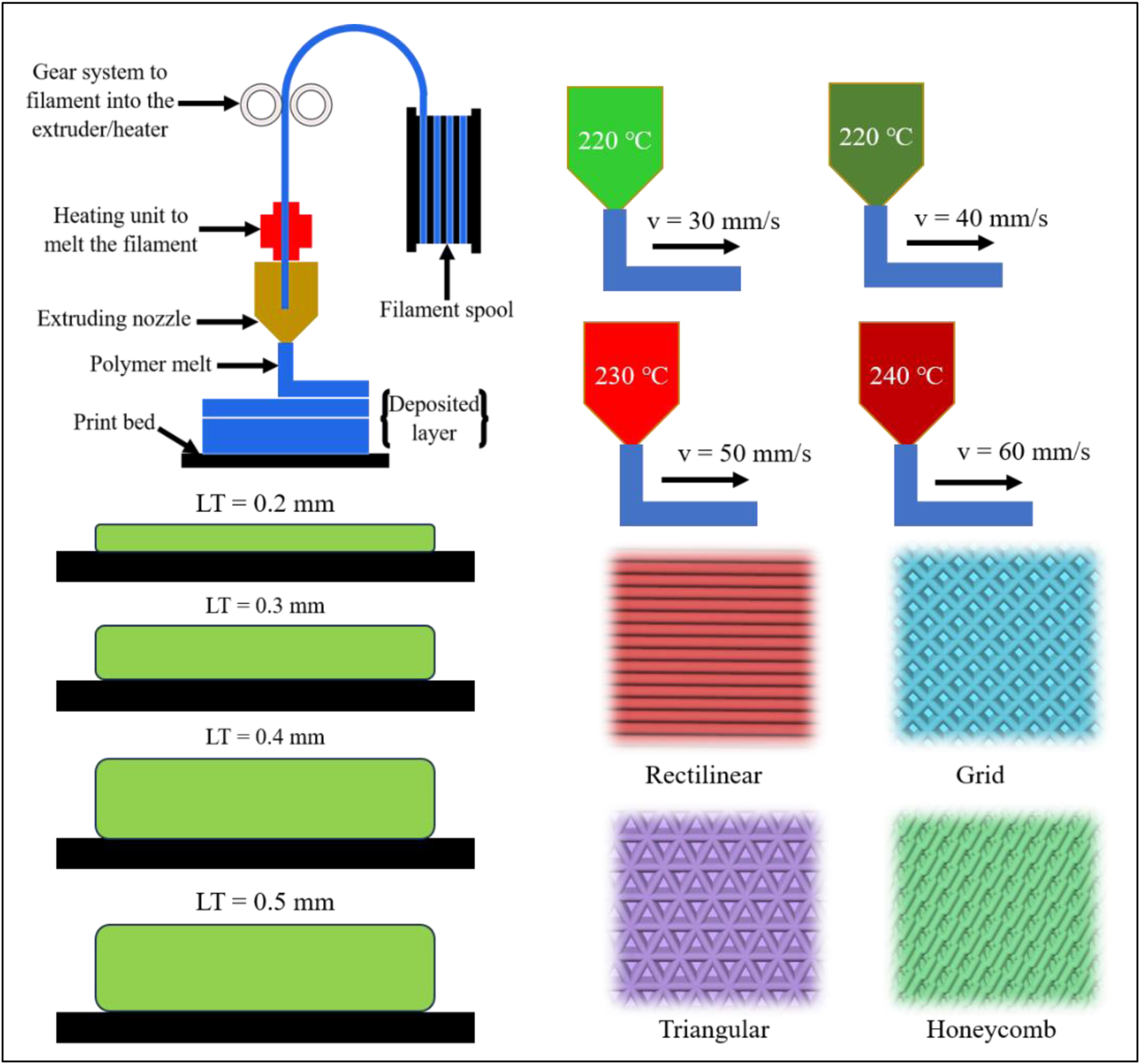
3D printing input parameters selected for the sample fabrication.

Variable		Level 1	Level 2	Level 3	Level 4	Fixed
Parameters	Units	Level 1	Level 2	Level 3	Level 4	Parameters	Units	Value
Printing temperature (PT)	°C	210	220	230	240	Bed temperature	°C	70
Layer thickness (LT)	mm	0.2	0.3	0.4	0.5	Nozzle diameter	mm	0.8
Print speed (PS)	mm/s	30	40	50	60	Build plate orientation	axis	XY
Infill pattern (IP)	-	Rectilinear (R)	Grid (G)	Triangular (T)	Honeycomb (H)	Infill ratio or density	%	100

Figure 1.

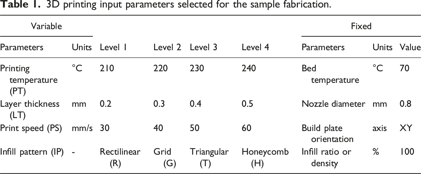
Schematic of MEX 3D printing and the process parameters used for sample fabrication.

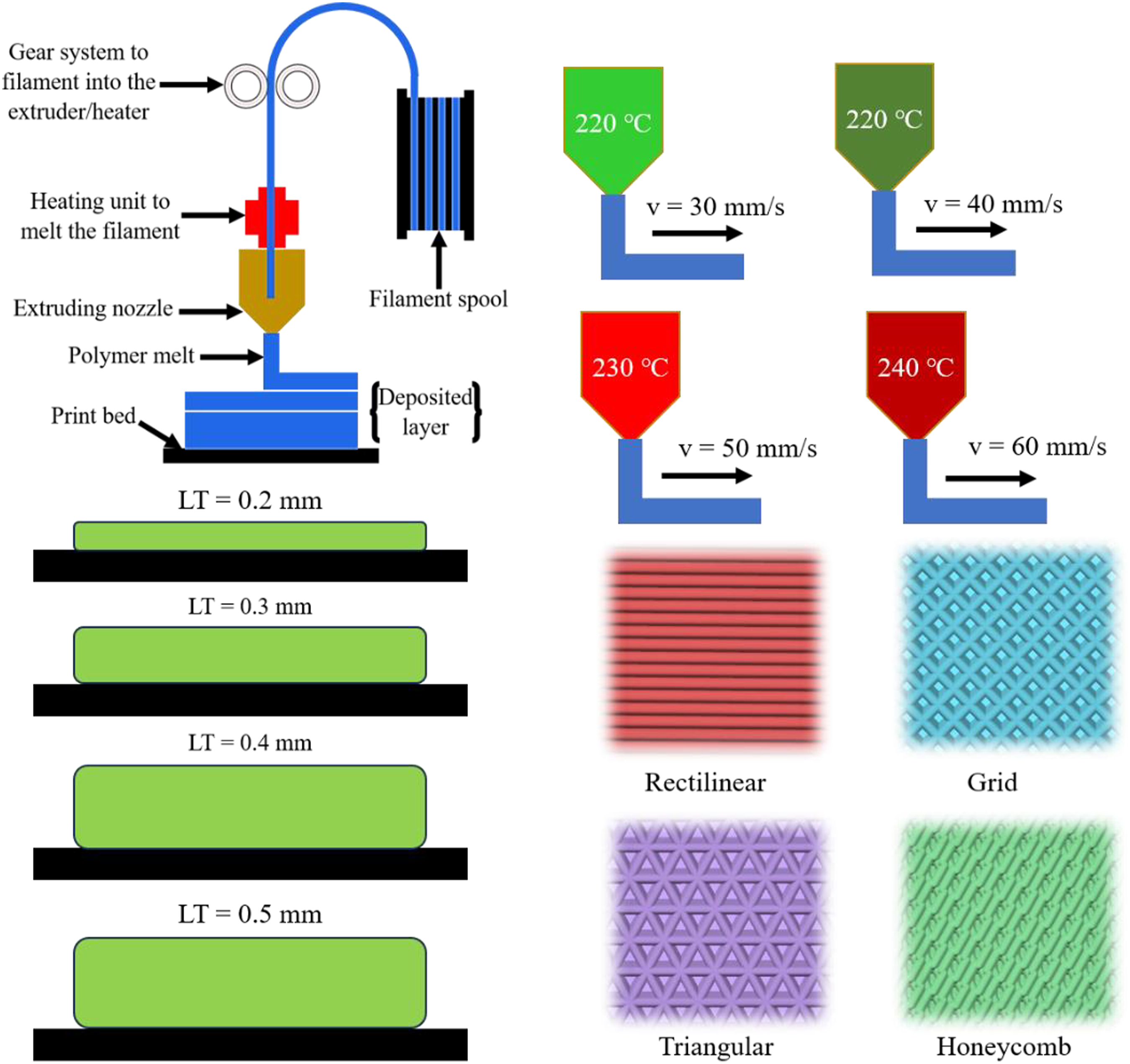
Based on the MEX input parameters, L₁₆ orthogonal array was selected to fabricate the samples. After the fabrication, flexural samples (size: 125 × 12.7 × 3.2 mm) were subjected to a three-point bend test using a 50 kN load cell universal testing machine (UTM) (Tinius Olsen, H50 KL) with a support span of 60 mm, which is 16 times the thickness of the sample. The samples were placed steadily between the end supports of the UTM fixture, and the cross-head displacement of 1 mm/min was applied through a roller for the test. Similarly, compression samples (size: 25.4 × 12.7 × 12.7 mm) were subjected to compression tests using the same UTM machine. The machine fixtures were replaced by two compression plates. The samples were sandwiched between the plates by applying 5N of load, and then the upper plate was made to compress the sample with a cross-head displacement of 1 mm/min while the bottom plate was fixed and free from any displacement. Before the tests, the sample dimensions were recorded using a vernier caliper and the room temperature was maintained at 24°C and 50% humidity. The complete illustration of the sample testing and dimension is shown in Figure 2.

Figure 2.

Flexural and compressive sample dimension with the test setup.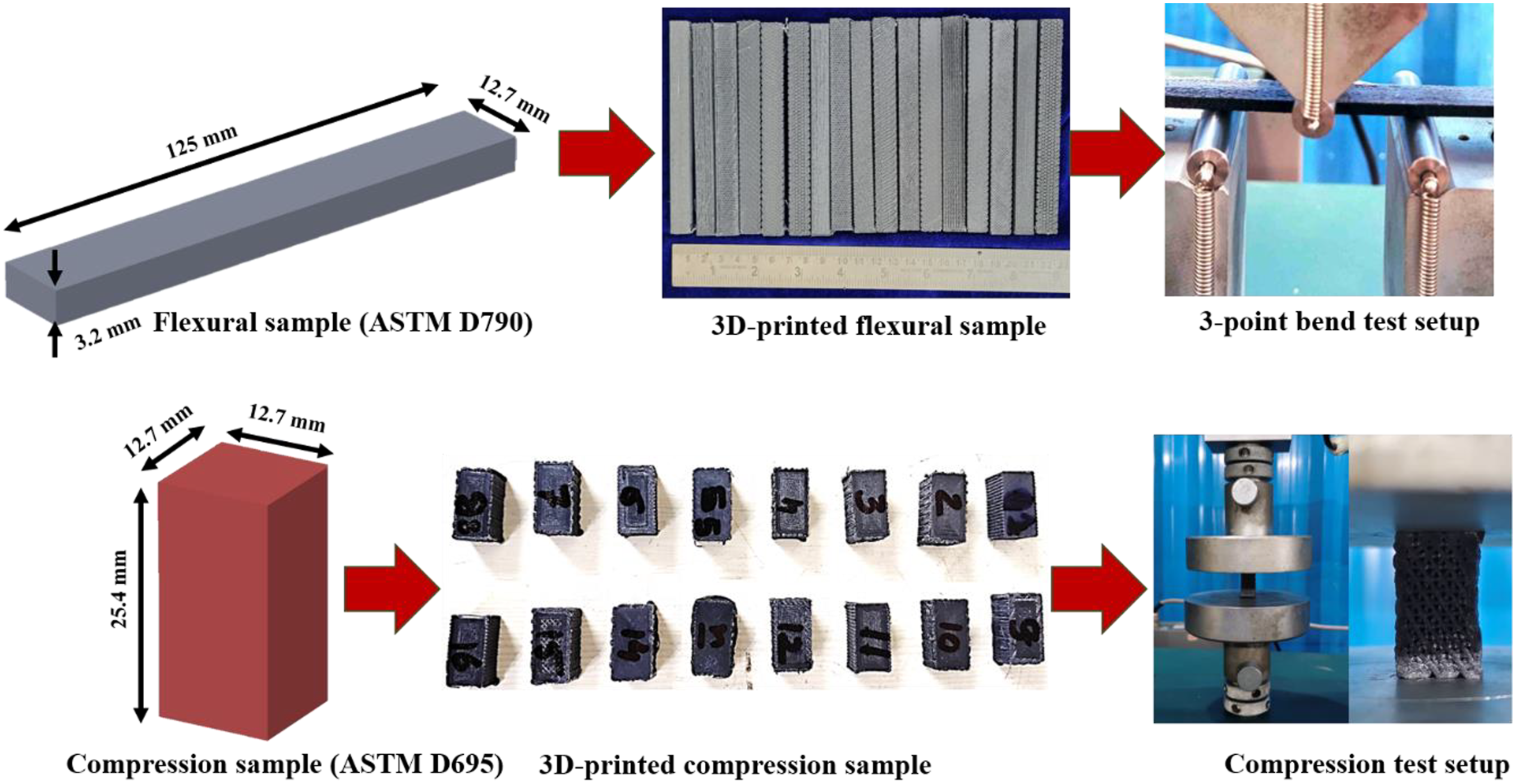

Results and Discussion

The ANN model developed in this study was trained using the Levenberg-Marquardt (LM) and Scaled Conjugate Gradient (SCG) backpropagation algorithms to estimate the relationship between inpcess parameters and output responses (i.e., compressive and flexural properties) of PLA/carbon fiber composites. The dataset was divided into 70% for training, 15% for testing, and 15% for validation. The model’s performance was assessed based solely on R-squared (R²) values, which measured the effectiveness of the ANN that evaluated the variance in the experimental data. Figure 3 presents the output responses, including maximum compressive load, compressive stress, maximum flexural load, and flexural stress, used in the analysis to determine the effectiveness of the ANN methods. Based on the DOE the numerical values of output responses are presented in Table 2.

Figure 3.

Graph illustrating (a) Compressive load and stress; (b) Flexural load and stress.

Table 2.

Output response based on design of experiments.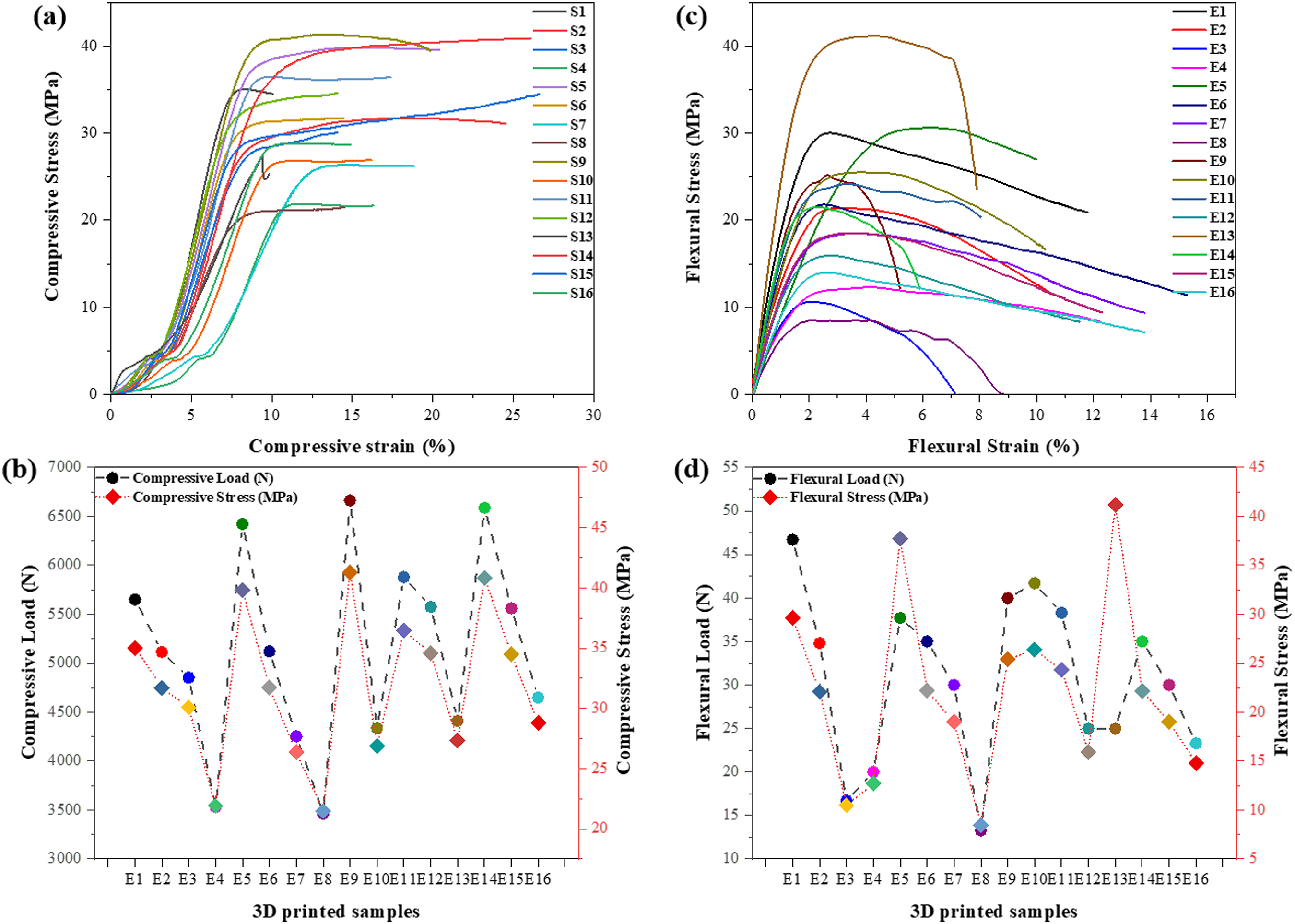

Nozzle temp	Layer thickness	Infill pattern	Print speed	Comp. Load	Comp. Stress	Flexural load	Flexural stress
°C	mm	-	mm/s	N	MPa	N	MPa
210	0.2	Rectilinear	30	5651	35.04	46.7	29.6
210	0.3	Grid	40	5115	31.71	34.8	22.1
210	0.4	Triangular	50	4853.33	30.09	16.7	10.5
210	0.5	Honeycomb	60	3531.67	21.9	20	12.7
220	0.2	Grid	50	6423.33	39.82	37.7	37.7
220	0.3	Rectilinear	60	5120	31.74	35	22.2
220	0.4	Honeycomb	30	4253.33	26.37	30	19
220	0.5	Triangular	40	3463.33	21.47	13.3	8.46
230	0.2	Triangular	60	6663.33	41.31	40	25.4
230	0.3	Honeycomb	50	4338.33	26.9	41.7	26.4
230	0.4	Rectilinear	40	5880.54	36.46	38.3	24.3
230	0.5	Grid	30	5576.67	34.58	25	15.9
240	0.2	Honeycomb	40	4411.67	27.35	25	41.2
240	0.3	Triangular	30	6590	40.86	35	22.2
240	0.4	Grid	60	5561.67	34.48	30	19
240	0.5	Rectilinear	50	4648.33	28.82	23.3	14.8

The mechanical performance of 3D-printed PLA/CF composite is strongly influenced by the combined effects of nozzle temperature, layer thickness, infill pattern, and print speed, which demonstrates the material’s interlayer adhesion, microstructural integrity, and stress distribution. Compression properties, such as compressive load and compressive stress, are notably higher at lower layer thicknesses of 0.2 mm and optimal nozzle temperatures of 230-240°C. This behavior can be attributed to improved layer fusion and reduced void content at finer layer resolutions, which enhance the composite’s ability to distribute and resist compressive forces. Also, at 230°C and a triangular infill pattern with a 0.2 mm layer thickness, the composite achieves a compressive load of 6.66 kN and compressive stress of 41.31 MPa, highlighting the collaborative effect of optimized thermal and geometric parameters. Additionally, a higher layer thickness of 5 mm result in lower compressive performance due to reduced interlayer bonding and increased surface roughness, which introduce stress concentrators.

The flexural performance of the composite also demonstrates a strong dependency on the experimental parameters. At a nozzle temperature of 240°C and a honeycomb infill pattern with a 0.2 mm layer thickness, the sample yields the highest flexural stress of 41.2 MPa. This indicates that at elevated temperatures the material might result in thermal softening, thereby improving polymer flowability, and enhancing fiber-polymer matrix bonding by interfacial adhesion. However, excessively high temperatures above 240°C can degrade the polymer matrix, leading to a decline in mechanical properties. Print speed further influences the composite’s performance. The sample fabricated at 30 mm/s print speed of 30 mm/s resulted in consistent layer deposition and greater thermal bonding, while samples 3D printed at a higher print speed of 60 mm/s caused compromised structural integrity due to incomplete fusion and uneven layer deposition. Among infill patterns, triangular and honeycomb structures perform better in terms of both compressive and flexural properties, likely due to their inherent geometric stability and stress distribution efficiency. These findings underscore the need for precise control over process parameters in FDM to optimize the mechanical behavior of PLA/Carbon fiber composites for specific load-bearing applications.

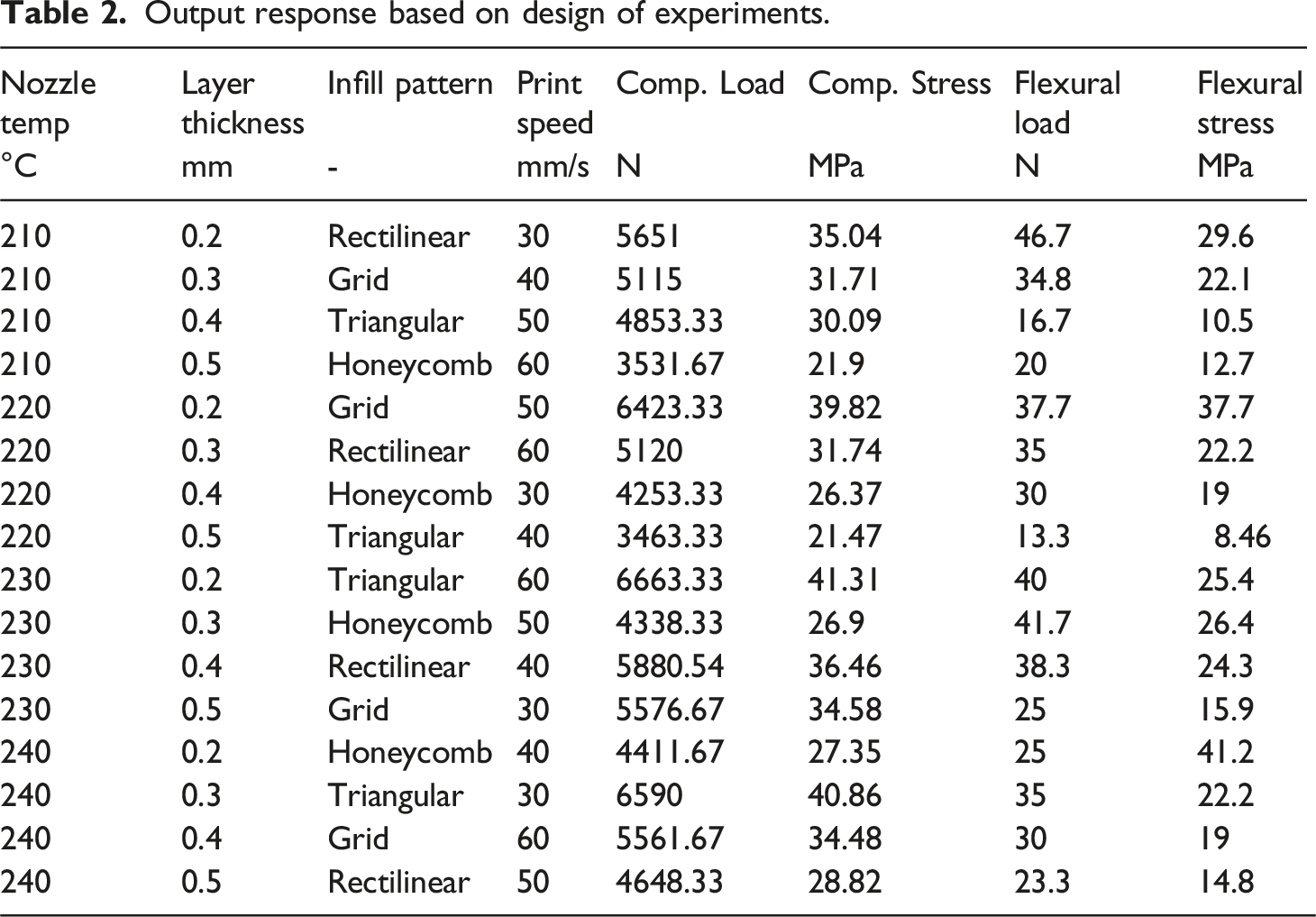
In ANN model, the dataset was split into 70% for training to enable the model to learn complex relationships between input parameters and outputs. The remaining 30% was divided evenly, with 15% allocated for testing and 15% for validation, to evaluate the model’s performance and ensure its accuracy on unseen data. This distribution helps assess the ANN’s generalization and predictive capabilities. The diagrammatic illustration of the created ANN model is shown in Figure 4. The input layer receives the input variables, which are processed through interconnected neurons in the hidden layers. Each connection, represented by lines, reflects the interaction between neurons and influences how information is transmitted and transformed. Finally, the output layer provides the model’s responses or predictions based on the learned patterns.

Figure 4.

Architecture of the Artificial Neural Network (ANN) model representing input variables, hidden layers, and output responses.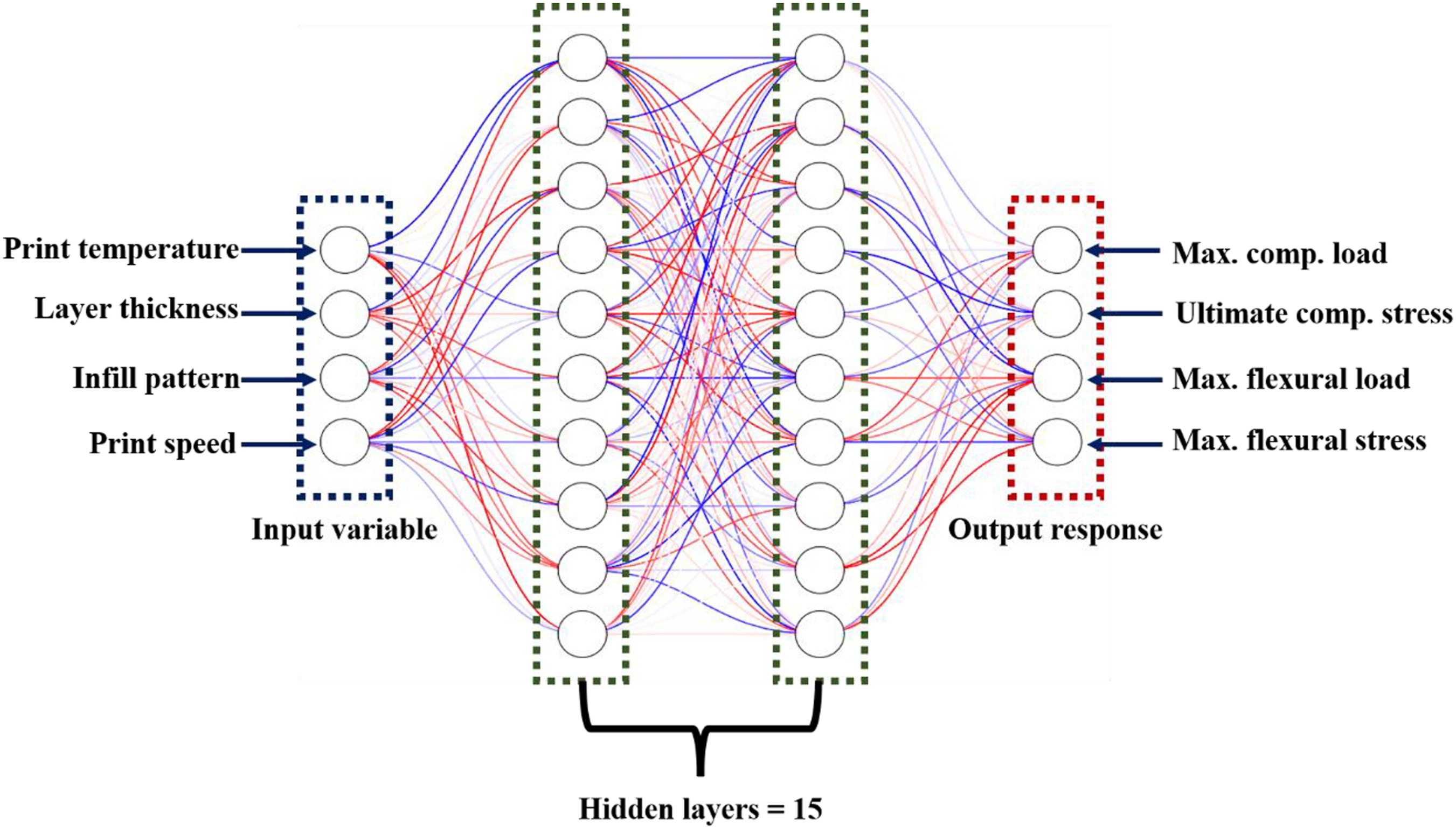

Levenberg-Marquard (LM) Algorithm

LM backpropagation ANN algorithm is an AI optimization technique that combines the advantages of gradient descent and the Gauss-Newton methods. This technique generates fast and effective solutions to minimize error functions in non-linear systems. This technique is commonly used to train ANN by adjusting the network weights that reduces the difference between actual and predicted values and improves the model accuracy. This algorithm is most suitable for problems where the dataset is small to medium-sized sized because of its relatively high computational requirements. Moreover, it adapts the dynamic learning rate, which makes it robust and less sensitive to initial parameter settings. Due to this reason, LM is regarded as an effective algorithm for achieving rapid convergence and high performance in complex networks.^39,40 Figure 5 shows the Levenberg-Marquardt backpropagation model for compression and flexural properties.

Figure 5.

Levenberg-Marquardt backpropagation model for compression and flexural properties.

Figure 5(a) shows the ANN performance during training over six iterations (epochs) which contains subplots representing gradient, Mu and validation check, respectively. Here, the gradient represents the error that was changing with respect to the weight during training. A sharp decrease in gradient is seen, which reaches a much smaller value of 8.37 × 10^−10, indicating the minimal change in error and convergence toward an optimal solution. The Mu graph plotted in the middle shows a steady decline, which dropped from 10⁻⁵ to 10⁻⁹, reflecting the transitioning of the algorithm from the steepest descent to a Gauss-Newton approach as it nears the solution. The validation check plot values reached four by the 6th epoch, illustrating that the training stopped at this point to avoid overfitting. The plots shown in Figure 5(a) confirm that the model successfully captured the relationships between the input parameters and the mechanical properties, with stable and optimized performance as demonstrated by the decreasing gradient and Mu values

Figure 5(b) shows the performance of the ANN during training, validation, and testing, using Mean Squared Error (MSE) as the performance metrics across six epochs. The best validation performance is noticed at epoch 3. After epoch 2, the validation error remains relatively flat, while the training error decreases sharply. This divergence between training and validation suggests that while the model continues to fit the training data better, it is not improving on unseen data, which is a sign of potential overfitting. The testing error line closely follows the validation error, further confirming the model’s generalization capabilities. The early stopping mechanism triggered at epoch 2 based on the validation checks, prevents the model from overfitting.

Figure 5(c) demonstrates the error histogram, displaying the error distribution (the difference between predicted and actual target values) for the training, validation, and test datasets in the ANN model. The X-axis represents the range of errors, where positive values indicate that the model’s predictions were lower than the actual values, and negative values indicate overpredictions. It is noticed that majority of errors cluster near zero, with a peak at the center, indicating that most predictions were close to the target values, suggesting that the model performed well. However, a few instances of higher errors are visible on both sides of the zero-error line, representing some outliers where the model’s predictions deviated from the actual values. These deviations may indicate cases where the model struggled to generalize for certain input combinations, although overall, the close-to-zero concentration of errors suggests reliable predictions for the majority of the data.

Figure 5(d) shows the regression plots for the training, validation, test, and overall datasets, comparing the target values (actual) with the output values (predicted), along with the corresponding R-values, which represent the correlation between the predicted and actual values. The plots display high correlation values, with R² values of 0.99,983 for training, 0.9809 for validation, and 0.98,968 for testing, indicating an excellent fit between the predicted and actual values in all cases. The overall dataset combining training, validation, and test data, has an overall R² value of 0.99,506 clearly indicating the model has strong predictive ability across the entire dataset.

Scaled Conjugate Gradient (SCG) Algorithm

The SCG algorithm is a powerful optimization technique specifically designed to train artificial neural networks (ANNs). It’s an improved version of the traditional conjugate gradient method, incorporating a scaling mechanism to enhance stability and convergence speed. Unlike other methods that require storing the entire Hessian matrix, SCG is memory-efficient, making it ideal for large-scale problems. By effectively leveraging previous gradients, the SCG algorithm iteratively moves toward the function’s minimum point. This iterative approach ensures faster convergence compared to other methods. The algorithm’s scaling mechanism is particularly beneficial when gradients vary significantly in magnitude, as it helps maintain stability throughout the optimization process. In essence, the SCG algorithm offers a superior solution for optimizing the weights of neural networks, leading to improved performance in a wide range of applications. Figure 6 shows the results of SCG derived from compression and flexural properties.

Figure 6.

Scaled Conjugate Gradient model for compression and flexural properties.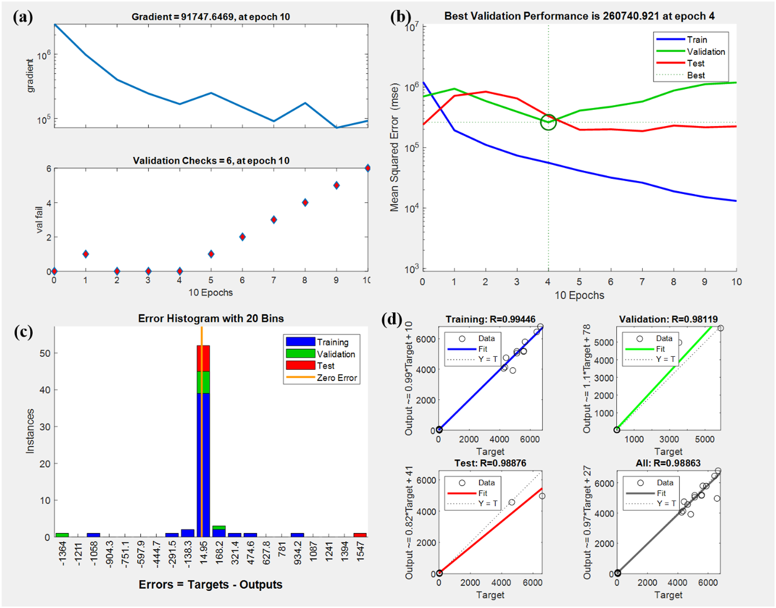

Figure 6(a) shows the training performance of an ANN using the SCG algorithm over 10 epochs. From the plot, it is noticed that the model is exhibiting signs of difficulty during training. The initial decrease in the gradient is promising, but the subsequent fluctuations suggest challenges in convergence. The steady increase in validation failures, reaching six by epoch 10, indicates overfitting. This means the model is becoming overly specialized to the training data and struggles to generalize to new, unseen data.

Figure 6(b) provided a plot depicting the mean squared error (MSE) for training, validation, and test sets over 10 epochs. The line representing the training error consistently decreases, signifying that the model is effectively learning from the training data. However, the line representing the validation error initially decreases but begins to increase after epoch 4, indicating the onset of overfitting. The line representing the test error stabilizes after epoch 4, mirroring the trend of the validation error. The best validation performance is achieved at epoch 4. This suggests that epoch 4 is the ideal stopping point for this model to prevent overfitting while maintaining strong generalization capabilities. Figure 6(c) shows the histogram representing the error distribution between the predicted and actual values. The model demonstrates strong performance, with most predictions clustering around zero error. This indicates high accuracy for the majority of data points, particularly in the training set. While a few outliers exhibit larger errors, these are infrequent. The model exhibits minimal significant deviations, suggesting satisfactory performance on the given data.

Figure 6(d) illustrates the regression plots that reveal the ANN model’s performance across training, validation, and test sets. Each plot illustrates the correlation between predicted and target values, with a linear fit line and an R² coefficient indicating the fit’s strength. The training set shows a near-perfect fit (R² = 0.99,446), while the validation set exhibits a slightly weaker correlation (R² = 0.98,119). The test set maintains a stronger correlation (R² = 0.98,876), with minor deviations in the outer points. Combining all data sets yields an excellent overall fit (R² = 0.98,863), demonstrating the model’s consistent performance.

Fracture Morphology

Figure 7 shows the failed PLA/CF compression samples indicating a range of failure models like buckling, bulging and interlayer delamination. Sample fabricated with rectilinear and grid infill patterns shown in Figure 7(a) and (k) indicates minor bulging and buckling demonstrating better stress distribution and resistance to deformation. On the other hand, the samples fabricated with honeycomb and triangular infill patterns shown in Figure 7(d) to (l), exhibited prominent buckling and bulging, especially in regions where layer adhesion was compromised due to higher layer heights and print speeds. These samples show brittle fracture characteristics, with significant interlayer separation, which suggests stress concentration leading to buckling failure. The print parameters, particularly higher print speed and thicker layers, appear to exacerbate buckling and delamination in samples shown in Figure 7(g) and (p), leading to rapid and catastrophic failure under compressive loads.

Figure 7.

Failed compression samples.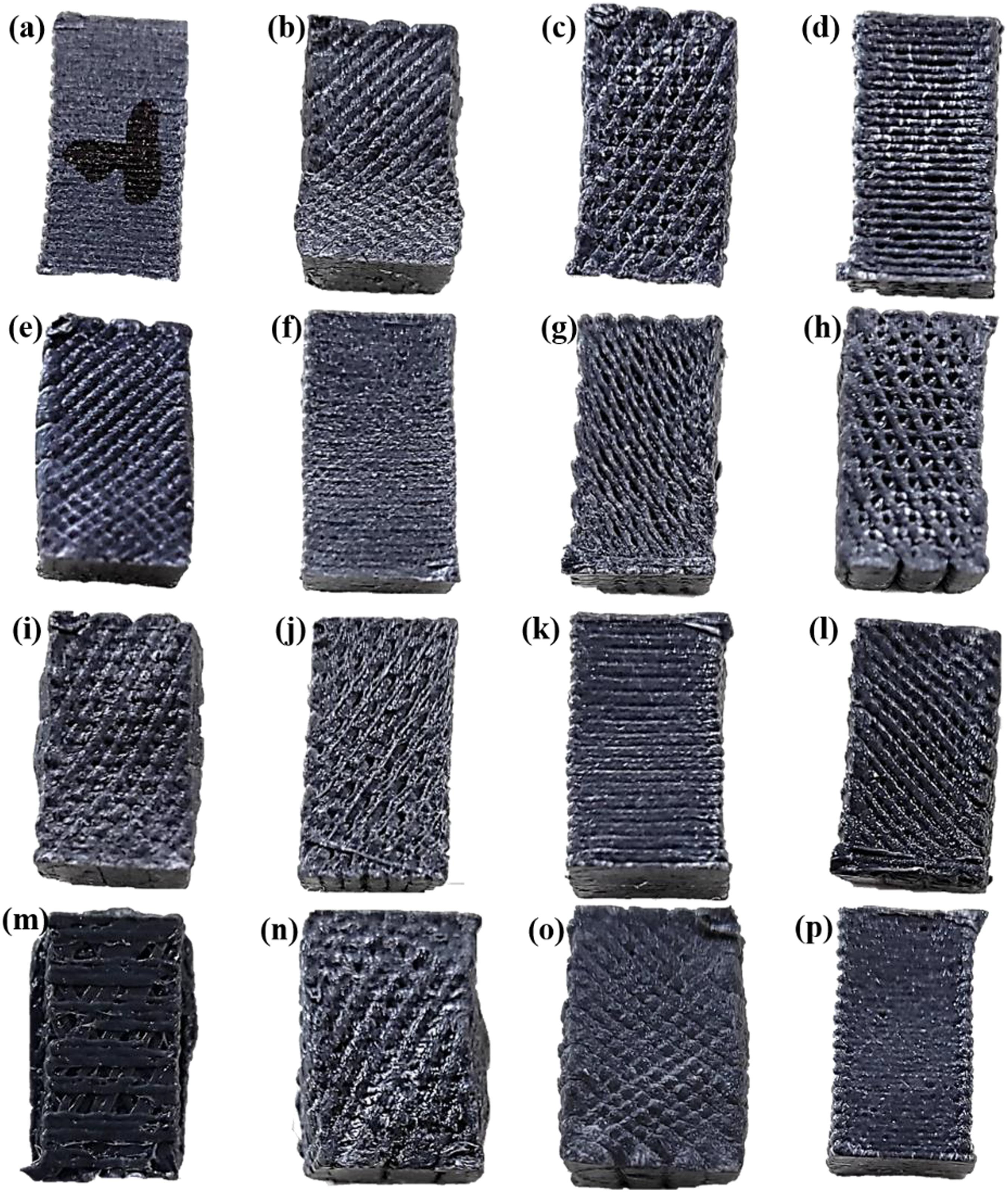

Figure 8 illustrates the fracture surfaces of CF/PLA composite samples after flexural testing, revealing distinct failure characteristics across different print conditions. Samples shown in Figure 8(a), (e) and (j) were printed with lower layer heights and rectilinear or grid infill patterns, exhibit smoother and more cohesive fracture surfaces, indicating a more gradual failure under flexural loads. In these cases, the fractures suggest better load distribution and enhanced interlayer bonding. In contrast, samples shown in Figure 8(d), (h) and (p)) were fabricated with higher layer heights and honeycomb or triangular infill patterns, shows significant delamination, fiber pull-out, and jagged fracture surfaces. These failures are characteristic of buckling and stress concentration along weak points in the layers, especially where print speed and layer height were higher, causing less adhesion between layers. Additionally, the bulging in samples shown in Figure 8(n) and eight(p) indicates excessive deformation before catastrophic failure, likely due to poor structural integrity from the selected infill patterns and print speeds. This fracture morphology highlights the critical role of infill pattern and print parameters in determining the flexural strength of 3D printed CF/PLA composites.

Figure 8.

Optical images of failure flexural samples.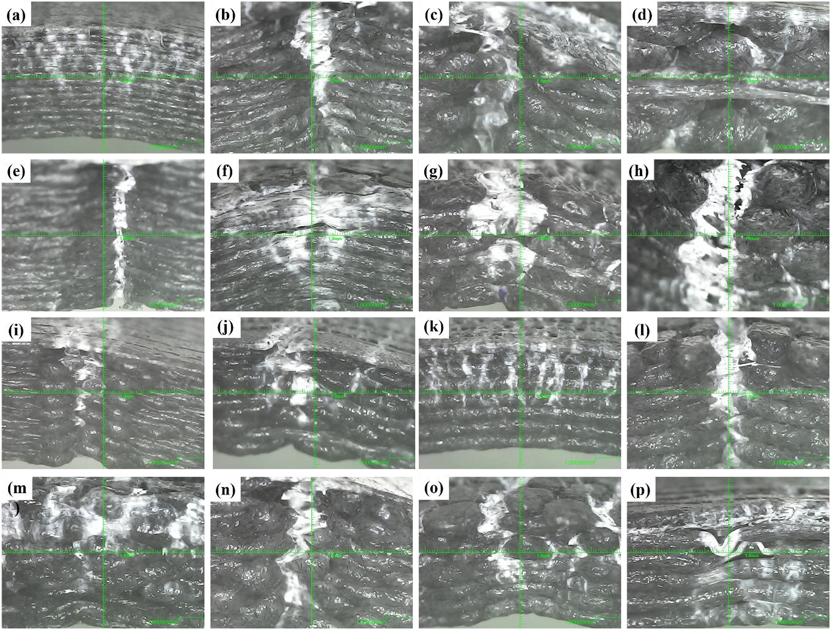

Conclusion

The current study illustrates the development of the ANN model to predict the compression and flexural properties of a 3D-printed PLA/CF sample and evaluate the model accuracy. Levenberg-Marquardt (LM) and Scaled Conjugate Gradient (SCG) algorithm was developed for the study, and the dataset was split into 70% for training and 15% for testing and validation. The LM algorithm demonstrated higher performance on small to medium datasets, achieving its best validation Mean Squared Error (MSE) at epoch 6, but showed slight overfitting as training progressed. Moreover, the SCG algorithm, which is known for its stability and suitability for large-scale problems, reached optimal performance at epoch 4. Regression analysis showed strong correlation between predicted and actual values, with LM recoding R-squared values of 0.99,983, 0.9809, and 0.98,968 for training, validation, and testing, respectively and 0.99,446, 0.98,119, and 0.98,876 for the SCG model. Both models effectively captured the relationships between input parameters and fracture toughness, with the overall R-squared values of 0.99,506 for LM and 0.98,863 for SCG, indicating robust predictive performance across all datasets.

Footnotes

Acknowledgements

The authors would like to thank Centre for Additive Manufacturing, Chennai Institute of Technology, Tamil Nadu, for providing their valuable technical support.

Declaration of conflicting interests

The author(s) declared no potential conflicts of interest with respect to the research, authorship, and/or publication of this article.

Funding

The author(s) received no financial support for the research, authorship, and/or publication of this article.

ORCID iDs

Vishal Mishra

Dhinakaran Veeman

References

Rahman

Islam

Dip

, et al. A review on nanomaterial-based additive manufacturing: dynamics in properties, prospects, and challenges. Prog Addit Manuf 2024; 9: 1197–1224. DOI: 10.1007/s40964-023-00514-8.

Wang

. Research progress in polylactic acid processing for 3D printing. J Manuf Process 2024; 1: 1.

D-S

Lalit

, et al. A hybrid FBG-based load and vibration transducer with a 3D fused deposition modelling approach. Meas Sci Technol 2022; 33: 065106. DOI: 10.1088/1361-6501/ac5a9b.

Peng

Han

Liu

, et al. Effect of manufacturing process parameters on the compression and energy absorption properties of 4D-printed deformable honeycomb structure. Smart Mater Struct 2024; 33: 075035. DOI: 10.1088/1361-665X/ad56e7.

Chiu

. Error diffusion based feedforward height control for inkjet 3D printing. In: 2023 IEEE/ASME international conference on advanced intelligent mechatronics (AIM), 2023. DOI: 10.1109/AIM46323.2023.10196116.

Chiu

. An improved model of height profile for drop-on-demand print of ultraviolet curable ink. ASME Lett Dyn Syst Control 2021; 1: 1. DOI: 10.1115/1.4050012.

Chiu

. Modeling height profile for drop-on-demand print of UV curable ink. In: ASME 2019 dynamic systems and control conference, 2019. DOI: 10.1115/DSCC2019-9242.

Kumar

. Mechanical, morphological, and dimensional properties of heat-treated fused deposition modeling printed polymeric matrix of polyethylene terephthalate glycol. In: Progress in rubber, plastics and recycling Technology, 2023. DOI: 10.1177/14777606231218354.

RSM . Parametric optimization of fused deposition modelling process using Grey based Taguchi and TOPSIS methods for an automotive component. Rapid Prototyp J 2021; 1: 2. DOI: 10.1108/RPJ-10-2019-0269.

10.

Marciniak

. The 3D printing in military applications: FDM Technology, materials, and implications. AiMT 2023; 18: 241–257. DOI: 10.3849/aimt.01846.

11.

Brischetto

. A multipurpose modular drone with adjustable arms produced via the FDM additive manufacturing process. In: Curved and layered structures, 2016.

12.

Singh

Kumar

Chohan

, et al. Investigation of copper reinforced Acrylonitrile Butadiene Styrene and Nylon 6 based thermoplastic polymer nanocomposite filaments for 3D printing of electronic components. High Perform Polym 2022; 35: 115–125. DOI: 10.1177/09540083221112307.

13.

Kumar

Duvedi

Sharma

, et al. Navigating the frontier: additive Manufacturing’s role in synthesizing piezoelectric materials for flexible electronics. J Thermoplast Compos Mater 2024. DOI: 10.1177/08927057241270729.

14.

Mishra

Negi

Kar

, et al. Recent advances in fused deposition modeling based additive manufacturing of thermoplastic composite structures: a review. J Thermoplast Compos Mater 2022; 36: 3094–3132. DOI: 10.1177/08927057221102857.

15.

Mishra

Negi

Kar

. FDM-based additive manufacturing of recycled thermoplastics and associated composites. J Mater Cycles Waste Manag 2023; 25: 758–784. DOI: 10.1007/s10163-022-01588-2.

16.

Kumaresan

Samykano

Kadirgama

, et al. Effects of printing parameters on the mechanical characteristics and mathematical modeling of FDM-printed PETG. Int J Adv Manuf Technol 2023; 128: 3471–3489. DOI: 10.1007/s00170-023-12155-w.

17.

Erdaş

. Experimental analysis of the effects of different production directions on the mechanical characteristics of ABS, PLA, and PETG materials produced by FDM. Mater Test 2024; 1: 2.

18.

Iacob

Zisopol

Minescu

. Technical-economical study on the optimization of FDM parameters for the manufacture of PETG and ASA parts. Polymers 2024; 16: 2260. DOI: 10.3390/polym16162260.

19.

Tran

Deng

Canturri

, et al. Highly-dense acrylonitrile butadiene styrene specimens fabricated by overheat material extrusion 3D printing. Rapid Prototyp J 2023; 29: 687–696. DOI: 10.1108/RPJ-06-2022-0184.

20.

Wang

. Effects of FDM-3D printing parameters on mechanical properties and microstructure of CF/PEEK and GF/PEEK. Chin J Aeronaut 2021; 1: 2.

21.

Zha

Zhang

. Reversible negative compressibility metamaterials inspired by Braess’s Paradox. Smart Mater Struct 2024; 33: 075036. DOI: 10.1088/1361-665X/ad59e6.

22.

Joseph

Kallingal

Suresh

, et al. 3D printing of polylactic acid: recent advances and opportunities. Int J Adv Manuf Technol 2023; 125: 1015–1035. DOI: 10.1007/s00170-022-10795-y.

23.

Yilmaz

. Comprehensive analysis of 3D printed PA6.6 and fiber-reinforced variants: revealing mechanical properties and adhesive wear behavior. Polym Compos 2024; 1: 2.

24.

Kumar

Singh

Kumar

, et al. Mechanical and morphological characterizations of laminated object manufactured 3D printed biodegradable poly(lactic)acid with various physical configurations. J Mar Sci Eng 2022; 10: 1954. DOI: 10.3390/jmse10121954.

25.

Vălean

, et al. Static and fatigue behavior of 3D printed smooth and notched PLA and short carbon fibers reinforced PLA. Theor Appl Fract Mech 2024; 1: 1.

26.

Benabderazag

, et al. Characterization of thermomechanical properties and damage mechanisms using acoustic emission of Lygeum spartum PLA 3D-printed biocomposite with fused deposition modelling. Compos Appl Sci Manuf 2024; 1: 1.

27.

Mushtaq Alam

, et al. Fabrication, mechanical, finite element and in vitro evaluation of 3D printed polylactide/biphasic calcium phosphate composite blends. Mater Chem Phys 2024; 1: 1.

28.

Kumar

Singh

, et al. Multi material 3D printing of PLA-PA6/TiO2 polymeric matrix: flexural, wear and morphological properties. J Thermoplast Compos Mater 2020; 35: 2105–2124. DOI: 10.1177/0892705720953193.

29.

Hasanzadeh

. Process-property relationship in polylactic acid composites reinforced by iron microparticles and 3D printed by fused filament fabrication. Polym Eng Sci 2024; 2: 2.

30.

Mishra

Kumar

Bhatt

, et al. Parametric optimisation of 3D-printed PLA/wood dust composite for load-bearing application using grey relational analysis. Proc IME E J Process Mech Eng 2024; 3: 1. DOI: 10.1177/09544089241241460.

31.

Castro

. Prediction of compressive strength in additively fabricated part using long short term memory based neural network. Mater Today Commun 2023; 1: 2.

32.

Chinchanikar

. ANN modelling of surface roughness of FDM parts considering the effect of hidden layers, neurons, and process parameters. In: Advances in materials and processing technologies, 2024. DOI: 10.1080/2374068X.2022.2091085.

33.

Hamouti

El Farissi

Laouardi

. Experimental study of the effect of different 3D printing parameters on tensile strength, using artificial neural network. Mater Res Express 2024; 11: 035505. DOI: 10.1088/2053-1591/ad3465.

34.

Gunes

. Application of artificial neural network to evaluation of dimensional accuracy of 3D-printed polylactic acid parts. J Polym Sci 2024; 3: 8.

35.

Obaidat

Tamimi

Mumani

, et al. An artificial neural network-based predictive model for tensile behavior estimation under uncertainty for fused deposition modeling. Rapid Prototyp J 2024; 30: 2056–2070. DOI: 10.1108/RPJ-04-2024-0168.

36.

Wei

. Optimizing FDM 3D printing parameters for improved tensile strength using the Takagi–Sugeno fuzzy neural network. Mater Today Commun 2024; 0: 1.

37.

Hashemi Baghi

Mansour

. Development of a genetic algorithm – artificial neural network model to optimize the dimensional accuracy of parts printed by FFF. Rapid Prototyp J 2024; 30: 840–857. DOI: 10.1108/RPJ-09-2023-0314.

38.

Anand

Satyarthi

. Neural network-based modeling of FFF process for PET-G: evaluating MLPNN and RBFNN performance in mechanical property prediction. Proc IME E J Process Mech Eng 2024; 44: 8. DOI: 10.1177/09544089241272752.

39.

Fan

Pan

. A note on the Levenberg–Marquardt parameter. Appl Math Comput 2009; 5: 4.

40.

Yan

Zhong

Lin

, et al. Adaptive levenberg–marquardt algorithm: a new optimization strategy for levenberg–marquardt neural networks. Mathematics 2021; 9: 2176. DOI: 10.3390/math9172176.

Artificial neural network-based predictive models for analyzing the flexural and compressive strength of PLA/carbon parts fabricated via material extrusion-based 3D printing

Abstract

Keywords

Introduction

Material

Methodology

Design of Experiment, 3D Printing and Mechanical Testing

Results and Discussion

Levenberg-Marquard (LM) Algorithm

Scaled Conjugate Gradient (SCG) Algorithm

Fracture Morphology

Conclusion

Footnotes

Acknowledgements

Declaration of conflicting interests

Funding

ORCID iDs

References