Sage Journals: Discover world-class research

Abstract

Fiber length is one of the vital factors in determining the properties of long fiber reinforced thermoplastics (LFRT). However, many factors may generate fiber breakage in the injection molding process of LFRT, such as friction, melt shear, injection rate, etc. Especially for thin-walled products, owing to the relatively narrow mold cavity and frozen layer near the mold wall, it’s usually difficult for the fibers to move freely with the melt, leading to fiber breakage under the shear stress of the flow field eventually. In such a situation, the existing buckling breakage model based on the assumption fibers immersed in the flow field being in an unconstrained state is no longer applicable. In this paper, a new model for calculating the critical length of constrained fiber in thin-walled injection molded products is developed. A typical long glass fiber reinforced polypropylene thin-walled product was employed to verify the reliability of the model. The high-precision fiber length analyzer was used to calculate the fiber length distribution at different distances from the injection port. At the same time, the length distribution at the corresponding position was predicted via the model. The average prediction accuracy in the three sampling sections is 87.8%, 91.4% and 83.6%, respectively. The results show that the proposed model can effectively predict the fiber length distribution of injection molded thin-walled products. This conclusion provides important support for further accurate calculation of the mechanical properties of products.

Keywords

Fiber breakage critical length thin-walled part injection molding thermoplastic composites

Introduction

Long fiber reinforced thermoplastics (LFRT) originating in the 20th century are regarded as a transitional product between short fiber reinforced thermoplastics (SFRT) and continuous fiber reinforced thermoplastics. Compared with SFRT, LFRT has better strength, stiffness, toughness and durability, and still maintains the ability to manufacture three-dimensional (3D) complex products by injection molding. Therefore, LFRT is widely used in aerospace, automobile manufacturing, sports, leisure equipment and other fields, with automotive and transport having the highest demand.^1–7

Fiber length is one of the most important factors affecting the performance of LFRT. In general, with the increase of fiber length, within a certain range, the impact strength, tensile strength, maximum yield strength, elastic modulus, crack resistance and other properties of the product have been enhanced.^8–12 However, during the LFRT injection molding process, a large number of fibers may be broken or damaged due to friction and melt shear force.^13–15 Therefore, how to optimize the mold design and process parameters to make the fiber length as long as possible in the products is particularly important. Many experimental studies show that the lower screw speed, lower back pressure and higher injection temperature are beneficial to reduce fiber breakage and improve the mechanical properties of the products.^16–19 Although the works above mentioned have indeed provided a great help in solving the problem of fiber damage, the time and economic costs are large. Fortunately, numerical simulation methods can compensate for these shortcomings. Breaux et al.²⁰ proposed two different fracture mechanisms for fiber damage at different stages of a single screw. One is for the plasticizing stage, the fiber distribution is typically bimodal type. The other is based on the fiber bonding sphere model for the complete melting stage. Durinzd et al.²¹ predicted the distribution of fiber length in the twin-screw extrusion based on a material method. Berzin et al.²² also simulated the size change of fibers at the same stage through the Ludovic^@ software. Two different distribution functions were put forward for the long tail attenuation distribution of the fiber, which was difficult to capture by the Weibull model.^23,24 Ganesh et al.²⁵ developed a bimodal Weibull model by employing two distinct experimental techniques: the single fiber tensile test and the single fiber fragmentation test. This model provides an accurate prediction of fiber strength distribution across a length range of 500 μm (0.5 mm) to 30 mm. Sasayama et al.²⁶ simulated the simple shear flow field based on the beaded chain model and found that the fiber length degraded with the increase of viscosity, shear rate and fiber volume fraction during processing. Kang et al.²⁷ established a mechanical model to characterize the effects of shear stress on fiber buckling and fracture degree on the assumption that fibers are not constrained in the injection molding shear flow field. Simacek et al.²⁸ developed a model to describe the motion and deformation of flexible elastic fibers under low Reynolds number conditions. The model specifically addresses the gradual, buckling-like folding that occurs when fibers are misaligned with the flow direction. It effectively estimates the forces exerted by the fluid on the fibers, offering insights into the complex interactions between the flow field and fiber deformation. Ganesh et al.²⁹ developed a novel continuous bending test to directly map the size and spatial distribution of surface defects on glass fibers. This method allows for the prediction of fiber failure and composite strength distribution by analyzing the distribution of defect sizes and spacings on the fiber surface.

As a matter of practical injection molding, the factors leading to fiber damage in the mold cavity are usually much more complex than those considered in the above-mentioned model. Especially for thin-walled products, the high-temperature melt is rapidly cooled to form a frozen layer when it comes into contact with the low-temperature mold, usually makes fibers more susceptible to being constrained by the solidified layer in the narrow cavity, resulting in the inability to move freely with the melt. As the frozen layer becomes thicker, fibers are more prone to entanglement and damage under shear stress. In such instances, fiber fracture typically occurs in a constrained state, rendering the unconstrained fiber buckling fracture model described above inapplicable.

In the present work, a new model is developed to predict the critical fracture length of restrained fibers for injection molded thin-walled products. This critical length can be used to easily determine the breakage of fiber in its current state. A typical thin-walled injection molded rectangular product of long glass fiber reinforced polypropylene was employed to verify the reliability of the model. A series of samples were taken at different positions of the product by wire saw and calcined in a muffle furnace to separate the fibers from the matrix. The length distribution of separated fibers was counted via the high-precision fiber length analyzer (FASEP 3E-ECO). Further, by using this model, the residual fiber length distribution of the products is predicted based on the temperature field, velocity field and shear field data simulated by Moldflow. The predicted results of fiber length distribution at the corresponding positions agree well with the experimental data. This indicates that the model has good reliability in predicting the fiber length of thin-walled products.

Calculation model of fiber breakage

Disturbance of fibers to the flowing melt

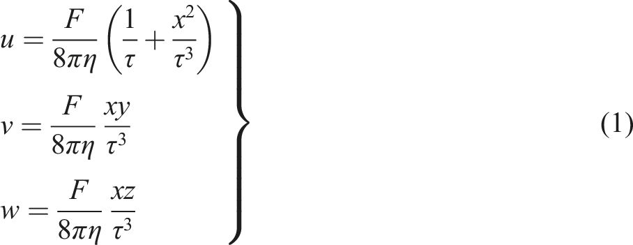
In the injection filling process of LFRT, the introduction of solid fibers will inevitably produce disturbances to the melt flow. OSEEN has provided a method for calculating the disturbance velocity of the cylindrical particles on the flow field.³⁰ As shown in Figure 1, the fiber with a length of L = 2a and a radius of b is immersed in the flow field with a velocity of V. The center of one end of the fiber is taken as the origin to establish the x, y, x coordinate system. The initial velocity V is assumed to be uniform, constant and simultaneously parallel to the x axis. According to the method proposed by OSEEN, the disturbance velocity of the fiber to the flow field can be obtained as

\begin{array}{l} u = \frac{F}{8 π η} (\frac{1}{τ} + \frac{x^{2}}{τ^{3}}) \\ v = \frac{F}{8 π η} \frac{x y}{τ^{3}} \\ w = \frac{F}{8 π η} \frac{x z}{τ^{3}} \end{array}}

(1)

where u, v, and w are the velocity components in the x, y, and z directions, respectively. F is the resistance of the fiber to the melt, which is perpendicular to its axis. η is the viscosity of the melt,

τ = x^{2} + y^{2} + z^{2}

Figure 1.

The fiber immersed in the flow field with a velocity of V.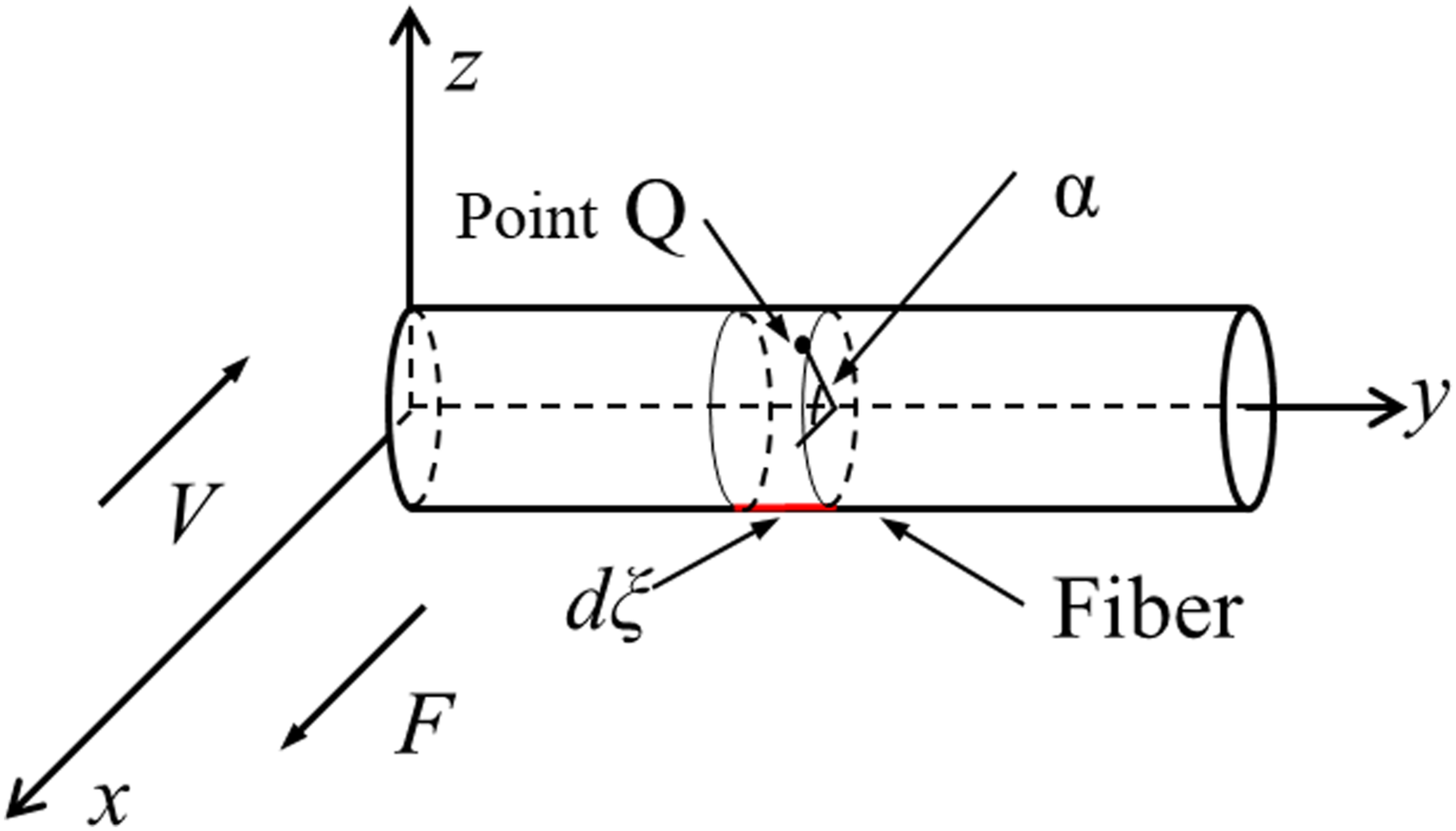

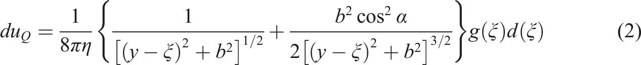
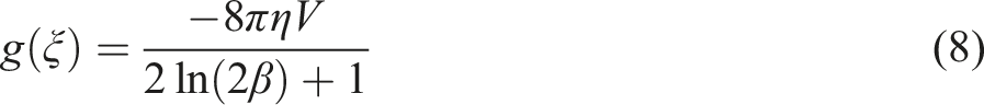
For any microelement dξ on the fiber axis, supposing the force acting on the flow field by dξ is defined as g(ξ)dξ. Q is any point on the surface of the microelement and its coordinates are x = b cosα, y = y and z = b sinα, then the disturbance velocity in x direction produced by g(ξ)dξ at Q can be expressed as

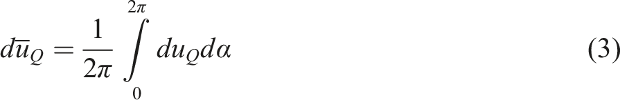
d u_{Q} = \frac{1}{8 π η} {\frac{1}{{[{(y - ξ)}^{2} + b^{2}]}^{1 / 2}} + \frac{b^{2} \cos^{2} α}{2 {[{(y - ξ)}^{2} + b^{2}]}^{3 / 2}}} g (ξ) d (ξ)

(2)

By integrating formula (2) from α = 0 to α = 2π, the average value of u over the circumference of the fiber section perpendicular to the axis can be obtained

d {\bar{u}}_{Q} = \frac{1}{2 π} \int_{0}^{2 π} d u_{Q} d α

(3)

If the formula (3) is continued to integrate for dξ from ξ = 0 to ξ = 2a, the total disturbance velocity u_Q at Q can be obtained. Assuming that there shall be no slipping of the melt along this fiber surface, then the resultant velocity of V + u_Q on the surface will be equal to zero, the following formula was obtained

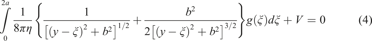
\int_{0}^{2 a} \frac{1}{8 π η} {\frac{1}{{[{(y - ξ)}^{2} + b^{2}]}^{1 / 2}} + \frac{b^{2}}{2 {[{(y - ξ)}^{2} + b^{2}]}^{3 / 2}}} g (ξ) d ξ + V = 0

(4)

Considering that the fiber is a cylinder of equal diameter, g(ξ) can be approximately regarded as a constant in the axial direction and taken as the value of the central section (y = a) of the fiber. Based on this, we can implement the integration of equation (4). Assuming that (y-ξ) = h and dξ = -dh, then equation (4) can be transformed into

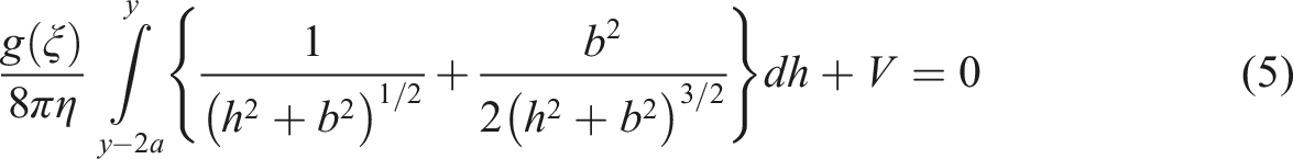
\frac{g (ξ)}{8 π η} \int_{y - 2 a}^{y} {\frac{1}{{(h^{2} + b^{2})}^{1 / 2}} + \frac{b^{2}}{2 {(h^{2} + b^{2})}^{3 / 2}}} d h + V = 0

(5)

Integral equation (5), then there is

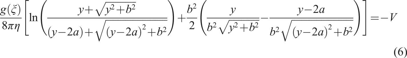
\frac{g (ξ)}{8 π η} [\ln (\frac{y + \sqrt{y^{2} + b^{2}}}{(y - 2 a) + \sqrt{{(y - 2 a)}^{2} + b^{2}}}) + \frac{b^{2}}{2} (\frac{y}{b^{2} \sqrt{y^{2} + b^{2}}} - \frac{y - 2 a}{b^{2} \sqrt{{(y - 2 a)}^{2} + b^{2}}})] = - V

(6)

Let y = a, thus

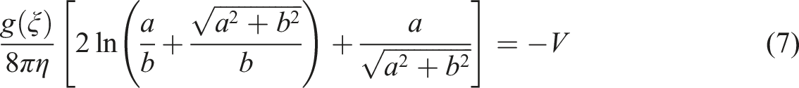
\frac{g (ξ)}{8 π η} [2 \ln (\frac{a}{b} + \frac{\sqrt{a^{2} + b^{2}}}{b}) + \frac{a}{\sqrt{a^{2} + b^{2}}}] = - V

(7)

Due to large aspect ratio of fiber, the terms of the order b²/a² in equation (7) can be further neglected, therefore g(ξ) can be expressed as

g (ξ) = \frac{- 8 π η V}{2 \ln (2 β) + 1}

(8)

where β = a/b is aspect ratio of fiber. Since the disturbance velocity v and w are symmetrical with respect to y and z, respectively, their mean value will automatically be zero at any cross section of the fiber. Therefore, it is sufficient to calculate the disturbance of fibers to the flowing melt only in the x direction.

Force exerted on the fiber in injection molding

For the molding of thin-walled products, most of the long fibers cannot move freely with the melt due to the narrow cavity, frozen layer and their mutual entanglement. Therefore, one portion of the fibers is subjected to the force exerted by the flow field, while the other portion is constrained due to the above-mentioned factors. The forces applied to the fibers can be divided into axial and radial forces. However, the deformation or fracture of the fiber is contingent upon the radial forces, as depicted in Figure 2. Hence, in order to predict the fiber fracture length, it is essential to establish a mechanical model of fiber radial force in the injection flow field.

Figure 2.

Fibers in the cavity during injection molding.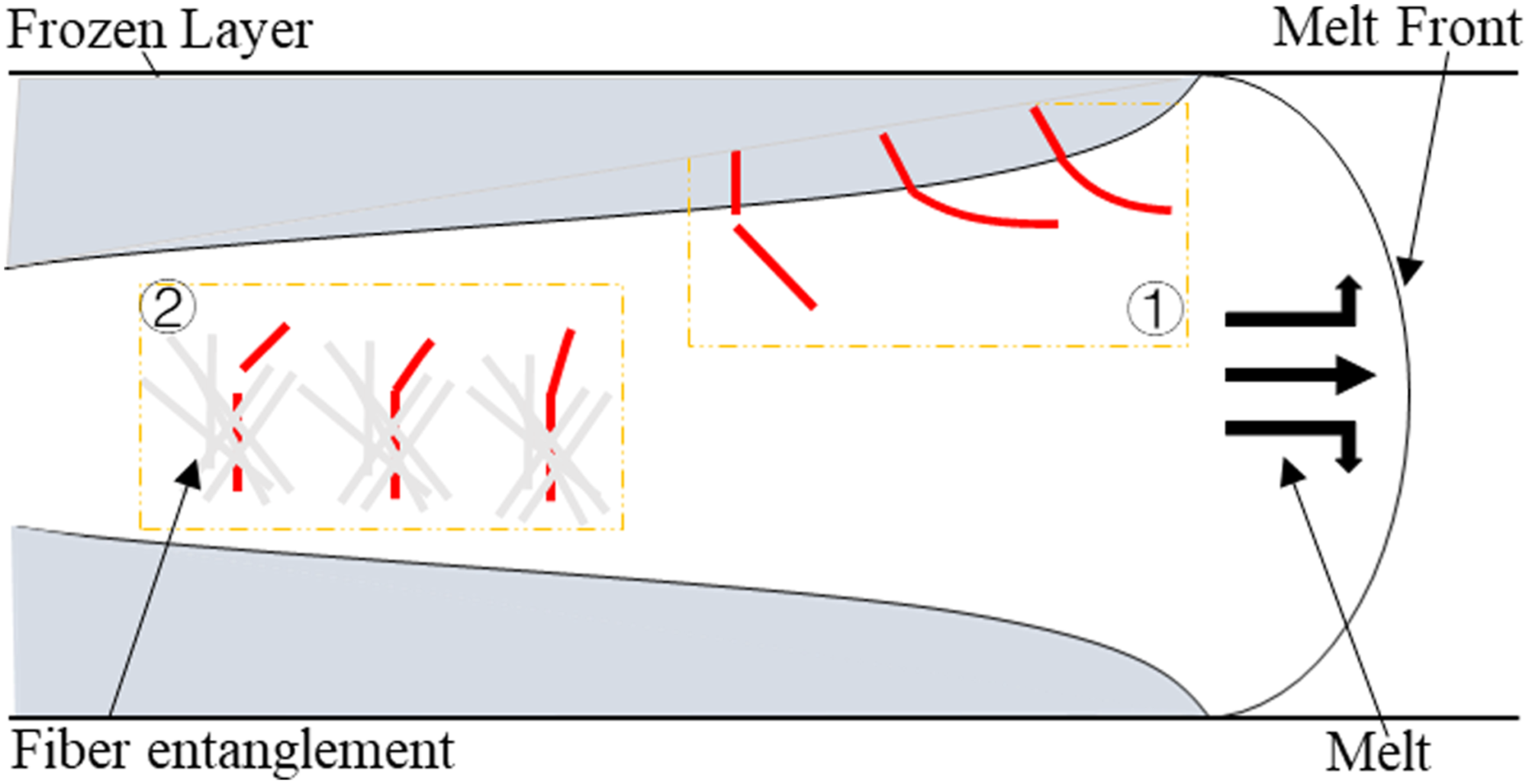

The melt flow in the filling stage of injection molding can usually be regarded as laminar flow because of the melt high viscosity. Moreover, it is a typical shear flow in the thickness direction of the mold cavity. If the flow direction of the melt is defined as the x direction, the shear flow field can be expressed as

u = \dot{γ} y, v = 0, w = 0

(9)

where

\dot{γ}

is the shear rate. The fiber immersed in the flow field is approximately described as a rigid cylinder, denoted by the unit vector P . The constrained end is taken as the origin to establish the three-dimensional coordinate system, as shown in Figure 3.

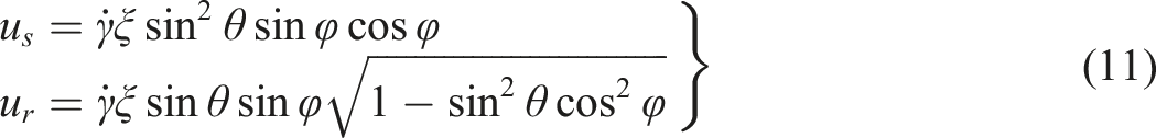
where θ refers to the included angle between fiber and z-axis, while φ refers to the included angle between the projection of fiber on the x-y plane and x-axis. It is clearly that the fiber in the flow field can be penetrate to different speed layers, thus the speed at a point in the fiber with a certain distance ξ from its fixed end can be expressed as

u = \dot{γ} ξ \sin θ \sin φ

(10)

Figure 3.

Single fiber immersed in shear flow field.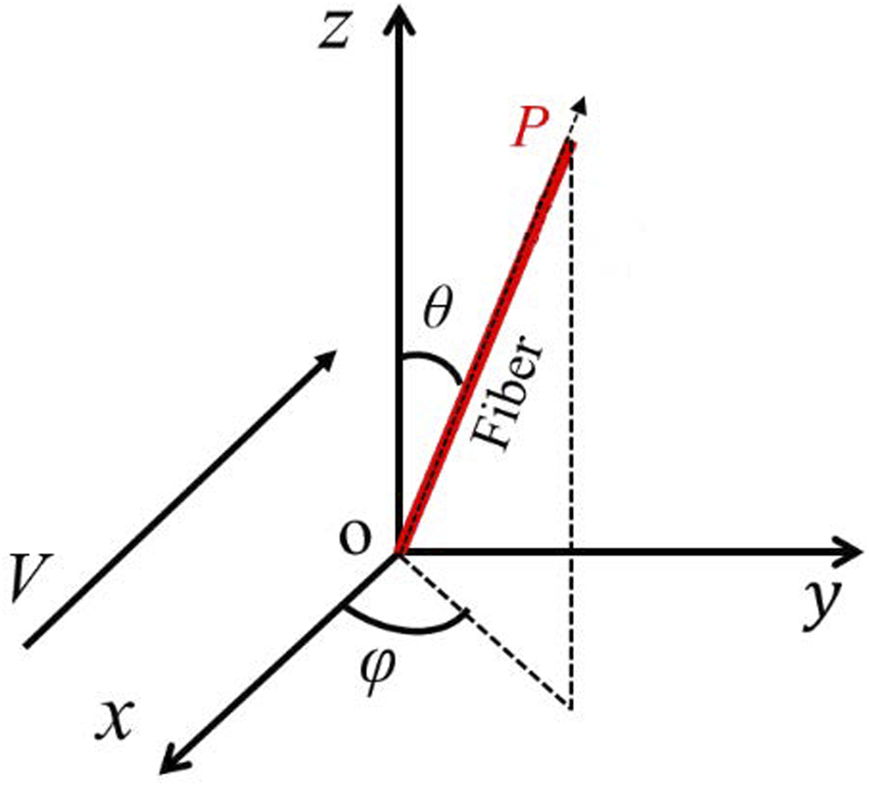

In order to use formula (8) to calculate the force exerted on the fiber in the three-dimensional space, the speed u needs to be decomposed into the component u_s parallel to the fiber axis and the component u_r perpendicular to the fiber axis.

\begin{array}{l} u_{s} = \dot{γ} ξ \sin^{2} θ \sin φ \cos φ \\ u_{r} = \dot{γ} ξ \sin θ \sin φ \sqrt{1 - \sin^{2} θ \cos^{2} φ} \end{array}}

(11)

Substitution of the u_r into formula (8), the force of the flow field on the fiber in the absence of melt slip on the fiber surface can be obtained. Nevertheless, during the actual melt injection process, the fiber-melt contact surface may slip. As a consequence, it is necessary to introduce the slip coefficient μ to meet the condition that the synthesis speed on the fiber surface is equal to zero. From this, the actual value of g(ξ) is

g (ξ) = \frac{- 8 π η \dot{γ} a \sin θ \sin φ \sqrt{1 - \sin^{2} θ \cos^{2} φ} (1 - μ)}{2 \ln (2 β) + 1}

(12)

Consequently, the force perpendicular to the axis exerted on the fiber by the flow field can be written as:

F = \frac{16 π η \dot{γ} a^{2} \sin θ \sin φ \sqrt{1 - \sin^{2} θ \cos^{2} φ} (1 - μ)}{2 \ln (2 β) + 1}

(13)

In order to determine whether the fiber is broken, the constrained fiber is treated as a cantilever beam, and the bending damage of fiber is transformed into a bending problem of the cantilever beam. When force F acts evenly on the fiber axis, the maximum tensile stress of the fiber is

σ_{\max} = \frac{M_{\max}}{W}

(14)

where M_max is the maximum bending moment and W is the bending section coefficient. They are calculated by formula (15) and (16), respectively

M_{\max} = \frac{1}{2} F L

(15)

W = \frac{I_{z}}{b} = \frac{π b^{3}}{4}

(16)

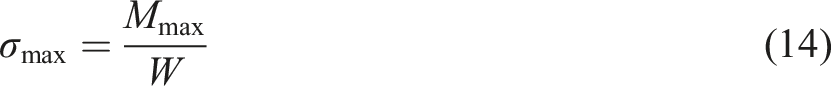
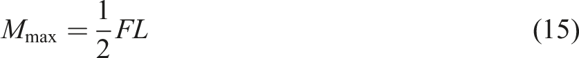
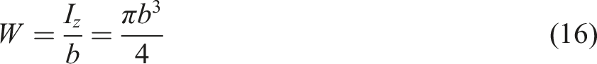
I_z is the moment of inertia of the section. Therefore, the value of maximum tensile stress is

σ_{\max} = \frac{64 \dot{γ} η β^{3} \sin θ \sin φ \sqrt{1 - \sin^{2} θ \cos^{2} φ} (1 - μ)}{2 \ln (2 β) + 1}

(17)

From the above result, it can be seen that the tensile stress applied to the fibers in the flow field is positively correlated with the melt viscosity and shear rate.

The critical length of fiber breakage

It can be seen from formula (17) that the maximum tensile stress σ_max exerted by the flow field on the fiber increases with the increase of its length. When σ_max exceeds the tensile strength σ_c of the fiber, the fiber breaks. Here, the critical length L_c of fiber breakage is defined as the maximum residual length, when the fiber is no longer broken under a certain orientation and shear stress. At this point, σ_max is equal to σ_c, and then there is the following equation (5)

σ_{c} = \frac{64 \dot{γ} η {β_{c}}^{3} \sin θ \sin φ \sqrt{1 - \sin^{2} θ \cos^{2} φ} (1 - μ)}{2 \ln (2 β_{c}) + 1}

(18)

where the critical aspect ratio β_c can be obtained by solving equation (18) using numerical methods. As a result, L_c of the fiber can be calculated by equation (19)

L_{c} = 2 β_{c} b

(19)

The above formula indicates that the critical length L_c is determined by the shear stress of the flow field acting on the fiber and its own orientation state. For a stable shear flow field, when θ = 90° and φ = 90°, the tensile stress suffered by the fiber reaches its maximum value. In this case, the calculated L_c is also the limit length that the fiber can be broken in the flow field and only when the fiber the length of the fiber is greater than this limit value. Consequently, L_c is also the standard for measuring whether the fiber is broken in its current orientation state.

Computational analysis

To better understand the effects of shear rate and fiber orientation on L_c, a calculation program for the above formula was developed via Python. The evolution of L_c was analyzed using long glass fiber 30% by weight and polypropylene (PP/30%LGF, Sabic 30YM240). Tensile strength σ_c and Radius b of this fiber are 3.5 × 10⁹ Pa and 10 μm, respectively. The viscosity of melt was calculated by the Cross-WLF, with the following formula

\begin{array}{l} η = \frac{η_{0}}{1 + {(\frac{η_{0} \dot{γ}}{τ^{*}})}^{1 - n}} \\ η_{0} = D_{1} \exp {- A_{1} (T - T^{*}) / [A_{2} + (T - T^{*})]} \end{array}}

(20)

where η is the viscosity, η₀ is the zero-shear viscosity,

\dot{γ}

is the shear rate, τ* is the critical shear stress, n is the power law exponent, T is the melt temperature, and T* is the glass transition temperature. D₁, A₁ and A₂ are constants related to the material. T*, n, τ*, D₁, A₁ and A₂ are 263.15 K, 0.2723, 73124, 7.91 × 10¹⁰, 23.528 and 51.6 K, respectively. Based on the experimental study of wall slip carried out by Zhuang et al.,³¹ the slip coefficient μ is taken as 0.329.

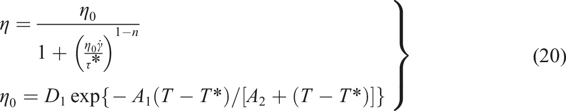
Figure 4 presents the evolution of L_c as the function of shear rate at different temperatures and orientation states. As is apparent from Figure 4, regardless of whether the melt temperature is 200 or 250°C, the critical length L_c gradually decreases with the shear rate and shear stress of the flow field. This indicates that increasing the shear rate causes the fiber to be more easily broken and the residual length shorter. It’s worth noting that, unlike the rapid decrease of L_c between $\dot{γ}$ = 1-400 s⁻¹, the reduction rate of L_c slows down rapidly after the shear rate reaches 401 s⁻¹, and eventually, its value remains relatively stable after $\dot{γ}$ = 800 s⁻¹. This suggests that the fiber is no longer susceptible to fracture following a certain reduction in length.

Figure 4.

The evolution of L_c as the function of shear rate at different temperatures and orientation states. (a) θ = 45° and φ = 45°, (b) θ = 90°, φ = 90°.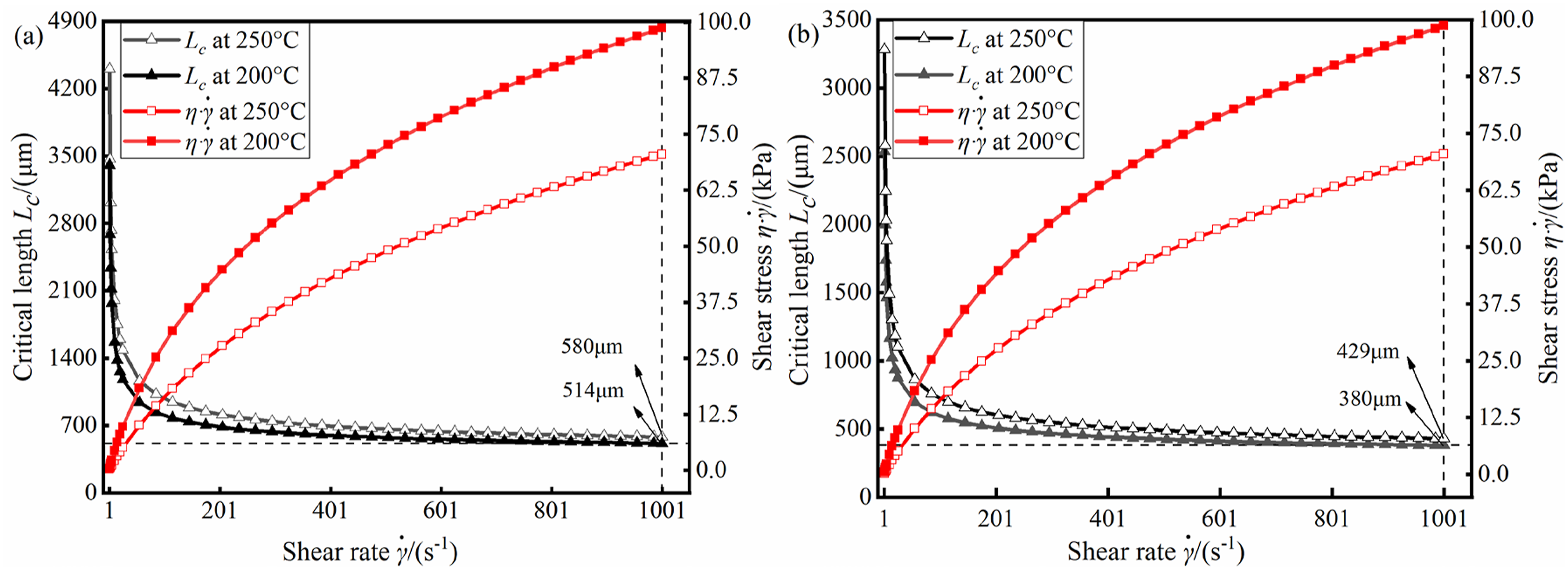

At the shear rate of 1000 s⁻¹, the fibers exhibited maximum tensile stresses at orientation angles θ and φ of either 45° or 90°. At this point, the L_c of the former drops to 580 μm and 514 μm at 200°C and 250°C, while the L_c of the latter drops to 429 μm and 380 μm. The actual shear rate of the mold cavity (exclusive of the pouring area) is typically less than 1000 s⁻¹, indicating that the above L_c is nearly the minimum fiber length that can be broken in the injection product. In early experimental studies, the range of minimum fiber residual length was reported to be approximately 0.2 to 0.6 mm. The findings of this paper provide a theoretical explanation for the varying calculations of the minimum fiber residual length in injection-molded products.^32–34

Apart from the shear rate, the L_c is also influenced by the orientation of the fibers. The results of the effect of fiber orientation on L_c at the melt temperature of 250°C and $\dot{γ}$ = 1000 s⁻¹ are given in Figure 5, where the values of θ and φ vary from 5° to 180°. In line with the findings presented in Figure 4(b), it is observed that the value of L_c is minimized when θ and φ are both at 90°. This indicates that fibers aligned along the y-axis bear the highest level of shear stress and are more susceptible to fracturing. Although the value of L_c is large when the fiber axis is near the x-z plane, the L_c of fiber is less than 1.4 mm for most orientation angles. The results demonstrate that existing analytical methods can be employed to quantitatively assess the range of fiber length distributions observed in injection-molded products, following the provision of the appropriate process parameters.

Figure 5.

The evolution of L_c as the function of fiber orientation at melt temperature of 250°C and 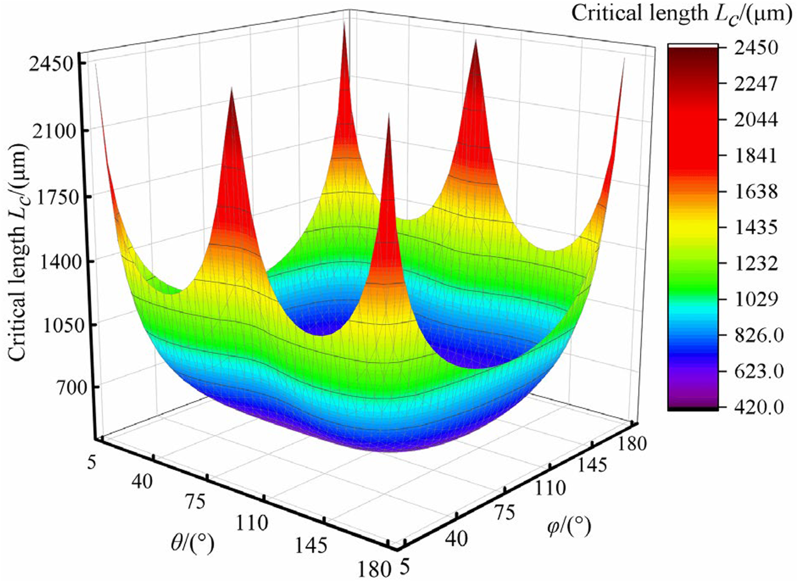$\dot{γ}$ = 1000s⁻¹.

Verification

Fiber length simulation

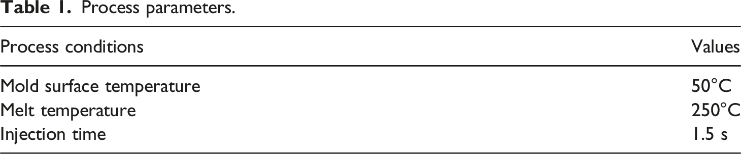
To obtain the fiber length distribution data of the whole product, the rectangular flat plate was divided into 115,559 tetrahedral grids, and 30 wt% long glass fiber reinforced polypropylene composite (LGF/PP, SABIC 30YM240) was used for injection filling simulation, with the gate in the middle of the long side, as shown in Figure 6. The injection filling process parameters are given in Table 1.

Figure 6.

Three-dimension mesh of thin-walled rectangular product (360 mm × 100 mm × 2.9 mm).

Table 1.

Process parameters.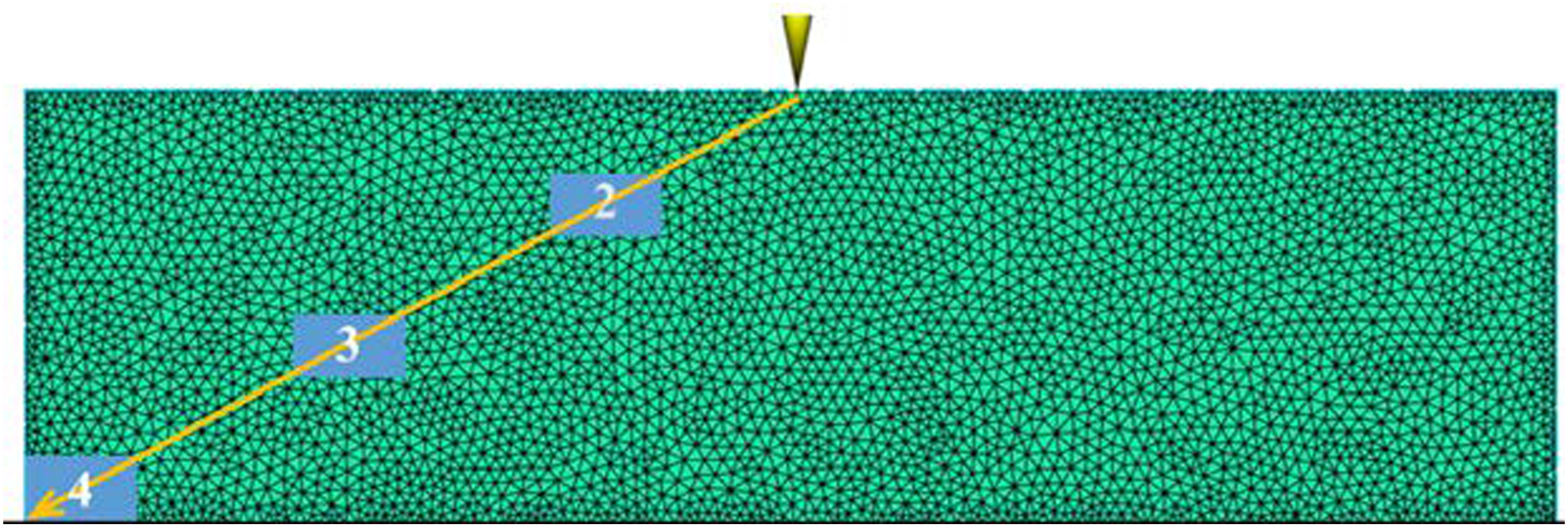

Process conditions	Values
Mold surface temperature	50°C
Melt temperature	250°C
Injection time	1.5 s

Based on the dynamic distribution results of melt temperature, shear rate and fiber orientation in the filling process obtained from the above flow analysis, the program developed by Python was used to calculate the fiber breakage critical length L_c of each grid element.

The fiber length at the gate obtained by the experimental method was denoted as [L_i]₀, representing the initial length distribution after the fiber entered the cavity. As the melt progressed through the cavity during the first filling time step, the initial length distribution [L_i]₀ flowed downstream with the molten material. At each downstream position, the flow field data was utilized to calculate the L_c. The comparison was made between the [L_i]₀ and L_c. If [L_i]₀ exceeded L_c, it means fiber breakage occurred. Consequently, a new fiber length distribution [L_i]₁ was established. In subsequent filling time steps, this process was repeated iteratively. After the ith filling time step, the previous length distribution [L_i]_i-1 continued to flow downstream with the melt. At the current position, fiber breakage was recalculated, leading to the formation of a new length distribution [L_i]_i. This iterative procedure was repeated until the entire cavity was filled, allowing the fiber length distribution data to be obtained throughout the product.

For the longest filling path shown in Figure 6, three positions were selected and numbered as samples 2, 3 and 4. Figure 7 depicts the predicted fiber lengths at the gate location and three sampling locations using the method described above. As shown in Figure 7, as the distance between the sampling point and the gate increases, the peak value of the fiber length gradually shifts to the left, and the fiber length at the peak value gradually decreases. This indicates that a greater distance from the gate results in a higher proportion of short fibers and a lower proportion of long fibers. There are two main reasons for this phenomenon. On the one hand, during the forward flow of melt, shear forces cause fibers to shorten. On the other hand, after the fibers break, one part continues to move forward with the melt, while another part is constrained by the frozen layer, resulting in a shorter length further away from the gate position.

Figure 7.

Quantity fraction distribution of fiber lengths for different samples: (a) Gate location, (b) Sample 2, (c) Sample 3, (d) Sample 4.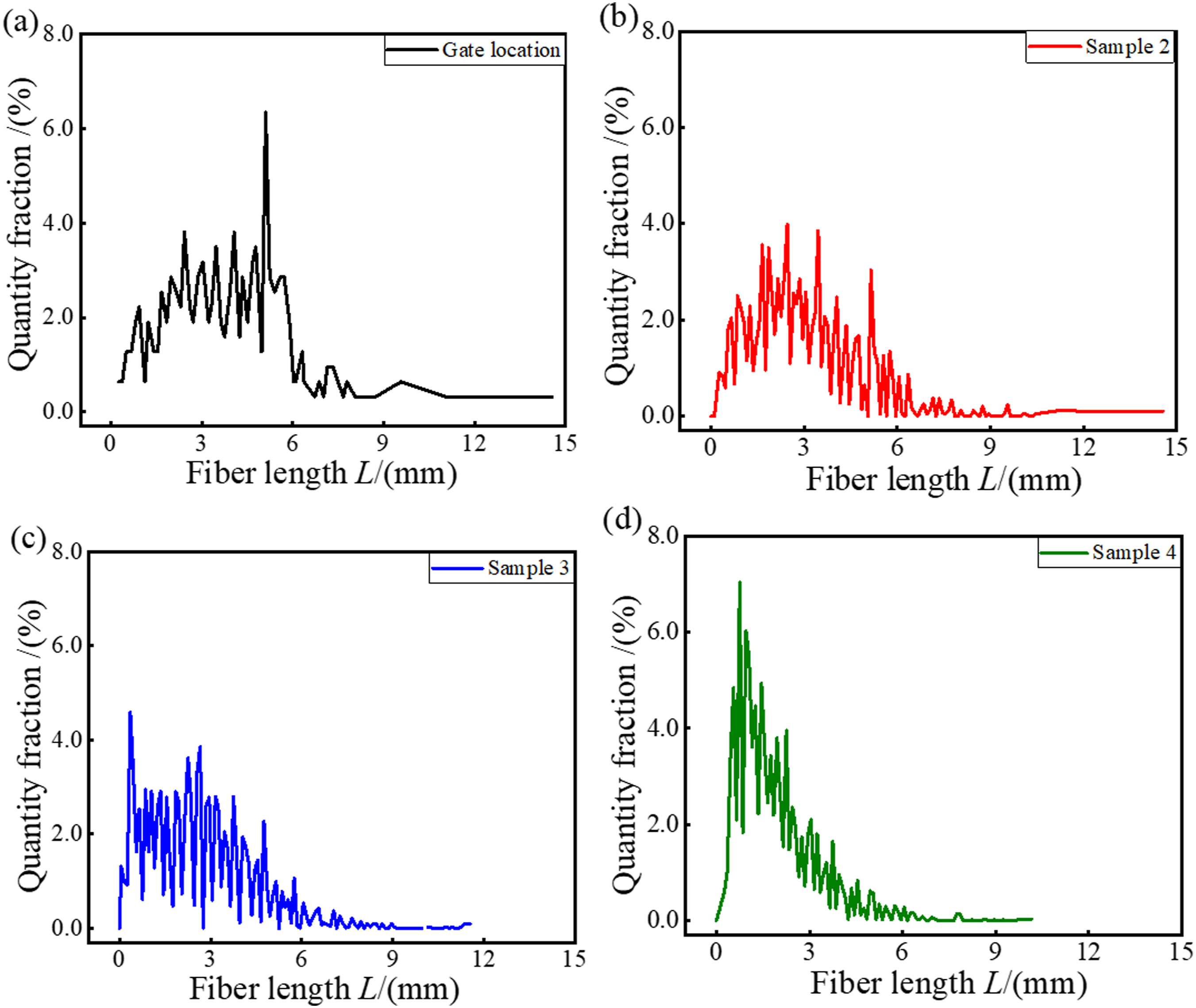

Experiment

To validate the method, a batch of rectangular thin-walled products was manufactured (as shown in Figure 8(a)). These rectangles were made from LFRT particles with an initial fiber length of 15 mm using the same parameters as the flow simulation.

Figure 8.

(a) Long fiber reinforced thin-walled product and (b) samples before calcination and (c) samples after calcination.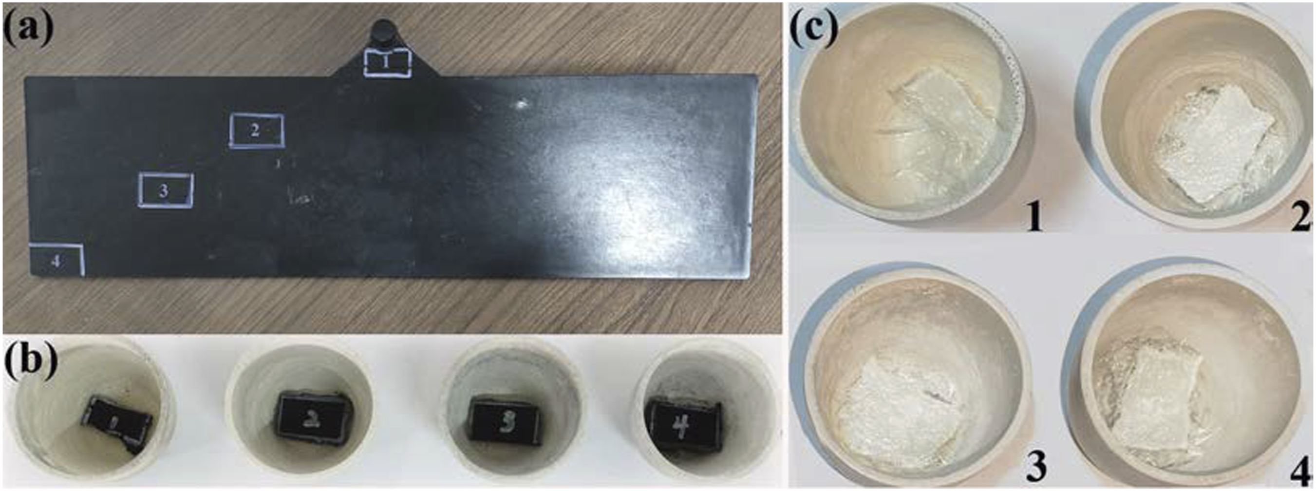

Based on the positions depicted in Figure 8(a), four samples with a length of 25 mm and a width of 15 mm were prepared from one product by using a wire saw (as shown in Figure 8(b)). Subsequently, they were calcined in a Muffle furnace at 400°C for 6 h and at 600°C for 1 h to achieve the separation of the fibers and the matrix. The appearance of the calcined sample is illustrated in Figure 8(c).

Fibers separated from the matrix were dispersed in deionized water, and their length and corresponding quantity were measured and counted using a high-precision fiber length analyzer (FASEP 3E-ECO, Germany). Micrographs for measuring and counting fiber length are shown in Figure 9. Figure 10(a) illustrates the quantity fraction of fibers at different lengths. The majority of fiber length in samples 1, 2, 3 and 4 are 5103, 2242, 750 and 713 μm, respectively. In general, as the distance between the sampling location and the injection port increases, there is a gradual decrease in the fiber length at the peak of the number fraction. In other words, the sample that is further from the gate has a higher proportion of shorter fiber. The primary reason for this is that the longer the distance from the gate, the greater the flow path of the fiber within the mold cavity. Consequently, an increased exposure to shear forces results in a higher probability of fiber breakage and a more concentrated distribution of short fibers.

Figure 9.

Micrographs for measuring and counting fiber length. (a) Sample 1, (b) Sample 2, (c) Sample 3 and (d) Sample 4.

Figure 10.

Fiber length distribution at various positions: (a) Quantity fraction, (b) Volume fraction.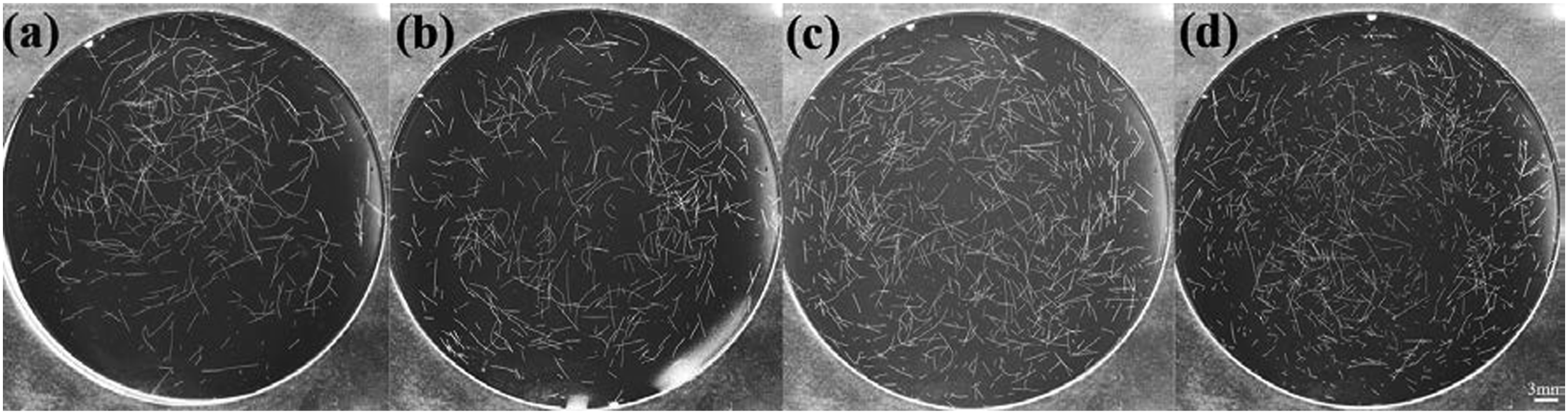

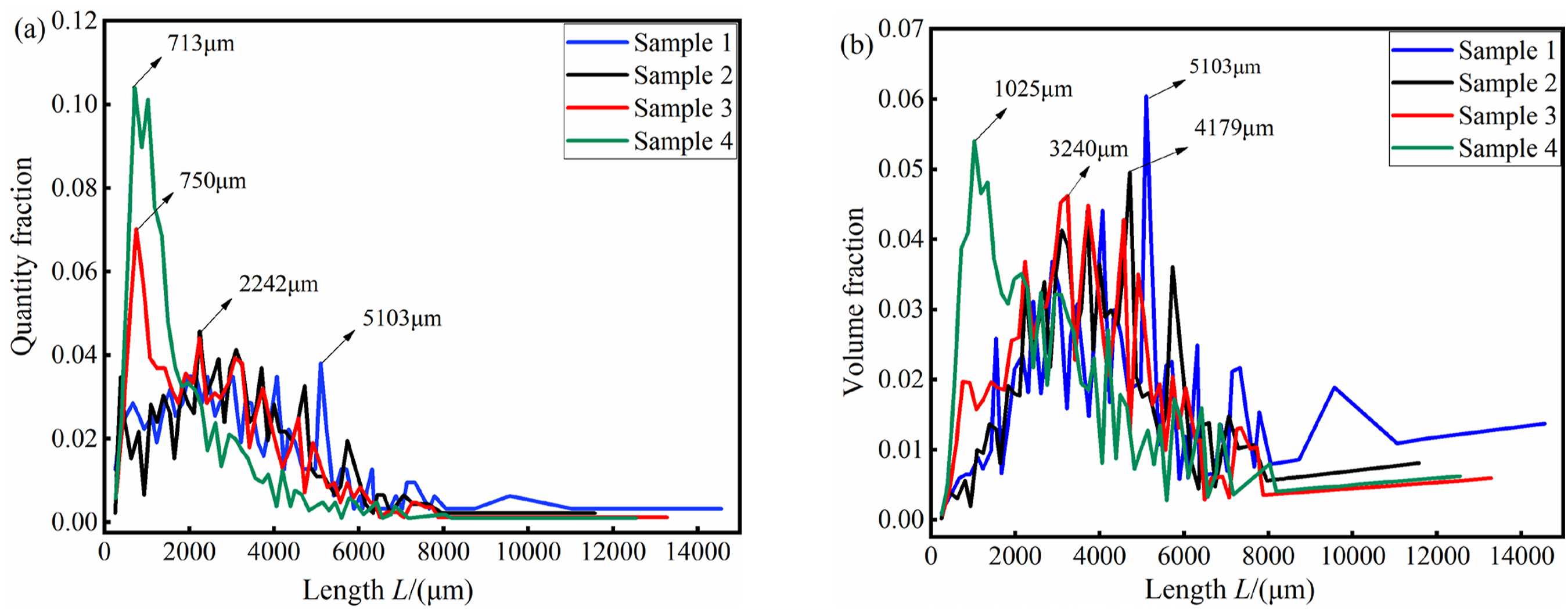
For the four samples, the maximum fiber lengths are 14.6, 11.6, 13.3 and 12.5 mm, while the minimum are 246, 250, 276 and 254 μm, respectively. This further illustrates that fibers are no longer easy to break after their lengths are reduced to a certain extent.

Figure 10(b), it can be observed that the fiber length at the peak volume fraction of each sample is greate provides the volume fraction distribution of fibers at different lengths and the results also show that the volume fraction of shorter fibers increases with the distance from the gate. By comparing Figure 10(a) and (b), it can be observed that the fiber length at the peak volume fraction of each sample is greater than that at the peak quantity fraction.

Figure 11(a) and (b) are the quantity average length L_n and weight average length L_w of fibers for each sample, respectively. Consistent with the findings mentioned above, both L_n and L_w exhibit a decrease as the distance between the sampling location and the injection gate increases. Additionally, the average length of weight for each sample is greater than the average length of quantity.

Figure 11.

Quantity average length (a) and weight average length (b) of fibers.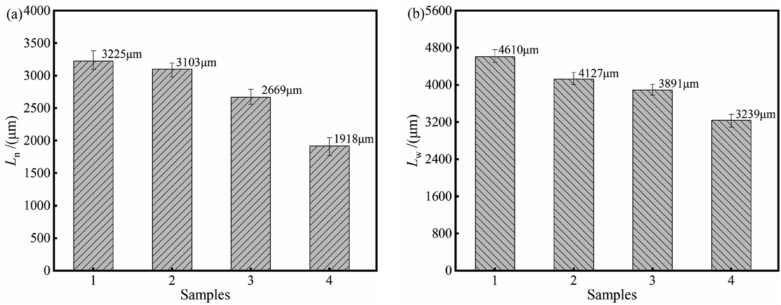

Comparison of results

Figure 12 shows the comparison of quantity fraction for each length interval between experimental and calculated data. The length distributions predicted for samples 2, 3 and 4 are in good agreement with the corresponding experimental results, as shown in Figure 12(a)–(c), respectively. The average prediction accuracy of samples 2, 3, 4 were 87.8%, 91.4% and 83.6%, respectively. Taking into account the impact of simulation errors in the temperature field, velocity field, and shear field on L_c calculation, these predictive results are considered to be optimal.

Figure 12.

Comparison of quantity fraction between experimental and calculated data: (a) Sample 2, (b) Sample 3, (c) Sample 4.

To further verify the reliability of the proposed method, Figure 13(a) and (b) show the comparisons of experimental and predicted data on number average length L_n and weight average length L_w, respectively. The relative errors of predicted L_n in samples 2, 3 and 4 are 3.2%, 2.5% and 1.0%, respectively, and that of predicted L_w are 1.5%, 2.4% and 10.5%. In general, this method can effectively predict the fiber length distribution of injection molded thin-walled products and provides important support for further accurate calculation of the mechanical properties of the products.

Figure 13.

Comparison of experimental and predicted data on number average length (a) and weight average length (b).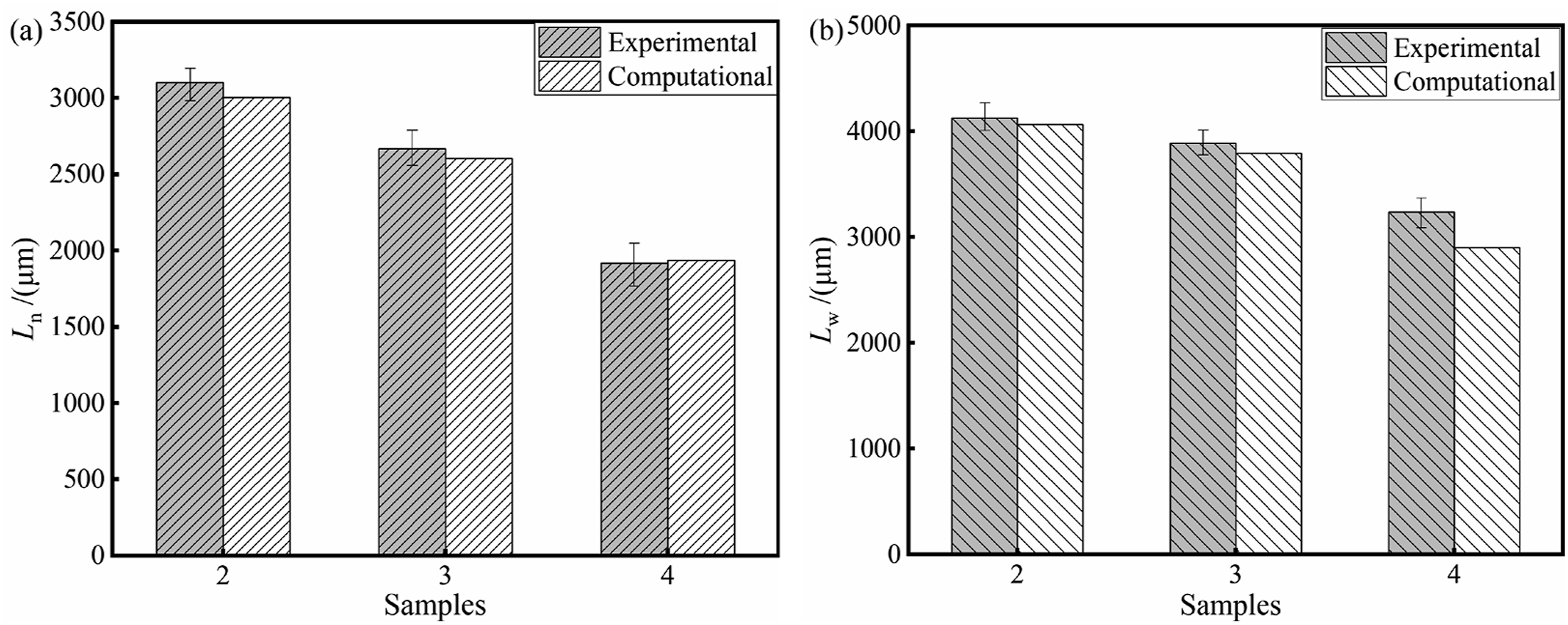

Conclusions

In this work, based on the OSEEN’s formula, a new model for calculating the critical length L_c is proposed to predict the fiber damage caused by the shear flow field in injection molding of thin-walled part.

The model was utilized to analyze the impact of shear rate and fiber orientation on L_c at various temperatures. It was found that the shear rate has a significant effect on L_c, with increasing shear rate, L_c decreases gradually, but the rate of decrease slows down over time, and the fiber is no longer easy to break after the fiber length is shortened to a certain degree. The analyses also suggest that the fibers orienting along the vertical shear direction are subjected to the greatest shear stress and are easiest to break. However, as the fiber orientation approaches closer to the shear direction, the force exerts on the fiber gradually diminishes.

A statistical experiment on the fiber length of typical long glass fiber-reinforced polypropylene thin-walled products was conducted. The average prediction accuracy of fiber length distribution at the three sampling locations was 87.8%, 91.4% and 83.6% respectively. The relative errors of number average leng L_n were 3.2%, 2.5% and 1.0%, while those of L_w were 1.5%, 2.4%, and 10.5% respectively. Apparently, the method proposed in this paper can effectively predict the fiber damage in injection molding thin-walled products, providing important support for further accurate calculation of the mechanical properties of products.

It is important to note that the model used in this study to predict fiber fracture is based on an idealized assumption, where defects are uniformly distributed along the fiber axis, and fractures are assumed to occur at the point of maximum flexural stress. However, in real-world applications, fiber defects tend to be non-uniformly distributed. The size and location of these defects have a significant impact on the failure behavior of fibers, often causing fractures at critical defect sites rather than at points of maximum bending stress. In future publications, our goal is to introduce a more advanced model that incorporates defects following a normal distribution along the fiber axis. This enhancement will allow for a more accurate prediction of fiber fracture behavior and the mechanical properties of composite materials under practical conditions, improving the applicability of the model to real-world scenarios.

Footnotes

Declaration of Conflicting Interests

The author(s) declared no potential conflicts of interest with respect to the research, authorship, and/or publication of this article.

Funding

The author(s) disclosed receipt of the following financial support for the research, authorship, and/or publication of this article: The authors gratefully acknowledge the financial support for this work by the National Key R&D Program of China (2019YFA0706802); Shenzhen Science and Technology Program (CJGJZD20210408092602006); the Open Fund of Yaoshan Laboratory; and the Major Research and Development Projects of Ningbo (2019B10117).

ORCID iD

Ming Huang

References

Zhiguo

Xianzhang

Yulong

, et al. Co-simulation technology of mold flow and structure for injection molding reinforced thermoplastic composite (FRT) parts. Adv Compos Hybrid Mater 2022; 5(2): 960–972.

Lin

Bao

. Combination and development of carbon filament tows: application of coextrusion with long fiber-reinforced thermoplastics. Polym Compos 2021; 42(9): 4199–4206.

Bechara

Goris

Yanev

, et al. Novel modeling approach for fiber breakage during molding of long fiber-reinforced thermoplastics. Phys Fluids 2021; 33(7): 073318.

Lou

Yin

, et al. Mechanical properties and fracture mechanism of a glass fiber reinforced polypropylene composites. J Wuhan Univ Technol -Mat Sci Edit 2020; 35(3): 629–634.

Wang

Chen

Hwang

, et al. Influence of back pressure and geometry on microstructure of injection-molded long-glass-fiber-reinforced polypropylene ribbed plates. Polym Test 2022; 116: 107797.

Shan

, et al. Analysis on effect of injection residual stress on impact resistance of composite wheel made of long glass fiber reinforced thermoplastic. Int J Crashworthiness 2021; 26(5): 515–525.

Wazeer

Das

Abeykoon

, et al. Composites for electric vehicles and automotive sector: a review. Green Energy Intell Transp 2023; 2(1): 100043.

Yao

, et al. Effect fiber length on mechanical and thermal properties of glass fiber reinforced polyphenylene sulfide composite. J Reinforc Plast Compos 2024: 07316844241232960.

Zhang

, et al. Effect of fiber content and fiber length on the dynamic compressive properties of strain-hardening ultra-high performance concrete. Construct Build Mater 2022; 328: 127024.

10.

Mei

Niu

, et al. Mechanical properties of cement matrix composites reinforced with polyoxymethylene fibers of different lengths. J Mater Civ Eng 2024; 36(3): 04023636.

11.

Wang

, et al. Preparation and properties of hybrid specific length carbon fiber thermoplastic composites by suspension method. Polym Compos 2024: 28318.

12.

Gao

Xiao

. Effect of glass fibers length on the properties of polytetrafluoroethylene composites reinforced by glass fibers and graphite: experimental and simulation study. High Perform Polym 2022; 34(3): 363–373.

13.

Huang

Peng

Hwang

, et al. The low breaking fiber mechanism and its effect on the behavior of the melt flow of injection molded ultra-long glass fiber reinforced polypropylene composites. Polymers 2021; 13(15): 2492.

14.

Hou

Chen

Liu

, et al. Fracture and orientation of long - glass - fiber - reinforced polypropylene during injection molding. Polym Eng Sci 2020; 60(1): 13–21.

15.

Huang

Peng

Hwang

, et al. Influence of low-fracture-fiber mechanism on fiber/melt-flow behavior and tensile properties of ultra-long-glass-fiber-reinforced polypropylene composites injection molding. J Polym Eng 2021; 41(2): 155–163.

16.

Zhang

Zheng

, et al. Effect of process parameters on the mechanical properties of fiber-reinforced thermoplastics fabricated by direct fiber feeding injection molding. Polym Eng Sci 2023; 63(8): 2457–2467.

17.

Yang

Zhang

, et al. Effect of screw configuration and screw speed on mechanical and rheological properties of glass fiber reinforced polyamide 66. Polym Mater Sci Eng 2010; 26(10): 118–121.

18.

. Study on injection molding of long glass fiber reinforced polypropylene[D]. Beijing: Beijing University of Chemical Technology, 2018.

19.

Zhou

, et al. Research on the effect of injection molding process on the properties and appearance of long glass fiber reinforced polypropylene. China Plast Ind 2018; 46(5): 85–88.

20.

Béreaux

Charmeau

Moguedet

. Modelling of fibre damage in single screw processing. Int J Mater Form 2008; 1(S1): 827–830.

21.

Durin

De Micheli

Ville

, et al. A matricial approach of fibre breakage in twin-screw extrusion of glass fibres reinforced thermoplastics. Compos Appl Sci Manuf 2013; 48: 47–56.

22.

Berzin

Beaugrand

Dobosz

, et al. Lignocellulosic fiber breakage in a molten polymer. Part 3. Modeling of the dimensional change of the fibers during compounding by twin screw extrusion. Compos Appl Sci Manuf 2017; 101: 422–431.

23.

Masubuchi

Terada

Yamanaka

, et al. Distribution function of fiber length in thermoplastic composites. Compos Sci Technol 2016; 134: 43–48.

24.

Huang

Zhao

. Novel modified distribution functions of fiber length in fiber reinforced thermoplastics. Compos Sci Technol 2019; 182: 107749.

25.

Ganesh

Obaid

Gillespie

. Experimental determination of bimodal strength distribution of S-glass fibers. Composites Part B-Engineering 2023; 254: 110559.

26.

Sasayama

Inagaki

Sato

. Direct simulation of glass fiber breakage in simple shear flow considering fiber-fiber interaction. Compos Appl Sci Manuf 2019; 124: 105514.

27.

Kang

Huang

Zhang

, et al. An effective model for fiber breakage prediction of injection-molded long fiber reinforced thermoplastics. J Reinforc Plast Compos 2020; 39(11–12): 473–484.

28.

Simacek

Advani

Gillespie

. Modeling short fiber deformation in dilute suspension: fiber deposition process. Compos Sci Technol 2022; 218: 109149.

29.

Ganesh

Abu Obaid

Gillespie

. Novel continuous fiber bending experiment to determine size- and spatial-distribution of surface defects in glass fibers. Compos Sci Technol 2023; 241: 110146.

30.

Burgers

Steketee

. On the motion of small particles of elongated form. Suspended in a viscous liquid[M]//Nieuwstadt F T M. In: Selected papers of J. M. Burgers. Dordrecht: Springer Netherlands, 1995, pp. 209–280.

31.

Zhuang

Wang

. Study on the effects of wall slip on melt filling flow in micro injection molding. China Mech Eng 2007; 18(16): 1995–1999.

32.

Zarges

Sälzer

Heim

. Correlation of fiber orientation and fiber-matrix-interaction of injection-molded polypropylene cellulose fiber composites. Compos Appl Sci Manuf 2020; 139: 106112.

33.

Stanford

Lovell

Thongpin

, et al. Experimental studies on the interfacial shear-transfer mechanism in discontinuous glass-fibre composites. Compos Sci Technol 2000; 60(3): 361–365.

34.

O’Regan

Akay

. The distribution of fibre lengths in injection moulded polyamide composite components. J Mater Process Technol 1996; 56(1–4): 282–291.

Critical length prediction for fiber breaking in injection molded of long-fiber reinforced thin-walled products

Abstract

Keywords

Introduction

Calculation model of fiber breakage

Disturbance of fibers to the flowing melt

Force exerted on the fiber in injection molding

The critical length of fiber breakage

Computational analysis

Verification

Fiber length simulation

Experiment

Comparison of results

Conclusions

Footnotes

Declaration of Conflicting Interests

Funding

ORCID iD

References