Sage Journals: Discover world-class research

Abstract

A new algorithm to generate Representative Volume Elements (RVEs) of random fiber distributions is presented in this study. The Random Sequence Expansion (RSE)_stirring algorithm generates the initial fiber random distribution. Subsequently, by stirring the generated fibers and highlighting the influence of fiber short-range spacing interactions, the method facilitates the capture of the real fiber distribution. To verify the soundness of the proposed algorithm, the RVE model, generated by the RSE_stirring algorithm, was analyzed using four statistical functions. The model was then statistically compared with the experimentally obtained real fiber distributions in a Completely Spatial Random (CSR) pattern. In this study, the equivalent modulus of the composite was also predicted using RVE and compared with the results predicted by other algorithms. The experimental and the predicted results showed a strong similarity.

Keywords

Fiber-reinforced composites representative volume elements random distribution finite element analysis elastic modulus prediction

Introduction

Carbon fiber-reinforced composites (CFRP) are becoming increasingly prevalent in the aerospace field because of their excellent properties such as lightweight, high strength, and impact resistance. CFRP consists of carbon fibers, which reinforce the mechanical properties of the composite, and a matrix polymer that binds the fibers together to protect them against the external environment.¹ Although the experimentally-derived composites are more accurate and reliable mechanically, such experiments often require huge financial and material inputs. With the development of computers and finite element technology, the fine-scale mechanical analysis of composites has gradually become a research hotspot. Further, analytical calculations or numerical simulations have been shown to be meaningful alternatives to experimental methods.²

The mesoscale mechanical analysis of fiber-reinforced composites is usually performed using their Representative Volume Element (RVE). Originally, Sun et al.³ conducted finite element analysis based on the RVE model to obtain the equivalent modulus of the unidirectional fiber composite. One of the most important issues for investigation based on the RVE model is the spatial arrangement of the fiber bundles. Initially, for the sake of analytical simplicity, a periodic and ordered fiber arrangement at the microscopic scale was assumed by Aghdam et al.⁴, who analyzed the RVE model using hexagonal arrays. However, subsequently, Zhang et al.⁵ found that the rectangular and the hexagonal arrays were inconsistent in predicting the transverse and the shear modulus, and the periodic array model was less accurate compared with the random model. Trias et al.⁶ found that matrix cracking and damage were underestimated by models with periodic fiber distribution compared with random distribution models as the real distribution of fibers was also random and disordered. Further, Segurado et al.⁷ proposed another technique to randomly generate fibers, known as the Strauss “hard-core” algorithm, also known as the Random Sequential Adsorption (RSA) algorithm. It ensures equal probability of generating each coordinate point within a specified range, without overlapping fibers. The technique is limited by the fiber content, which reached only about 50%, while in reality, it often reaches 60% or higher. Therefore, additional studies are ongoing to improve the content of the randomly generated fiber structures to levels higher than 60%.

The three classic methods to generate RVE models for random fiber distributions are as follows:

1) Perturbation method. As defined by Wongsto et al.⁸ it is based on fiber generation in a hexagonal periodic array via random size perturbation displacement, which leads to RVE with high levels of randomly distributed fiber content. Subsequently, Balasubramani et al.⁹ used the perturbation method to evaluate the effect of RVE aspect ratio on the predicted elastic modulus.

2) Nearest Neighbor Algorithm (NNA). Vaughan et al.¹⁰ combined simulation and experimental statistics to build an RVE model with geometric characteristics similar to those of the experimental sample. Ge et al.¹¹ used the NNA algorithm to evaluate the effect of interface parameters on the predicted elastic modulus.

3) Random Sequence Expansion (RSE) algorithm. Lei et al.¹² generated a stochastic distribution model with a high fiber volume fraction by adjusting the inter-fiber distance parameter. Subsequently, Kim et al.¹³ predicted the mechanical properties of unidirectional composites using convolutional neural networks (CNN) for the RVE model generated by the RSE algorithm.

Thus, a suitable algorithm for generating the RVE model plays a crucial role in the subsequent study to predict the elastic modulus. New algorithms, such as Random Microstructure Generation (RMG) by Melro et al.,¹⁴ Hard-Core Optimization Algorithm (HCOA) by Liu et al.,¹⁵ and an adaptive RVE model based on molecular dynamics and evolutionary periodic boundary algorithms by Qu et al.¹⁶ However, all of these aforementioned algorithms were too complex and difficult to promote.

Therefore, several studies have subsequently optimized and improved the classical algorithm. Wang et al.¹⁷ improved the NNA by adding the statistical properties of the actual fibers using scanning electron microscopy. Subsequently, they introduced probability equations to resolve the low approximate fiber distribution generated by the original NNA; however, the new method still failed to resolve the operational complexity. Liu et al.¹⁸ proposed a new RSA algorithm based on Boolean operation to generate the RVE containing non-overlapping fibers. Even though this algorithm shortens the modeling time by avoiding repeated cycles of running calculations, the algorithm does not consider the statistical elements of the actual fiber distribution.

Consequently, the main objective of this study was to propose an improved RSE method, called RSE_stirring algorithm, to generate an RVE model with high content. This algorithm, not only generates RVE rapidly and efficiently, but also overcomes the problem of single-fiber “drift” and fiber clustering phenomenon generated by the original RSE method. Thus, the obtained RVE is consistent with the real-world scenario. Subsequently, the RVE generated by the RSE_stirring algorithm was used for statistical analysis and prediction of elastic constants of composites. It was also compared with other algorithms as well as experimental results, reflecting the power of this algorithm.

The RSE_stirring algorithm is currently used in classical, unidirectional, continuous fiber composites. However, it should not be restricted to a single type, such as the Tailorable Universal Feedstock for Forming (TuFF) material, where Yarlagadda et al.¹⁹ demonstrated the potential to achieve composites of recycled discontinuous fibers with properties comparable to those of continuous fibers. Heider et al.²⁰ quantified the microstructural characteristics of experimentally obtained discontinuous composites represented by Tuff via statistical formulation. In future studies, the RVE model generated by discontinuous fibers should also be considered using the RSE_stirring algorithm.

This study is further divided as follows: section 2 discussing the development of the algorithm; section 3 dealing with statistical analysis; section 4, the prediction of the elastic properties of the system; and section 5, which summarizes the obtained results and proposes future perspectives.

Development of algorithm

The initial version of the RSE algorithm represents a random distribution model that produces high content of fiber volume fractions by adjusting the inter-fiber distance. The main limitation of this algorithm is that it does not analyze the real-world effects of microscopic distribution and the tendency to produce fiber clusters and free fibers. In addition, Valentin²¹ found that the local fiber aggregation introduces additional stress gradients, which play an important role in failure.

Therefore, the proposed RSE_stirring algorithm based on the advantages of RMG and NNA methods incorporates targeted fiber stirring, mobilizes each fiber to move toward the nearest and second nearest neighboring fibers, highlights the influence of fiber short-range spacing interactions, improves the long-range spacing fiber clusters and fiber drift. It also retains the simplicity and rapid modeling of the RSE algorithm. The flowchart of the RSE_stirring algorithm is presented in Figure 1. The different layers of the RSE_stirring algorithm are indicated.

Figure 1.

Flowchart of the RSE_stirring algorithm.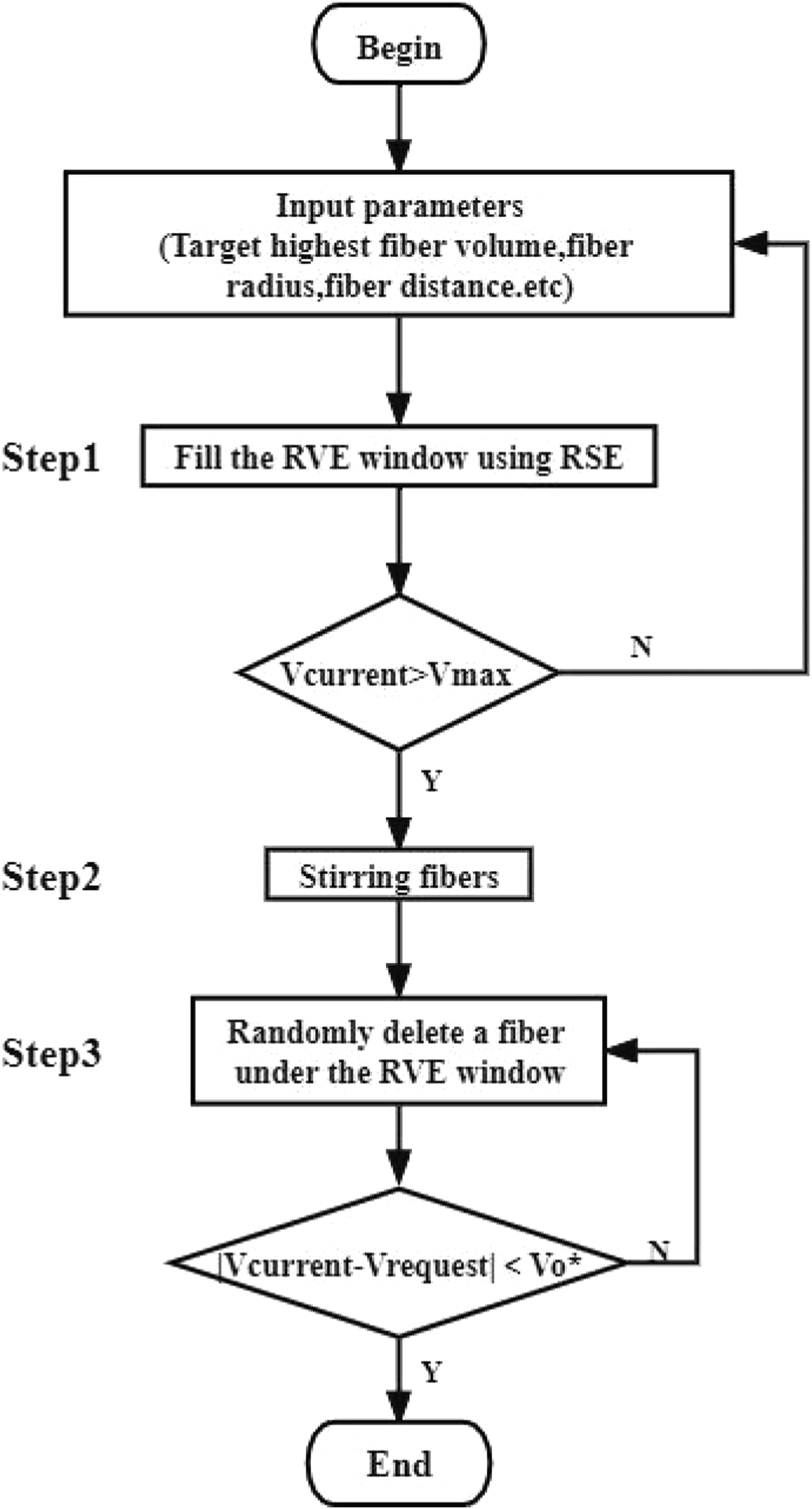

Step 1

RSE generates fibers

The following steps represent the procedure of the RSE algorithm. In addition, Figure 1 shows the outcome of these steps:

[1] Generate a random coordinate (x₁, y₁) within the RVE window (a*b) to serve as the first fiber;

[2] Search randomly around the first fiber and generate the location of the second fiber (x_2,y₂). It is obvious that:

x_{2} = x_{1} + (l_{1} + r_{1} + r_{2}) * c o s θ_{1}

(1)

y_{2} = y_{1} + (l_{1} + r_{1} + r_{2}) * s i n θ_{1}

(2)where r₁ and r₂ are the radii of the two fibers, respectively; l₁ is a random distance between

l_{\min}

and

l_{\max}

(representing the minimum and the maximum distances between two fibers), where

l_{\min}

is generally determined experimentally and

l_{\max}

determines the maximum possible fiber content of RVE. The relationship between all these variables is represented by:

{4 l}_{\min} + l_{\max} \approx (r_{1} + r_{2}) / 4

(3)

The direction of the second fiber ( $θ_{1}$ ) is randomly obtained in the range of [0, 2π] (refer to Figure 2(a) and (b));

[3] Repeat steps [2] to search and generate the position of the third fiber (x₃,y₃) (as shown in Figure 2(c)), and so on, where the other fibers are continuously generated until the maximum search time N_max (generally equal to 50) is reached. At this point, no new fibers can be generated around the first fiber (x₁,y₁). In order to maintain the geometric periodicity, if a fiber intersects the boundary, the interior where it is located is retained and the remaining portion is moved to the other side of the corresponding RVE window (as shown in Figure 2(d));

[4] Repeat steps [2] and [3] with the second fiber (x₂,y₂) that acts as the center. Then, the step [4] is repeated for each subsequent fiber until the complete RVE window is filled. During fiber generation, the fiber-to-fiber spacing must always remain greater or equal to the minimum spacing.

Figure 2.

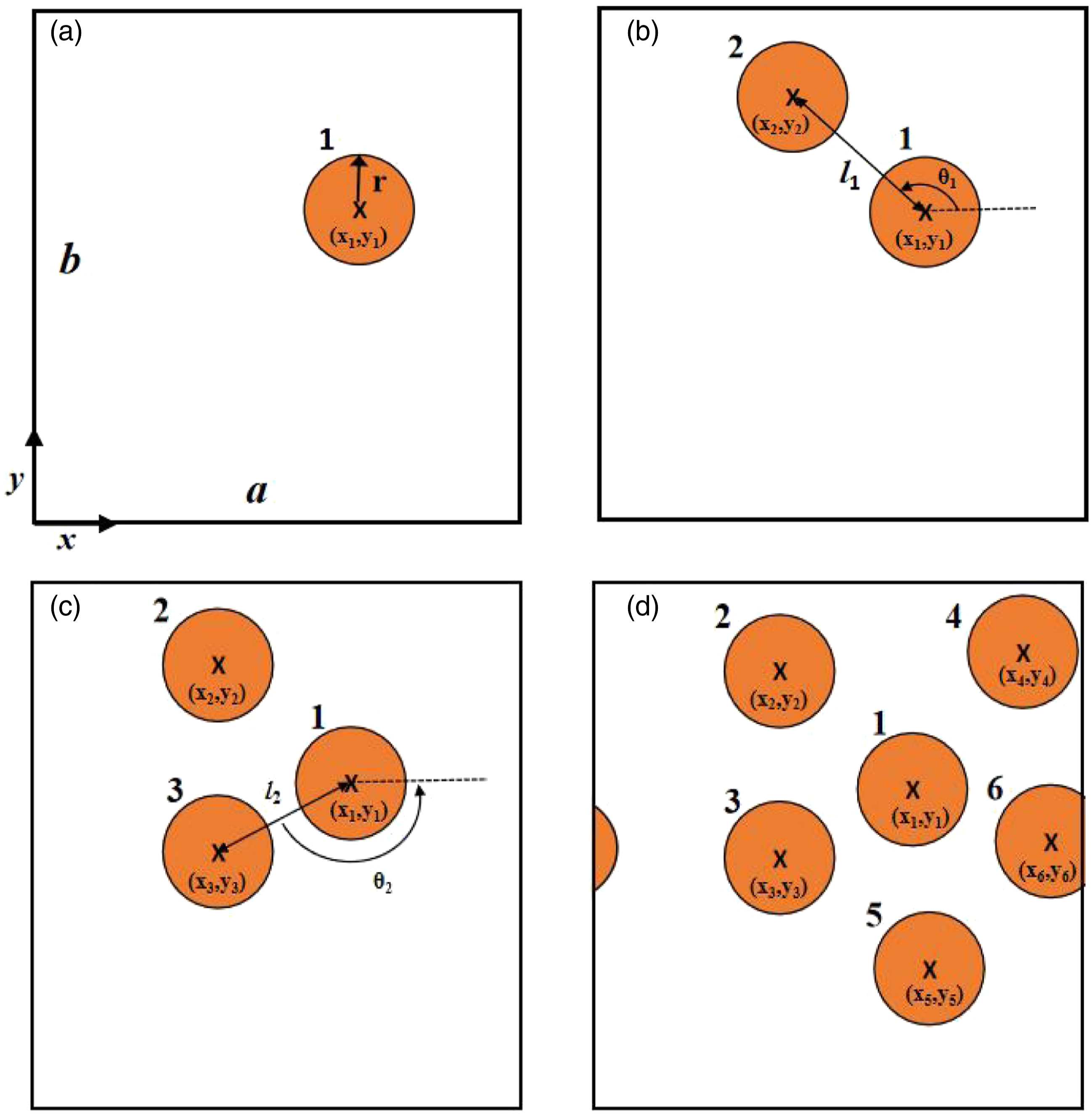
Random fiber generation using RSE method.

Step 2

Stirring fibers

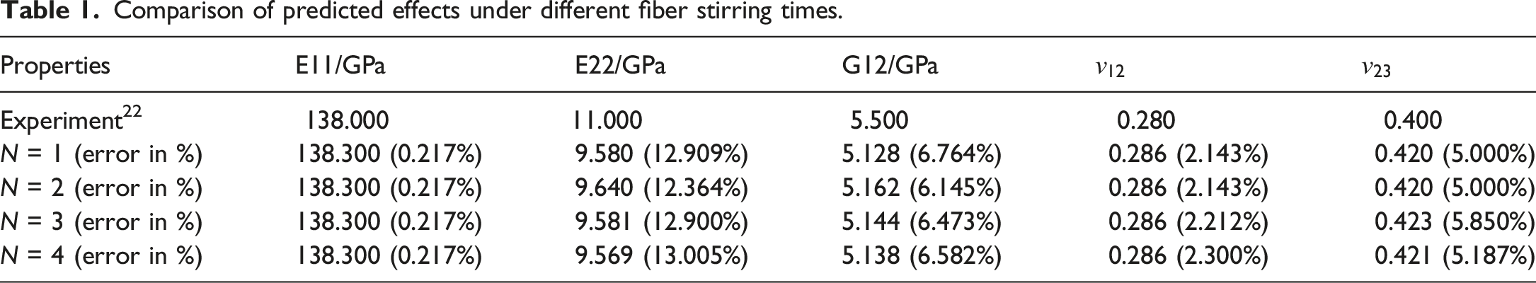
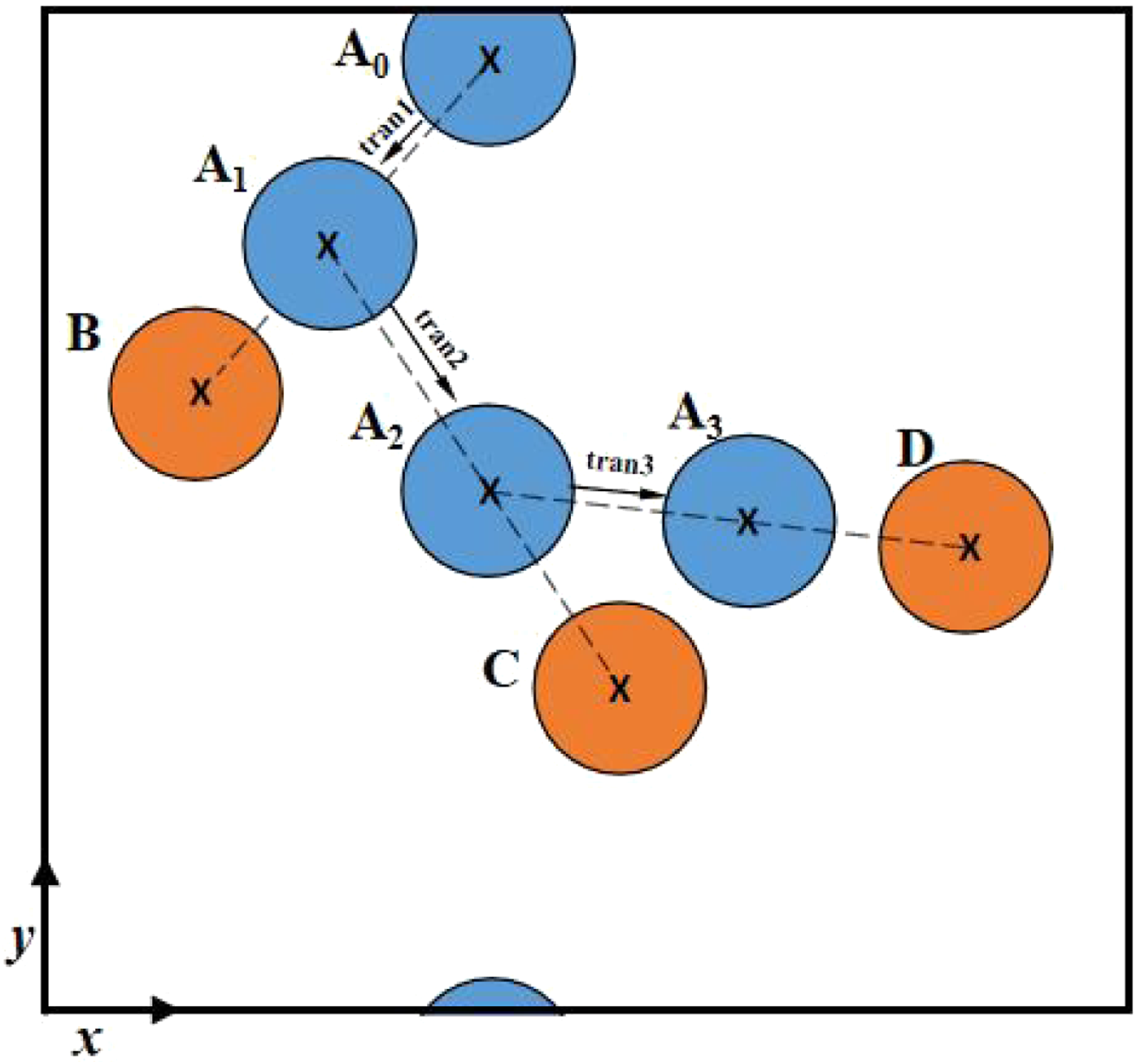
By adjusting the fiber spacing, the fiber stirring step can reduce the “fiber clustering” phenomenon. It can also increase the randomness of the long-range fiber distribution. The stirring process is presented in Figure 3.

[1] Stir the fibers generated in step 1-RSE generates fibers as shown in Figure 3. The window contains four fibers, A, B, C and D. During the fiber stirring, only a single fiber is moved, while the other fibers remain stable. Taking the first stirring of fiber A as an example, where fiber A₀ is the starting position of fiber A, A₀ is moved toward its nearest fiber (fiber B). The direction of movement is the direction vector of trans1 , and the moving distance length is a randomly generated value in the range of [0, $l_{A_{0} B} {- l}_{\min}$ ], which ensures the randomness of fiber distribution; thus, fiber A is moved to position A₁;

[2] During the second stirring of fiber A, the reference fiber in the first stirring (fiber B) is not considered. Thus, fiber A₁ seeks and moves towards its nearest fiber (fiber C). Similarly, the direction of movement is the direction vector of trans2; the moving distance is a randomly generated value in the range of [0, $l_{A_{1} C} {- l}_{\min}$ ]. Thus, fiber A is moved to the position A₂;

[3] Similarly, during the second stirring of fiber A, the reference fiber in the first stirring is not considered (fibers B and C). The fiber A₂ goes to the nearest fiber (fiber D) while passing through A₃. Theoretically, fiber A can continue to be stirred N-1 times (N being the number of valid RVE fibers, i.e., the number of fibers whose circle center coordinates within the RVE window), which leads to a significant increase in computing and modeling time. Considering that the degree of calculation is closely related to fibers stirring, we find the optimal number of stirring times from N = 1 to N = 4 to shorten the modeling time and improve the calculation efficiency. Discussing four different stirring times, we took five RVE models with fiber content of 60% for each type and obtained the mean and error of their predictions, respectively, and the results are shown in Table 1. The detailed procedure for predicting the modulus is referred to in Part IV of this paper - Prediction of elastic properties. From Table 1, it can be observed that The longitudinal modulus values and Poisson’s ratio values of the four fiber stirring times were almost indistinguishable, but the predicted values of transverse modulus and shear modulus were significantly better than the other three fiber stirring times in terms of error magnitudes. Therefore, the best prediction is observed for N = 2. Subsequent discussion in this study is based on the two stirring times.

[4] When the stirring of fiber A is completed, the next fiber enters the cycle. The stirring standard consists of determining each stirring to identify the nearest fiber. The above operation is repeated until all fibers in the RVE complete stirring. Note that fiber overlap cannot occur during the stirring process.

Table 1.

Comparison of predicted effects under different fiber stirring times.

Properties	E11/GPa	E22/GPa	G12/GPa	$ν_{12}$	$ν_{23}$
Experiment²²	138.000	11.000	5.500	0.280	0.400
N = 1 (error in %)	138.300 (0.217%)	9.580 (12.909%)	5.128 (6.764%)	0.286 (2.143%)	0.420 (5.000%)
N = 2 (error in %)	138.300 (0.217%)	9.640 (12.364%)	5.162 (6.145%)	0.286 (2.143%)	0.420 (5.000%)
N = 3 (error in %)	138.300 (0.217%)	9.581 (12.900%)	5.144 (6.473%)	0.286 (2.212%)	0.423 (5.850%)
N = 4 (error in %)	138.300 (0.217%)	9.569 (13.005%)	5.138 (6.582%)	0.286 (2.300%)	0.421 (5.187%)

The step 2 in this study is based on the algorithmic ideas of RMG¹⁴ and differs partially from the proposed RSE_stirring algorithm, which covers a larger range of targeted stirring. Thus, the movement of mobilized fibers toward the nearest and second nearest neighbor fibers is enhanced. The connection between internal and boundary fibers, which is also consistent with the actual fiber distribution.

Figure 3.

Stirring the fiber A.

Step 3

Random removal of fibers

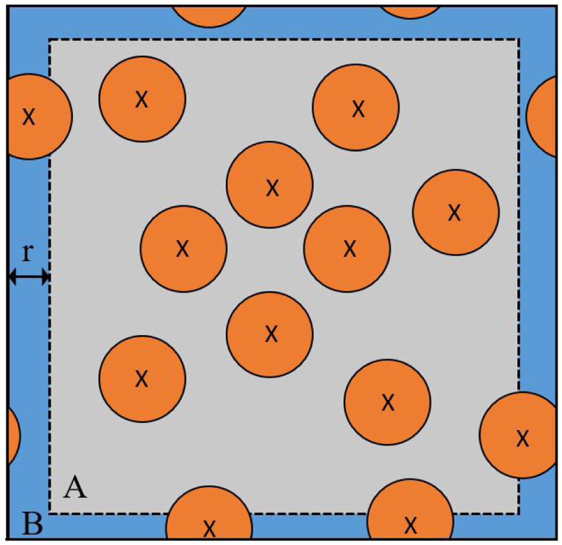
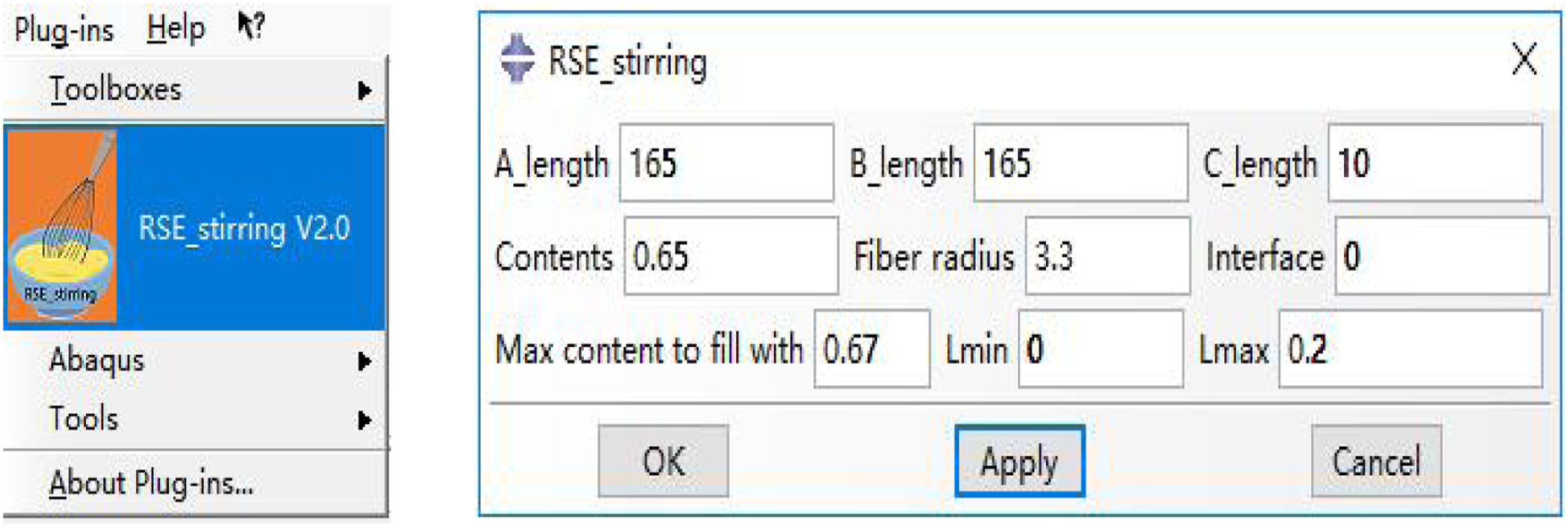
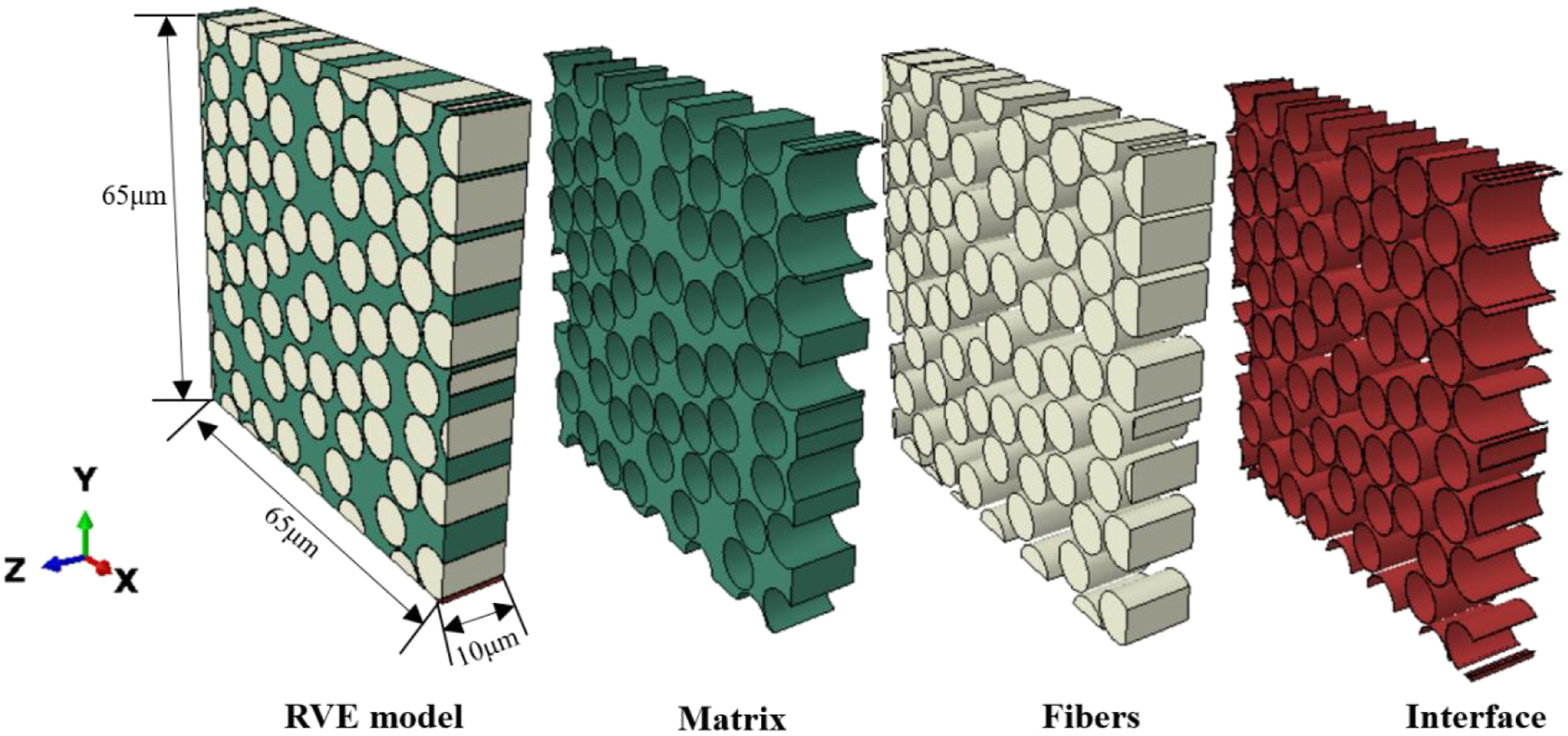
If the fiber content at this point is greater than expected, a number of fibers inside the RVE window will be removed randomly until the fiber content reaches the expected result. At this point, the RVE model is exported. Considering the periodic boundary conditions, the RVE window is divided into two regions A and B. Region A contains fibers that are completely distributed inside the RVE, whereas region B contains fibers on the RVE boundary, as shown in Figure 4. The letter r denotes the fiber radius. The steps for random fiber removal are described below:

[1] Count the number of valid fibers in regions A and B. As shown in Figure 4, the region A contains nine fibers and the region B consists of four fibers, yielding a total of 13 fibers (N = 13). Accordingly, the probability of obtaining any fiber in region A is 0.69, and the probability of finding it in region B is 0.31;

[2] Set a specific probability statistical function and output a random value among 0 (representing the occurrence of selected region A) or 1 (representing the occurrence of selected region B), according to the different probabilities of the two events. If zero is generated, one fiber in region A is randomly deleted. Conversely, when the value one is obtained, a single fiber in region B will be deleted;

[3] Determine if the current fiber content is at the expected content:

| V_{c u r r e n t} - V_{r e q u e s t} | < V_{0}

(4)

The first two steps are repeated until this condition is satisfied, and then the loop is ended to derive the RVE model.

The entire algorithm is written in Python code and displayed as a GUI plug-in for ABAQUS, as shown in Figure 5. The RSE_stirring algorithm is simple and user-friendly, both in terms of flow and GUI input parameters, and it allows the fibers to touch each other (when taking l_min = 0). As for the maximum volume fraction, it is approximately 68%. This plugin can also generate high-content RVE models with interfaces. Figure 6 represents a schematic of the RVE model with different constituent phase generated by the RSE_stirring algorithm for 61% fiber content.

During the preparation and production of carbon-fiber composites, a submicron-thick interphase between the fibers and the matrix is generated.23 The thickness of this interface specifically for CFRP materials was approximately 200 nm based on transmission electron microscopy (TEM) analysis,²⁴ resulting in a cylindrical shell. The interface properties strongly affect the mechanical properties of composites.²⁵ Composite failure analysis at the microscopic level is mainly reflected in matrix fracture and interface debonding. Therefore, the RSE_stirring algorithm was used to generate interfaces and for future studies involving the microscopic failure models of composites. Nevertheless, the interface has little influence on the prediction of elastic properties. Other algorithms²⁶ use the interface to predict the equivalent modulus. The results of prediction do not differ significantly from those not based on the interface. Therefore, the computational simplicity and subsequent models used to predict elasticity do not factor the interface.

The RVE model analyzed in this paper is the ideal model. In reality, it is impossible to avoid defects and voids generated by modern manufacturing techniques that aim to reduce production costs and time.²⁷ Zhang et al.²⁸ have used suitable statistical functions to analyze the voids in thermoplastic composites. While statistical void data are essential to capture the true behavior of the modeled material, it is also essential to model the shape voids used and determine the distribution format,²⁹ which requires further in-depth analysis.

Figure 4.

Dividing the RVE region into zones A and B.

Figure 5.

RSE_stirring main view.

Figure 6.

Representative Volume Element (RVE) model with different constituent phases.

Statistical characterization

In order to verify the statistical equivalence between the fiber distribution established by the RSE_stirring algorithm and the fiber distribution of the microscopic images of real composites,²² four statistical spatial descriptors³⁰ were used. This method analyses both the short- and the long-range interaction of fibers, including the nearest neighbor distances, the nearest neighbor orientation, Ripley’s K function, and the pair distribution function. To highlight the improvements in the existing method, the statistical properties of the proposed method and the original RSE were compared.

According to experimental observations,²² each fiber has a slightly different diameter. To simplify, the fibers in subsequent statistical data and the equivalent modulus calculation model were considered to have the same diameter and their average value was 6.6 μm. Further, Trias et al.³¹ showed that the larger the size of the RVE model, the more apparent the characterization. The width-to-diameter ratio of 50 is generally optimal and therefore, the RVE size used for the statistical analysis in this study was equivalent to 165 μm × 165 μm × 10 μm. The input variables were: r = 3.3 μm, the distance between two fibers ranged between 0 and 1.6 μm, and a total of 478 fibers were used. The four statistical properties were evaluated when considering a fiber content of 60.01% and the coordinate points of 20 sets of RVE models with similar content. Further, the Python language tool was used to determine the first two statistical properties; however, as the statistical properties three and four are based on their RVE periodic boundaries, the R language tool was used to the two statistical properties. In the following description, h denotes the distance between any two fibers and r denotes the fiber radius.

Nearest neighbor distance

The nearest neighbor distance is defined as the distance between the reference fiber and the nearest neighboring fiber, and its Probability Density Function (PDF)³⁰ reveals the interaction between the fibers, which is commonly used to characterize the arrangement of fibers. Whether the RSE stirring algorithm improves the cluster of long-range spacing fibers and fiber drift was further investigated. Figure 7(a) and (b) show the nearest neighbor and second nearest neighbor probability distribution functions, respectively. These functions are used to compare experimental results²² and the probability distribution of fiber distances between various simulation methods, including the original RSE and the RSE stirring algorithms.

Figure 7.

Comparison of PDF based on experimental characterization and results of simulation: (a) first nearest neighbor distribution and (b) second nearest neighbor distribution.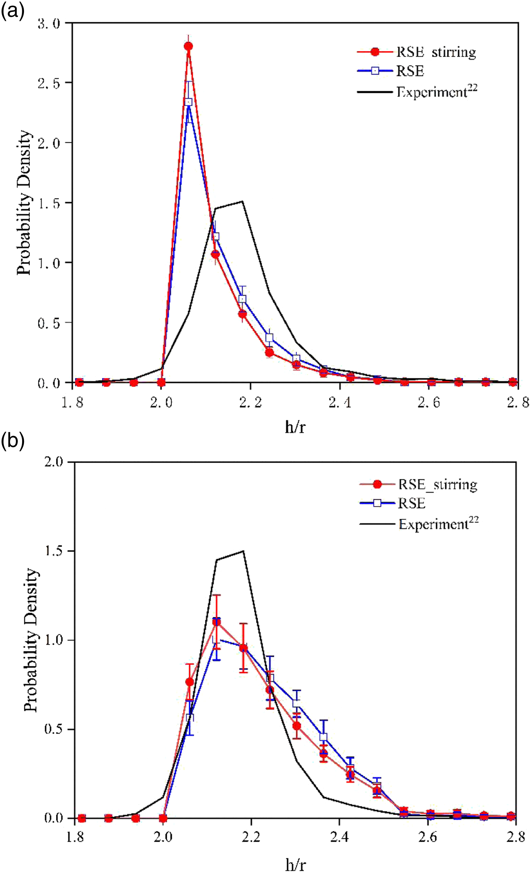

As shown in Figure 7, four conclusions can be drawn:

- 1) The experimental data differ from the data obtained from the two algorithms, mainly because the fiber distribution is generally not completely random in reality, and the nearest neighbor PDF does not follow the same form as the PDF of the Completely Space Random (CSR);

- 2) The abscissa is normalized as h/r, where r is the average fiber radius of 3.3 μm. Both RSE and RSE_stirring values of curves are zero when the h/r value varies between 0 and 2; while the experimental curve is not null. This indicates clearly the existence of experiments in which the distance h between two fibers is less than the sum of the two fibers’ radius, i.e., the phenomenon of fiber crossover occurs or the measured radius of both fibers is less than the average radius, neither of which occurs in the above two algorithms;

- 3) Concerning the nearest neighbor distribution (shown in Figure 7(a)), all three curves show peaks. The higher the peak, the more uniform the nearest neighbor distance between fibers. The highest observed peak of the RSE_stirring algorithm indicates clustering of the long-range spacing fibers and improved fiber drift;

- 4) Compared to the nearest neighbor distribution function, the peak of the curve of the next nearest neighbor distribution function is lower for both algorithms, and the general trend of the RSE_stirring curve fits the experimental curve more closely.

Nearest neighbor orientation

The nearest neighbor direction is the directional distribution of the undirected line connecting the center of the reference fiber and its nearest neighbor direction; it is generally described by the Cumulative Distribution Function (CDF).³⁰ The CSR is used to verify the randomness of its algorithm and has equal probability of occurring in the nearest neighbor direction at all angles, implying that the CDF is a diagonal line at 45°. Thus, Figure 8 shows that the curves carrying the RSE_stirring and the RSE algorithms are on almost the same straight line as the CSR curve for a complete round despite the slight vibration. Therefore, the randomness of the nearest neighbor fiber direction is still undamaged even with a high fiber content based on the RSE_stirring algorithm and additional stirring operation. This result further illustrated by the fiber distribution of the real experiment demonstrating an incompletely random phenomenon.

Figure 8.

Comparison between the nearest-neighbor direction cumulative distribution based on experimental characterization and simulation.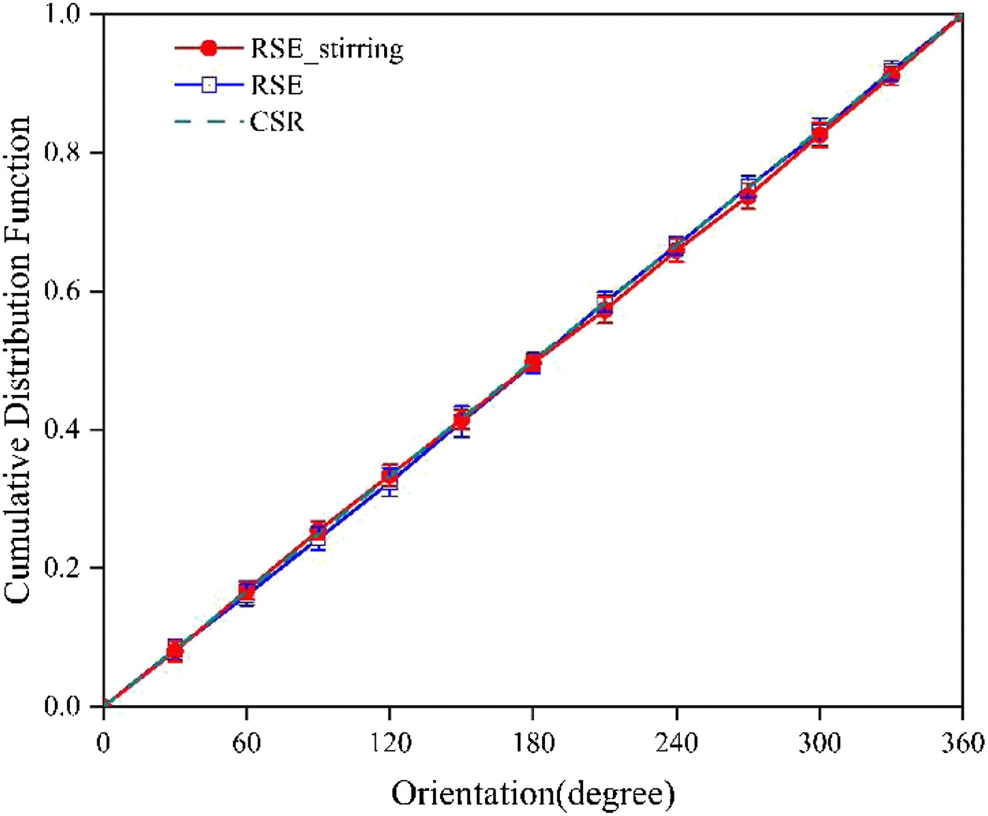

Ripley’s K function

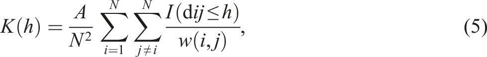
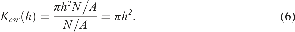
Ripley’s K function, also known as the second-order intensity function,³⁰ is one of the most informative descriptors of spatial patterns. It is defined as the ratio of the number of fibers within a radial distance h of any fiber to the number of fibers per unit area, and is expressed as follows³²

K (h) = \frac{A}{N^{2}} \sum_{i = 1}^{N} \sum_{j \neq i}^{N} \frac{I (d i j \leq h)}{w (i, j)},

(5)where A is the area of the RVE window and N is the total number of fibers in this window. I(

d_{i j} \leq h

) is the number of fibers within a given fiber radial distance, and w

(i, j)

represents the ratio of the circumference contained within the window to the entire circumference of the circle. For the CSR model, the equation (5) can be simplified as shown in equation (6)

K_{c s r} (h) = \frac{π h^{2} N / A}{N / A} = π h^{2} .

(6)

It is useful to analyze the fiber distribution by comparing the $K_{c s r} (h)$ curve using the CSR model with the $K (h)$ curves under other types. Based on statistical analysis,³⁰ if the $K (h)$ curve is higher than the $K_{c s r} (h)$ curve, fiber aggregation occurs, and vice versa, suggesting that this type of fiber distribution has a certain regularity. As shown in Figure 9(a), the $K (h)$ curves of the RVE fiber distribution were generated using the RSE_stirring, RSE and CSR models, as well as the experimentally obtained $K (h)$ curves. It is clear that all curves as a whole show a progressive increase with h/r.

Figure 9.

Comparison of K-functions for experimental characterization and simulation results: (a) 0 ≤ h/r ≤ 4; (b) 9 ≤ h/r ≤ 14; (c) 0 ≤ h/r ≤14.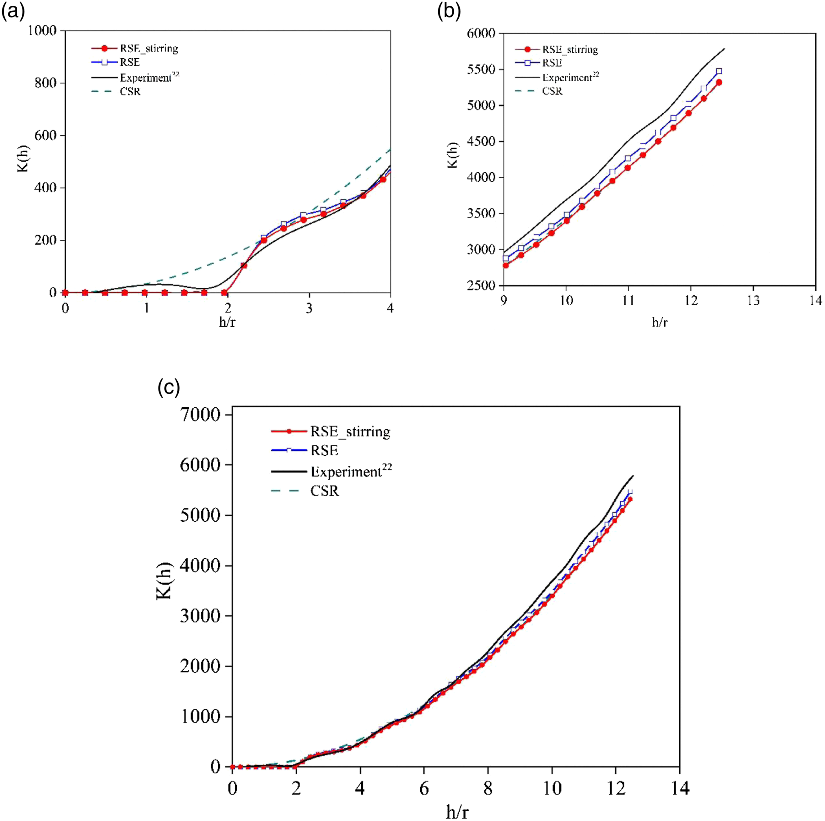

Figure 9(b) and (c) present the zoomed plots of Figure 9(a) when the h/r value varies between 9 and 14 and between 0 and 4, respectively. As shown in Figure 9(c), in the lower range (0 ≤ h/r ≤ 4), the three $K (h)$ curves are basically below the $K_{c s r} (h)$ curve, suggesting the absence of fiber aggregation. As shown in Figure 9(a) and (b), the two $K (h)$ curves representing the experimental and RSE algorithms, respectively, gradually lie above the $K_{c s r} (h)$ curve of the reference benchmark as the fiber distance increases, while the $K (h)$ curve representing the RSE_stirring is not generally higher than the $K_{c s r} (h)$ curve of the reference benchmark. As the fiber distance increases, the stirring step in the RSE_stirring algorithm significantly improves the fiber aggregation associated with the RSE algorithm, further illustrating the advantage of the RSE_stirring algorithm.

Pair distribution function

The pair distribution function, also known as the radial distribution function, is defined as the probability of finding an additional point in the annulus of the inner radius r and the outer radius r + dr. and is expressed as follows³²

g (h) = \frac{1}{2 π r} \frac{d K (h)}{d h}

(7)

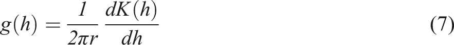
As shown in Figure 10, the value of the curve is almost zero at low distance range (0 < h/r < 2). The three curves fluctuate, and the amplitude of the oscillation gradually decreases. The simulated value at low distance range (2 < h < 3) differs between experimental results and the inputs of the two algorithms. In fact, the three curves gradually approach and converge to 1 as the distance h increases. As shown in Figure 10, the RSE_stirring algorithm does not destroy the randomness and that both algorithms fit the g(h) curves of the experimental values better over the long range of the fibers.

Figure 10.

Comparison of the radial distribution functions based on experimental characterization and simulation results.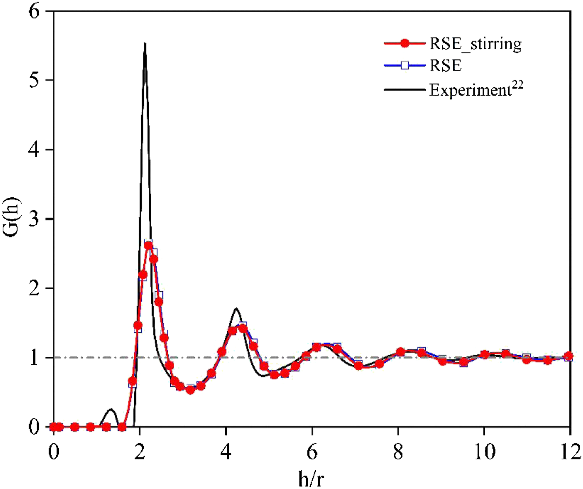

Prediction of elastic properties

The equivalent modulus of elasticity of the composite is the most intuitive parameter and the core metric determining the feasibility of the algorithm used to establish RVE. In this section, the effective elastic properties of the composites are predicted using the finite element method. The simulated results are then compared to the experimental results,²² the initial version of the RSE algorithm, the RSE_stirring algorithm, and the Modified NNA algorithm¹⁷ to verify the accuracy of the RSE_stirring algorithm.

Finite element model

In this article, we used the Python language tool to create a strongly optimized algorithm -- RSE_stirring plug-in, and build the RVE model in ABAQUS.³³

δ is defined as the length of the RVE model divided by the fiber radius.³¹ In this paper, the fiber radius is 3.3 μm. Therefore, the RVE size used for statistical analysis was 165 μm × 165 μm × 10 μm, i.e., δ = 50, with an average seed number of 1 μm, which resulted in a 3D model with about 160,000 elements carrying four elements based on the direction of thickness. Other algorithms²⁴ use a size of δ = 25, meaning that the RVE size is 82.5 μm *82.5 μm × 10 μm, and the same grid condition corresponds to a 3D model with about 40,000 elements. In order to determine the size with the best calculation time and the predictive effect among the two different sizes based on δ = 50 and δ = 25, five different RVE models with 60% fiber content for each size were used for prediction simulation in a comparative study. All runs were performed in a desktop computer with an i5-8500 3.0 GHz processor, 16 G RAM 512G SSD, and hyperthreading turned ON. The results are shown in Table 2. The difference in prediction based on the two sizes was basically small, suggesting that the size of δ = 25 also plays a role in the mechanical properties. Further, the calculation time of δ = 25 was 14.67 times shorter than that of δ = 50, so we used δ = 25 in the following prediction model based on size.

Table 2.

Comparison of simulation results for size ratio δ = 50 and δ = 25.

δ	E11/GPa (error in %)	E22/GPa (error in %)	G12/GPa (error in %)	$ν_{12}$ (error in %)	$ν_{23}$ (error in %)	Time(s)
50	137.700 (0.217%)	9.567 (13.030%)	5.131 (6.702%)	0.287 (2.357%)	0.425 (3.35%)	2715.8
25	138.300 (0.217%)	9.586 (12.851%)	5.247 (4.604%)	0.286 (2.143%)	0.421 (5.300%)	39,594.6

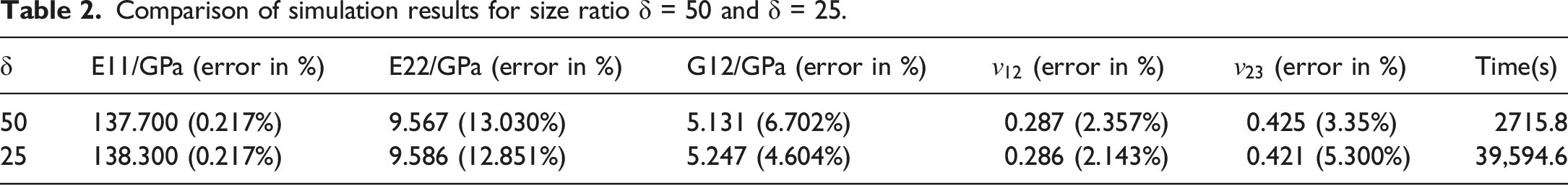
The RVE size of the model used for simulation in this section was 82.5 μm × 82.5 μm × 10 μm. The values of the input variables were defined. While r value was 3.3 μm, the distance between the two fibers ranged between 0.2 μm and 0.3 μm. A total of 120 fibers were used. The grid seed size was equal to the unit, and about 40,000 grid elements existed (C3D8R).

In order to ensure the alignment of the front and the back grid, the following steps were taken:

1. selection of the type of sweep mesh

2. moderately dense grid size to avoid concomitant increase in computational volume and meet the requirements of the periodic grid.

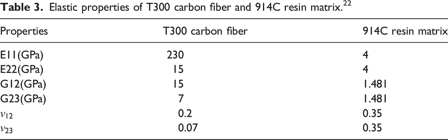
The fibers and the matrix were treated as transversely isotropic and anisotropic, respectively. The effect of the interface was neglected. The material properties were determined from the literature²² (Table 3). The outputs of the finite element model were compared with the experimental results²² of the carbon fiber-reinforced composite T300/914C with 60% fiber volume content.

Table 3.

Elastic properties of T300 carbon fiber and 914C resin matrix.²²

Properties	T300 carbon fiber	914C resin matrix
E11(GPa)	230	4
E22(GPa)	15	4
G12(GPa)	15	1.481
G23(GPa)	7	1.481
$ν_{12}$	0.2	0.35
$ν_{23}$	0.07	0.35

Periodic boundary condition

Setting periodic boundary conditions is crucial when predicting the elastic modulus.³⁴ Initially, Xia et al.³⁴ proposed a relatively well-developed periodic boundary condition to display the differences in displacement in a unified form for nonlinear analysis under arbitrary multi-axial loading. Omairey et al.³⁵ created a plug-in, called Easypbc, to integrate the surrounding conditions for predicting the elastic modulus. Easypbc can be currently applied only to the classical RVE model for unidirectional fibers and not to materials with a slightly more complex microstructure. Tian et al.³⁶ proposed a specific implementation of the algorithm to predict the elastic modulus for short fibers using the RVE model. Our study initially analyzed only fiber-reinforced composites. Additional studies may also incorporate complex RVE models for further analysis.

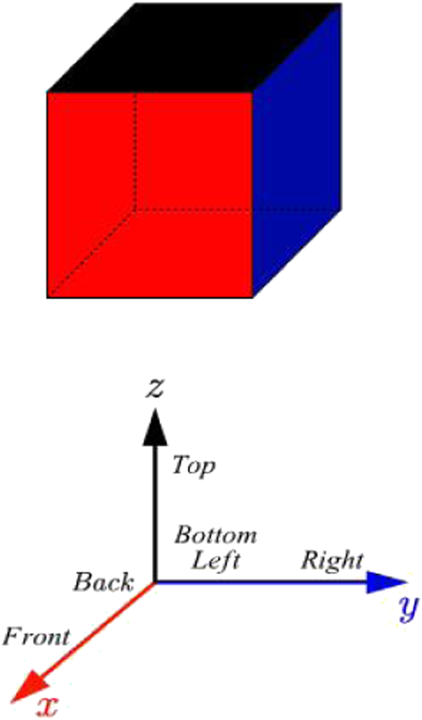
This study used the Easypbc plugin³⁵ to calculate the E11 elastic modulus with periodic boundary conditions, as shown in Figure 11. The equations modeling this system are as follows

X_{F r o n t} - X_{B a c k} = a s s i g n e d v a l u e

(8)

X_{T o p, L e f t} - X_{B o t t o m, R i g h t} = 0

(9)

Y_{T o p,, F r o n t, L e f t} - Y_{B o t t o m, B a c k, R i g h t} = 0

(10)

Z_{F r o n t, T o p, L e f t} - Z_{B a c k, B o t t o m, R i g h t} = 0

(11)where X, Y, and Z represent the displacements of the RVE model along the three directions, respectively. The established RVE model is divided into six faces (i.e., front and back, left and right, and top and bottom). The corresponding mesh nodes on the six faces obey the constraints of the above four equations. Homogenization was used to calculate the equivalent modulus of the composite material via multiple equations.

Figure 11.

Easypbc periodic boundary condition.³⁵

Analysis and results

The equivalent elastic moduli in all simulation models were calculated using Easypbc and summarized in Table 4. For comparison, another correction algorithm, the Modified NNA¹⁷ was used. The experimental results²² are presented in Table 4.

Table 4.

Predicted mean values of effective elastic properties.

Properties	E₁₁(GPa)	E₂₂(GPa)	G₁₂(GPa)	$ν_{12}$	$ν_{23}$
Experiment²²	138	11	5.5	0.28	0.4
RSE (error in %)	138.730 (0.529%)	9.520 (15.506%)	5.133 (7.143%)	0.286 (2.212%)	0.420 (4.762%)
RSE_stirring (error in %)	138.300 (0.217%)	9.640 (12.364%)	5.162 (6.145%)	0.286 (2.212%)	0.420 (4.762%)
Modified NNA¹⁷ (error in %)	138.290 (0.2%)	8.220 (25.28%)	4.560 (17.13%)	0.275 (1.88%)	0.325 (18.78%)

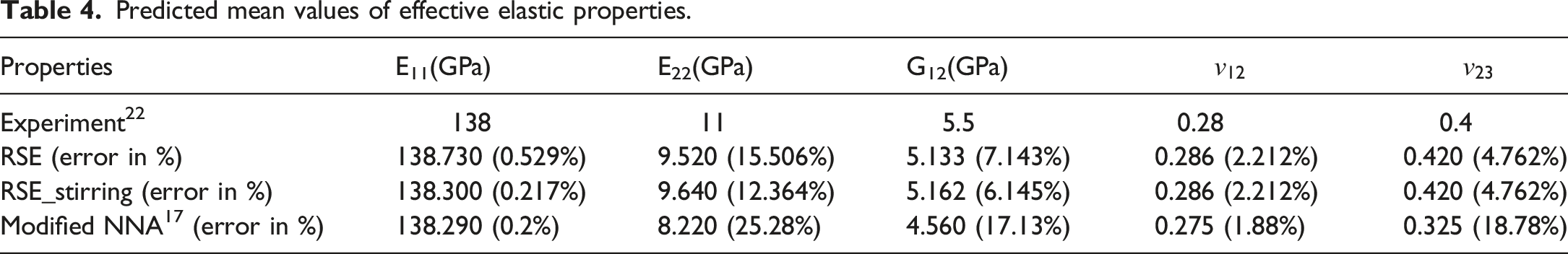
As shown in Table 4, for the Young’s modulus E11 in the main fiber direction, the predicted values of all three algorithms are very close to the experimental results, especially for the two improved algorithms (i.e., RSE_stirring and Modified NNA), which were closer to the experimental values. For the other Young’s and shear moduli, the predicted values of the simulation models were smaller than the experimental ones, which may be attributed to the elimination of interfacial layers between the fibers and the matrix in the actual fiber bundles, as well as the small voids generated inside the matrix during the sample preparation. However, the three algorithms were quite effective in predicting Poisson’s ratio. In general, both the RSE and the RSE_stirring algorithms outperformed the Modified NNA in predicting Poisson’s ratio parameters.

In addition, minor differences were found between the data in Tables 1 and 2 and the simulated data in Table 4. Only five RVE models were used to determine the simulation conditions in each of the first two cases, while 50 RVE models were used for the latter simulation predictions to increase the accuracy of the results.

In general, the RSE_stirring algorithm was optimized from the original RSE algorithm in terms of prediction modulus. Further, the RSE_stirring algorithm with specific stirring was better than the Modified NNA, which was also optimized according to the base algorithm.

Conclusion

In this study, a new algorithm, the RSE_stirring, was proposed to generate random spatial distributions of fibers. This algorithm has two major advantages over the original version of RSE. First, the simulation time required to build each RVE model was less than 3 min, which was significantly faster than the other modeling algorithms. Second, no expensive techniques, such as electron microscopy and image processing, were needed. Further, when considering a stirring step based on the original algorithm, which highlights the influence of fiber short-range spacing interactions, improves the long-range spacing fibers cluster, and the fiber drift phenomenon, the RSE_stirring algorithm is more effective in capturing real fiber distribution.

In terms of statistical analysis, the RVE model, generated by the algorithm, was previously described. Compared with the experimental results, the RSE_stirring algorithms were more consistent with the nearest neighbor distance, the nearest neighbor direction, Ripley’s K function, and the pair distribution function. For the completely random CSR model, the statistical curves of the RSE and RSE_stirring algorithms do not match perfectly, suggesting that the real fiber distribution was not completely random and depended heavily on the manufacturing and the processing conditions.

In summary, the RSE_stirring algorithm is simple, efficient, and can better reproduce the fiber distribution of high-content carbon fiber composites. In addition, the RSE_stirring algorithm facilitates prediction of an equivalent model for simulation.

Footnotes

Declaration of conflicting interests

The author(s) declared no potential conflicts of interest with respect to the research, authorship, and/or publication of this article.

Funding

The author(s) disclosed receipt of the following financial support for the research, authorship, and/or publication of this article: This work was supported by the National Natural Science Foundation of China (U21A20132), Guangxi Specially-invited Experts Foundation of Guangxi Zhuang Autonomous Region.

Data availability

The datasets generated during and/or analyzed during the current study are available from the corresponding author on reasonable request.

ORCID iD

Yibo Li

References

Zheng

Zhang

, et al. Recent advances of interphases in carbon fiber-reinforced polymer composites: a review. Compos B: Eng 2022; 233: 109639.

Chao

Tian

, et al. Numerical evaluation of the influence of porosity on bending properties of 2D carbon/carbon composites. Compos B: Eng 2018; 136: 72–80.

Sun

C T

Vaidya

R S

. Prediction of composite properties from a representative volume element. Compos Sci Technol 1996; 56: 171–179.

Aghdam

M Smith

J Pavier

J . Finite element micromechanical modelling of yield and collapse behaviour of metal matrix composites. J Mech Phys Solids 2000; 48(3): 499–528.

Zhang

Yan

. A comparison between random model and periodic model for fiber-reinforced composites based on a new method for generating fiber distributions. Polym Compos 2017; 38(1): 77–86.

Trias

Costa

Mayugo

A , et al. Random models versus periodic models for fibre reinforced composites. Comput Mater Sci 2006; 38(2): 316–324.

Segurado

Llorca

. A numerical approximation to the elastic properties of sphere-reinforced composites. J Mech Phys Solids 2002; 50(10): 2107–2121.

Wongsto

. Micromechanical FE analysis of UD fibre-reinforced composites with fibres distributed at random over the transverse cross-section. Compos. A: Appl. Sci. Manuf 2005; 36: 1246–1266.

Balasubramani

K Zhang

Chowdhury

T , et al. Micro-mechanical analysis on random RVE size and shape in multiscale finite element modelling of unidirectional FRP composites. Composite Structures 2022; 282: 115081.

10.

Vaughan

J Mccarthy

T . A combined experimental – numerical approach for generating statistically equivalent fibre distributions for high strength laminated composite materials. Compos Sci Technol 2010; 70: 291–297.

11.

Chao

, et al. The effects of interphase parameters on transverse elastic properties of Carbon–Carbon composites based on FE model. Composite Structures 2021; 268: 113961.

12.

Yang

Yan

Ran

, et al. A new method for generating random fibre distributions for fibre reinforced composites. Compos Sci Technol 2013; 76: 14–20.

13.

Kim

W Lim

H Lee

. Prediction and validation of the transverse mechanical behavior of unidirectional composites considering interfacial debonding through convolutional neural networks. Compos B: Eng 2021; 225: 109314.

14.

Melro

R Camanho

P Pinho

T . Generation of random distribution of fibres in long-fibre reinforced composites. Compos Sci Technol 2008; 68: 2092–2102.

15.

Liu

Chen

Xie

, et al. Micro-flow model with a new algorithm of random fiber distribution over the transverse cross-section. Polym Compos 2020; 41(12): 5006–5015.

16.

Feng

Wang

. An adaptive granular representative volume element model with an evolutionary periodic boundary for hierarchical multiscale analysis. Int. J. Numer. Methods Eng 2021; 122(9): 2239–2253.

17.

Wang

Dai

Zhang

, et al. Micromechanical modeling of fiber-reinforced composites with statistically equivalent random fiber distribution. Materials (Basel) 2016; 9(8): 624.

18.

Liu

Zeng

, et al. Development of RVE-embedded solid elements model for predicting effective elastic constants of discontinuous fiber reinforced composites. Mech Mater 2016; 93: 109–123.

19.

Yarlagadda

Deitzel

Heider

, et al. Tailorable universal feedstock for forming (TUFF): overview and performance. Charlotte, NC: SAMPE 2019, 2019.

20.

Heider

Tierney

Henchir

, et al. Microstructural evaluation of aligned, short fiber TuFF material. Charlotte, NC: SAMPE 2019, 2019.

21.

Romanov

Lomov

V Swolfs

, et al. Statistical analysis of real and simulated fibre arrangements in unidirectional composites. Compos Sci Technol 2013; 87: 126–134.

22.

Soden

P D

Hinton

M J

Kaddour

A S

, et al. Lamina properties, lay-up configurations and loading conditions for a range of fibre-reinforced composite laminates. Compos Sci Technol 1998; 58: 1011–1022.

23.

Sun

Zhou

Meng

, et al. An integrated computational materials engineering framework to analyze the failure behaviors of carbon fiber reinforced polymer composites for lightweight vehicle applications. Ecotoxicol Environ Saf 2022; 202: 108560.

24.

Zhang

, et al. Nano-analysis on the structure and chemical composition of the interphase region in carbon fiber composite. Composites Part A: Applied Science and Manufacturing 2014; 56: 143–149.

25.

Sun

Meng

Zhou

Lin

S-P

Kang

Kenten

Guo

. Multi-scale computational analysis of unidirectional carbon fiber reinforced polymer composites under various loading conditions. Composite Structures 2018; 196: 30–43.

26.

Liu Z Zhu P , et al. Generation of random fiber distributions for unidirectional fiber reinforced composites based on particle swarm optimizer. Polymer Composites 2019; 40(4): 1643–1653.

27.

Mehdikhani

Gorbatikh

Verpoest

, et al. Voids in fiber-reinforced polymer composites: A review on their formation, characteristics, and effects on mechanical performance. J. Compos. Mater 2018; 53: 1579–1669.

28.

Zhang

Heider

Gillespie

John

. “Determination of Void Statistics and Statistical Representative VolumeElements (SRVE) in Carbon Fiber Reinforced Thermoplastic Prepregs”. Journal of Thermoplastic Composite Materials 2017; 30(8): 1103–1119.

29.

Eliasson

Karlsson

Hagnell

M Wennhage

, et al. An experimentally based micromechanical framework exploring effects of void shape on macromechanical properties. Materials 2022; 15(12): 4361.

30.

Diggle

J . Statistical analysis of spatial and spatio-temporal point patterns. New York, NY: CRC Press, 2013.

31.

Trias

Costa

Turon

, et al. Determination of the critical size of a statistical representative volume element (SRVE) for carbon reinforced polymers. Acta Mater 2006; 54(13): 3471–3484.

32.

Pyrz

. Quantitative description of the microstructure of composites. Part I: morphology of unidirectional composite systems. Compos Sci Technol 1994; 50(2): 197–208.

33.

ABAQUS 2016 Analysis User's manual. Providence, RI: Dassault Systemes Corp., 2022. http://130.149.89.49:2080/v2016/index.html(2022). (accessed 14 October 2022).

34.

Xia

Zhou

Yong

, et al. On selection of repeated unit cell model and application of unified periodic boundary conditions in micro-mechanical analysis of composites. International Journal of Solids and Structures 2006; 43(2): 266–278.

35.

Omairey

L Dunning

D Sriramula

. Development of an ABAQUS plugin tool for periodic RVE homogenisation. Eng Comput 2019; 35: 567–577.

36.

Tian

Chao

, et al. Periodic boundary condition and its numerical implementation algorithm for the evaluation of effective mechanical properties of the composites with complicated micro-structures. Compos B: Eng 2019; 162: 1–10.

A novel method for generating random fiber distributions for fiber-reinforced materials

Abstract

Keywords

Introduction

Development of algorithm

Statistical characterization

Nearest neighbor distance

Nearest neighbor orientation

Ripley’s K function

Pair distribution function

Prediction of elastic properties

Finite element model

Periodic boundary condition

Analysis and results

Conclusion

Footnotes

Declaration of conflicting interests

Funding

Data availability

ORCID iD

References