Sage Journals: Discover world-class research

Abstract

In-situ manufacturing of thermoplastic composites using the automated fiber placement (AFP) process consists of heating, consolidation and solidification steps. During the heating step using hot gas torch (HGT) as a moving heat source, the incoming tape and the substrate are heated up to a temperature above the melting point of the thermoplastic matrix. The convective heat transfer occurs between the hot gas flow and the composites in which the convective heat transfer coefficient h plays an important role in the heat transfer mechanism which in turn significantly affects temperature distribution along the length, width and through the thickness of the deposited layers. Temperature is the most important process parameter in AFP in-situ consolidation that affects bonding quality, crystallization and consolidation. Although it is well known the convective heat transfer coefficient h is not constant and has a distribution, most studies have assumed a constant value for h for heat transfer analysis which leads to discrepancy between numerical and experimental results. In this study a new function is proposed to approximate the distribution of the convective heat transfer coefficient h in the vicinity of the nip point. Using the proposed convective heat transfer coefficient distribution, a three-dimensional finite element transient heat transfer analysis is performed to predict temperature distribution in the composite parts. An optimization loop is employed to find the free parameters of the distribution function so that the predicted temperature match experimental data. It is shown that, unlike other studies assuming constant h value, not only maximum temperature can be well predicted, but also predicted heating and cooling curves agree well with experimental results. The cooling rate is of significant importance in crystallization behavior and residual stress calculation.

Keywords

Convective heat transfer coefficient heat transfer analysis automated fiber placement thermoplastic composites hot gas torch (HGT)

Introduction

With increasing use of composites in aircraft and automotive structures, automated composite manufacturing techniques have become essential and are attracting much interest from industry. In particular, the automated fiber placement (AFP) process provides a new approach to the manufacturing of large-scale complex composite structures in comparison to traditional manufacturing techniques. It has many advantages such as fast rate of material deposition, reducing materials waste, repeatability in lamination process, reliability etc. With its unique capability to steer narrow tape during layup, AFP has many potentials in manufacturing of high-performance structural components.^1–5

AFP is a process in which composite tapes are laid onto a tool surface in a layer-by-layer manner. During the AFP process an incoming composite tape and certain area of the substrate are heated using a heat source and pressure is applied using a compaction roller to bond the composite tape to the substrate (Figure 1).^1,6,7

AFP can be used in manufacturing both thermoset and thermoplastic composites. Thermoplastic composites, in comparison with thermoset composites, are of special interest due to their superior properties, especially with regard to fatigue and impact issues, infinite shelf life, weldability, toughness, chemical resistance etc. A unique advantage of thermoplastic composites is the possibility of in-situ consolidation that can be achieved using the AFP process alone thus avoiding secondary processes such as autoclave treatments which leads to significant manufacturing cost/energy savings.^1,8–10 Over the past few years the AFP process for in-situ consolidation of thermoplastic composites has been continuously improved. However, many quality issues arise due to fast heating and cooling nature of AFP in-situ consolidation process, especially in composite parts with free edges. Among these issues is development of temperature gradient in different direction as a moving heat source passes on the part to deposit martials. This uneven temperature distribution leads to variation in crystallinity, and give rise to formation of residual stress and deformation. In fact, the most important process parameter in AFP in-situ consolidation that affects the quality is temperature. Material properties (density, specific heat capacity, and thermal conductivity), crystallization behavior, and consolidation all depend on temperature.^6,11,12

There are different types of heat source used in AFP machines including hot gas torch (HGT), laser, heat lamp and infrared heating elements. HGT and laser are the two most common heating source used in in-situ consolidation of thermoplastic composites using AFP. Recently, laser-assisted AFP of thermoplastic composites has attracted much interest from industry, mainly due to high energy density, more focused and more effective heating, faster processing rates and better surface finish. Moreover, better bonding quality and consolidation have been reported in some samples made by laser-assisted AFP. For example, a comparative survey of relative inter-laminar strengths vs. placement rate for CF/PEEK composites made by laser-assisted and HGT-assisted AFP are reported in the study of Stokes-Griffin and Compston.¹² However, there are some limitations in using laser heating system; laser cannot be used in manufacturing of glass fiber composites. This is due to the fact that glass fibers do not absorb the laser energy and therefore, glass fiber composites cannot be heated by laser. Moreover, there are safety concerns involved with implementation of laser; where the laser heating system is used, it should be enclosed to prevent operator exposure to the direct and reflected laser beam.^12–14 On the other hand, HGT has been used since 1986 as a heat source for manufacturing thermoplastic composites in many applications.^8,14,15 HGT has some advantages over laser; first it does not have the safety issues coming with the implementation of the laser. Second, HGT provides more distributed and effective heating in joining areas. Third, as it heats both polymer and fibers, it can be used in processing glass-fiber-based composites. Moreover, in comparison with laser, HGT heating system is less sensitive to and less challenging in positioning of the nozzle outlet.¹⁵

Looking at heat transfer mechanisms in AFP process using HGT, heat flux is transferred to the incoming tape and the substrate from HGT through heat convection and then heat diffuses inside the composites in all three directions (length, width and thickness directions) through heat conduction. Furthermore, the laid-up layers are subjected to the surrounding ambient temperature which cools down the layers. The convective heat transfer is modeled by the Newton’s law of cooling as $q ″ = h_{H G T} (Δ T)$ , where $q ″$ is the heat flux (energy flow per unit of area and time), $h_{H G T}$ is the convective heat transfer coefficient between the HGT and the composite surface and $Δ T$ is the temperature difference between the two media.^16–18 As can be seen from this equation, the convective heat transfer coefficient $h_{H G T}$ plays a significant role in determination of amount of heat that is being transferred to the composites through the hot gas flow generated by HGT. Therefore, the first step in heat transfer analysis of AFP using HGT is to determine the convective heat transfer coefficient $h_{H G T}$ . It is well-known from impinging jet studies¹⁹ and computational fluid dynamics (CFD) simulations²⁰ that the convective heat transfer coefficient $h_{H G T}$ has an extremely non-uniform distribution in the vicinity of the nip point. Despite of this fact, most of studies performed on heat transfer analysis of AFP using HGT assume a constant uniform distribution for $h_{H G T}$ over the heating length for simplicity. This simplifying assumption leads to discrepancy between the predicted temperature distribution and experimental one, especially in heating and cooling rates.

Figure 1.

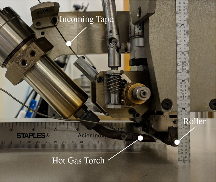
Thermoplastic automated fiber placement head.

Sonmez and Hahn²¹ modeled heat transfer and crystallization of thermoplastic composite tape placement process and investigated the effect of different process parameters. They assumed a constant convective heat transfer coefficient h of $2500 {W/(m}^{2} K)$ in their study. Tierney and Gillespie²² modeled heat transfer and void dynamics for the thermoplastic composite tow-placement process. They obtain the convective heat transfer coefficient h using forced jet-impingement theories. In their study h was assumed to be constant, but no particular value was reported. Toso et al.²³ studied transient three-dimensional (3D) thermal phenomena in thermoplastic tape winding process. They measured the temperature of the incoming tape and the substrate in a static position with an infrared camera. The convective heat transfer coefficient is assumed to be constant and estimated to be around $80 - 100 {W/(m}^{2} K)$ for both the incoming tape and the substrate. A 3D heat analysis for thermoset composite fiber placement process was developed by Hassan et al.²⁴ using finite element (FE) technique. Their solution is based on Lagrangian formulation to solve the transient heat transfer problem which is normally simplified into steady state or quasi-steady state conditions. They included heat generation because of exothermic chemical reactions that occur during curing of thermoset resin in their study. For verification of the FE simulation, composite rings were fabricated using a filament winding machine and temperature was measure using thermocouples. They found a constant value of h coefficient to be $350 {W/(m}^{2} K)$ for the filament winding process.²⁴ Using impinging jet theories, Kim Hee et al.²⁵ calculated the h coefficient to be $900 {W/(m}^{2} K)$ in the vicinity of the nip point and to be $250 {W/(m}^{2} K)$ for the incoming tape. They assumed these values to be constant over the heating length in this study. In 2004, the same authors found the distribution of heat transfer coefficient h along the surfaces of the composite using a coupled 3D flow analysis and two-dimensional (2D) heat conduction analysis via FE technique.²⁰ The heat transfer coefficient has the maximum value of $500 {W/(m}^{2} K)$ right before the nip point in that study. However, the values obtained in their study were only valid for the process parameters considered in that specific AFP setup. Moreover, the calculation of h distribution involved complex 3D flow analysis. In 2015, Li et al.,²⁶ used FE technique to obtain the temperature field in thermoplastic composite tape layup process. The h coefficient values were within the range of $920 - 950 {W/(m}^{2} K)$ and used as an input to their 2D FE model. The 2D FE results were compared with analytical solution of one-dimensional (1D) heat conduction differential equation.

Several researchers^{15,24,27–29} have used an experimental method to determine the h coefficient in which the temperature distribution is measured experimentally (often using embedded thermocouple) and then the value of h coefficient is found in an iterative process so that the maximum temperature predicted by thermal analysis matches the maximum experimental temperature. However, all studies so far using this technique to estimate h coefficient assume a uniform distribution (constant value) for h and only match the maximum temperature obtained experimentally (not the whole temperature distribution including heating and cooling sections). Using this technique, the convective heat transfer coefficient h to be in a range of $180 - 280 {W/(m}^{2} K)$ for a variety of gas volumes for AFP of thermoplastic composites using HGT.²⁸ Temperatures were measured experimentally using the embedded thermocouples and predicted numerically through a 1D heat transfer model through the thickness of the composite laminate. They assumed uniform distribution for h in their study. Recently, Tafreshi¹⁵ investigated the temperature distribution due to the moving HGT in AFP of thermoplastic composites. Using 2D finite difference technique, the temperature gradient were obtained along the layup and through the thickness directions. In order to estimate the convective heat transfer coefficient h, temperature was measured experimentally using fast-response K-type thermocouples through the thickness of the laminate. The convective heat transfer coefficient h was found through an iterative process so that the maximum experimentally measured temperature matches the predicted one. However, h was assumed to be constant (uniform distribution with value of $h = 990 {W/(m}^{2} K)$ along the heating length in their simulation). Consequently, although the maximum predicted temperature agreed well with the experimental one, the rate of temperature change over time (heating and cooling rate) did not agree with experimental results. In 2020, the same authors²⁹ investigated the effect of AFP process parameters on the convective heat transfer h using the above-mentioned semi-experimental-numerical method and impinging jet calculations. On one hand, the 2D finite difference code developed by Tafreshi et al.²⁹ in combination with experimentally measured temperature was used to calculate h for various nozzle temperatures, gas flow rates and nozzle to substrate spacings. On the other hand, h was calculated based on impinging jet heat transfer calculation and determination of Nusselt and Reynolds numbers. Again, a uniform distribution was considered for h in the simulation.

Most studies to date have assumed a uniform distribution for the convective heat transfer h of HGT in the AFP process. As it was shown in previous studies,^15,24 this simplified assumption leads to discrepancy between the experimentally measured temperature and numerically predicted temperature, especially when it comes to heating and cooling portions of the temperature distribution. This means that cooling rate, which has a significant effect on crystallinity of the thermoplastics and residual stress formation in in-situ consolidation of thermoplastic composites using HGT-assisted AFP, cannot be accurately predicted if uniform distribution (i.e., constant value) is assumed for the convective heat transfer h of HGT in the vicinity of the nip point.

In this study, a 3D distribution function is proposed to estimate the convective heat transfer coefficient h of HGT-assisted AFP process. Using the proposed distribution function for h, a 3D transient heat transfer analysis is performed through FE analysis considering moving HGT as a heat source. It is shown that the heating and cooling portions of temperature distribution can be accurately predicted using the proposed h distribution and results agree well with experimental ones. The parameters in the proposed distribution function for h may be determined based on experimentally measured temperature for different AFP configurations to accurately predict not only maximum temperature, but also heating and cooling rates.

AFP HGT convective heat transfer coefficient distribution

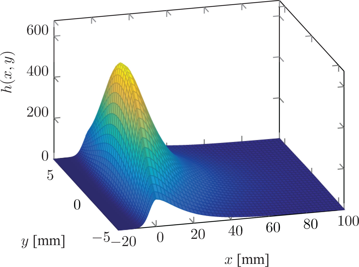
Previous studies have shown that the convective heat transfer coefficient h has a significant influence on the temperature distribution during the AFP process and is dependent on various number of parameters such as nozzle geometry, gas flow rate, nozzle temperature and type of the gas etc. Accurate prediction of the temperature distribution within the laminate is mandatory to subsequently calculate stresses and displacements properly. Therefore, for heat transfer analysis and/or thermo-mechanical analysis, it is important that h distribution can be described as accurately as possible by a function. Kim et al.²⁰ estimate the distribution of the heat transfer coefficient during the HGT-assisted AFP process along the surfaces of the composite via a three-dimensional flow analysis and two-dimensional heat transfer analysis for a specific machine configuration using finite element method (FEM). It was shown that h has an unsymmetrical distribution, sharply rises in the vicinity of the nip point (with maximum value at the stagnation point) and falls more gradually after the stagnation point. Similar distribution of h is also observed from impinging jet calculation for an inclined torch impinging the surface at an angle.¹⁹ These results are the basis for the new proposed distribution function for the heat transfer coefficient h of HGT-assisted AFP process. The proposed distribution function is plotted in Figure 2 in which x is the layup direction (moving direction of the HGT) and y is along the width direction. The steep rise in the x direction (Figure 2(b)) is explained by the fact that the HGT is inclined and the hot gas is blocked by the roller at the nip point and therefore the stagnation point, where h is peaked, is slightly distanced from the nip point. After the peak the decline in h value is more gradual compare to the sharp rise before the peak. It can be seen that the distribution function for the heat transfer coefficient h has three parts: left shoulder, peak and right shoulder. While the distribution of h is unsymmetrical along the layup direction x, along the width, h has a symmetrical distribution as shown in Figure 2(c).

Figure 2.

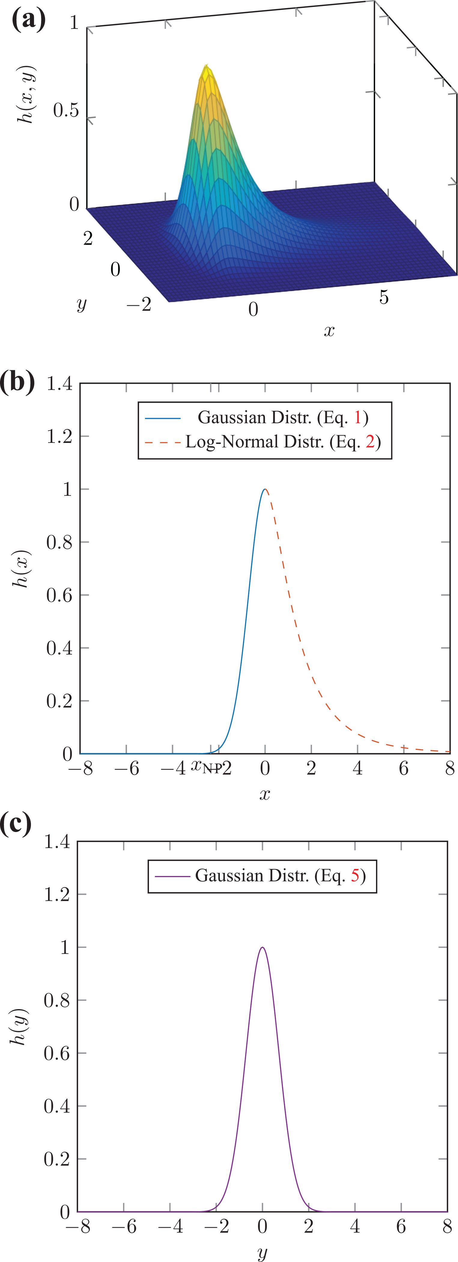
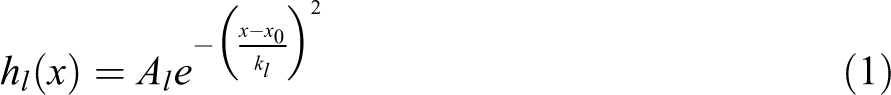
Distribution function for the convective heat transfer coefficient h. The peak position is at $x_{0} = 0$ and $y_{0} = 0$ . $A = k_{l} = k_{r} = k_{y} = 1$ , $x_{N P} = nip point$ . (a) 3D distribution, (b) 2D distribution in x direction and y = 0, and (c) 2D distribution in y direction and x = 0.

In our approach to approximate the convective heat transfer coefficient h, a two-variable distribution function is defined in which the value of h is a function of x and y coordinates. The moving direction of the HGT is denoted by x (layup direction), and the direction perpendicular to it by y along the width of the tape. Two different functions are used to approximate the distribution of the h coefficient. Two base functions are used to estimate unsymmetrical nature of h distribution in the x direction and the symmetrical h distribution in the y direction. The first base function is a Gaussian normal distribution in the form of equation (1) which is inspired by metal welding process simulations.³⁰ This function contains three free parameters needed to be determined. A_l determines the magnitude of the peak while the parameter k_l is a concentration coefficient and defines the slope of the curve. The index l represents “left,” because the function g_l approximates the h distribution on the left side of the peak. The variable x₀ determines the location of the peak in the x direction.

h_{l} (x) = A_{l} e^{- {(\frac{x - x_{0}}{k_{l}})}^{2}}

The Gaussian distribution tends quickly toward zero and thus is not suitable to represent the unsymmetrical distribution characteristics of the h coefficient, especially in the right shoulder. Therefore, a second function which is a modified log-normal distribution function, equation (2), is proposed for the right branch (i.e., upstream region).

h_{r} (x) = A_{r} e^{- ln ({(\frac{r (x)}{k_{r}} + 1)}^{2})}

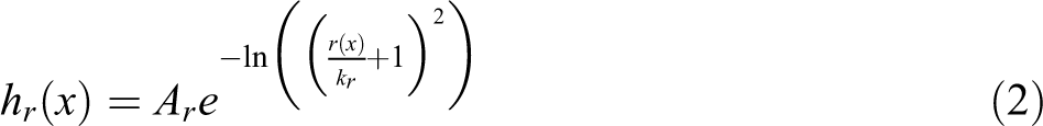
In this function, r is the distance between the variable x and the location of the peak located at x₀ and is defined by Euclidean norm (equation (3)), k_r is a concentration coefficient and the index r represents “right” branch. The result is a symmetrical distribution, which is also defined in the negative number range. In Figure 2(b), this modified log-normal distribution is plotted together with the Gaussian normal distribution. The modified log-normal distribution function has a flatter slope compare to the Gaussian normal distribution function.

r (x) = ∥ x - x_{0} ∥_{2}

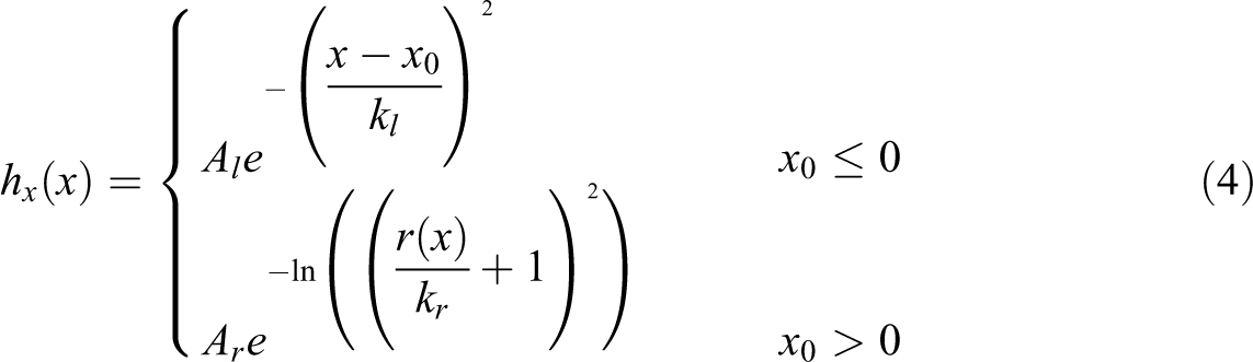
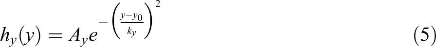
If the amplitudes A_l and A_r are assumed to be equal, a continuous piecewise function can be constructed from equations (1) and (2), as shown in equation (4). The gradient of the equations (1) and (2) is zero at the position of the peak (i.e., $x = x_{0}$ ), thus, ensuring continuity for the proposed function (i.e., equation (4)).

h_{x} (x) = \{\begin{array}{l} A_{l} e^{- {(\frac{x - x_{0}}{k_{l}})}^{2}} & x_{0} \leq 0 \\ A_{r} e^{- ln ({(\frac{r (x)}{k_{r}} + 1)}^{2})} & x_{0} > 0 \end{array}

For the distribution of the convective heat transfer coefficient h in the width direction of the tape, a function dependent on the variable y is needed. For this the variables x and x₀ in equation (1) are exchanged with y and y₀.

h_{y} (y) = A_{y} e^{- {(\frac{y - y_{0}}{k_{y}})}^{2}}

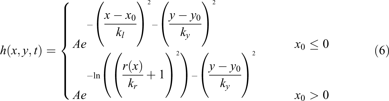
Finally, a combination of the two introduced distribution functions (equations (4) and (5)) is used to propose the distribution of the heat transfer coefficient $h (x, y)$ which is a two-variable function depending on the two coordinates x and y. This can be achieved by multiplying the distribution functions in x and y directions (equation (4) and equation (5), respectively) and by assuming the same amplitudes ( $A = A_{l} = A_{r} = A_{y}$ ) for all functions as shown in equation (6).

h (x, y, t) = \{\begin{array}{l} A e^{- {(\frac{x - x_{0}}{k_{l}})}^{2} - {(\frac{y - y_{0}}{k_{y}})}^{2}} & x_{0} \leq 0 \\ A e^{- ln ({(\frac{r (x)}{k_{r}} + 1)}^{2}) - {(\frac{y - y_{0}}{k_{y}})}^{2}} & x_{0} > 0 \end{array}

This function has a peak that is defined by the variable x₀ and y₀. The moving heat source (hot gas torch) is mounted on the robot head and moves at a constant speed v in the x direction. This means that the position of the peak at x₀ and thus the whole distribution function $h (x, y)$ moves at the same speed v and therefore is a function of time t. Knowing the speed of the moving heat source v, the position x₀ can be calculated as

x_{0} = x_{0} (t) = x_{t_{0}} + t \cdot v

where $x_{t_{0}}$ is the initial position of the moving heat source peak at t₀.

The proposed HGT convective heat transfer coefficient distribution, equation (6), has four parameters, namely A, k_l, k_r and k_y, needed to be determined for any AFP configuration based on matching experimentally measured temperature with the predicted one via FE analysis. This parameter fitting procedure is explained in the following sections.

Parameter fitting

Determination of parameters A, k_l, k_r and k_y in HGT convective heat transfer coefficient distribution $h (x, y)$ consists of measuring experimentally the temperature of the laminate during AFP process, performing heat transfer analysis using FE method (or other techniques like finite difference method) and determining the four aforementioned parameters through an optimization routine until the predicted temperature found via analysis agrees with the experimental one. For this purpose, a residual function is defined as the objective function which is the difference between the temperature distribution measured experimentally during the AFP process and predicted via FE transient heat transfer analysis. In the following the FE model and the underlying experiment are described in more details, followed by the fitting procedure to obtain h distribution’s parameters

FE model

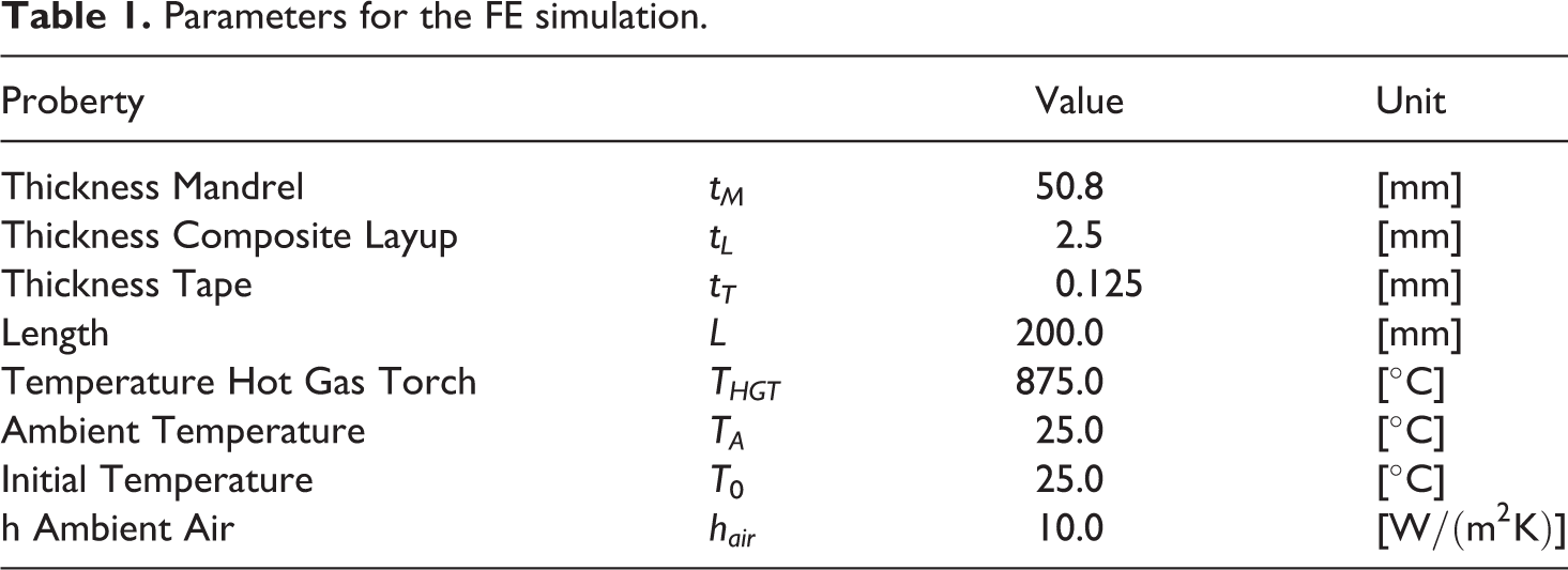
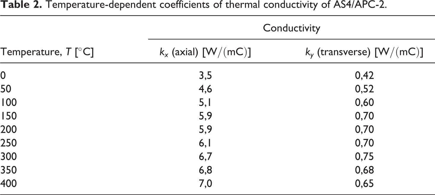
For thermal analysis via FEM, Abaqus solver 2016 is used. Abaqus FEA is a commercial software package that solves problems of solid-state statics and dynamics, heat conduction, electromagnetism and fluid dynamics. A 3D FE model is developed in which the HGT is modeled as a convective moving heat source. The schematic model is shown in Figure 3 and geometrical parameters along with material properties and model parameters are listed in Table 1. The dependency of the coefficients of thermal conductivity on temperature and direction are considered in the analysis (temperature-dependent properties are listed in Table 2). The “DC3D20” element, a 3D 20-node quadratic isoparametric element for heat transfer is used from the Abaqus element library for meshing both composite layers and aluminum tool. The model is divided into two regions: the composite layers and the mandrel. Mesh convergence analysis was performed by reducing the element size of the mesh until the temperature did not change within ±1°C. The final element size of the composite layers in both x and y directions is 0.6 mm and in z direction the element size is 0.0625 mm. The size of the elements of the mandrel in x and y direction is the same as the composite layers, however, along the thickness direction (z) the model is built based on adaptive mesh strategy in which the mesh refinement is applied from the mandrel region toward the top composite layer (Figure 4). This way one can take advantage of the fact that thermal gradients are attenuated from the top layer toward the mandrel. Attention is paid to the fact that there should be a node at the respective position of the thermocouple under the first composite layer measuring the temperature experimentally. A transient thermal analysis is performed using Abaqus Standard Solver. The temperature is calculated for each time step on the position of the thermocouple. Thus, a thermal profile can be determined as a function of time. 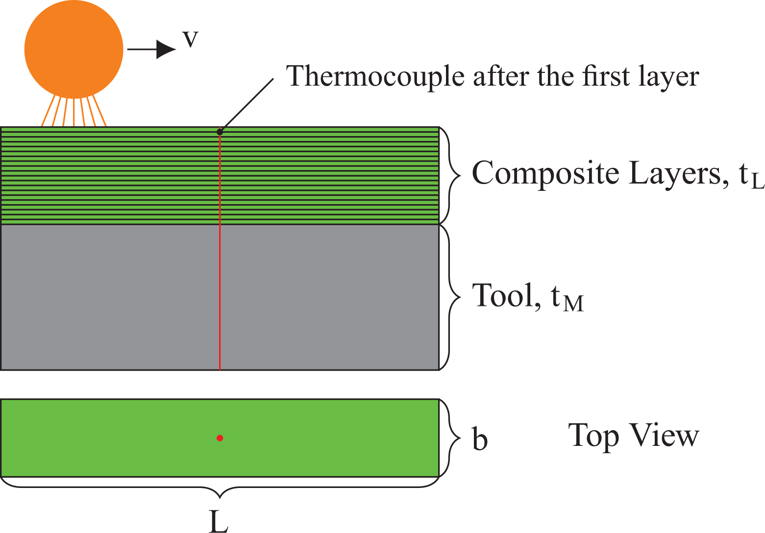The heat flux of the moving heat source (HGT) through the upper surface of the composite layup is calculated using the proposed convective heat transfer coefficient distribution $h (x, y)$ as per equation (6) and implemented with a DFLUX user-subroutine in Abaqus. A Python script is used to generate the model in Abaqus/CAE. The advantage of using a Python script to generate the model is that a fully parameterized model can be created and the parameters can be controlled via a Matlab script for optimization routine which is explain in following sections.

Figure 3.

Schematic illustration of the composite laminate with embedded thermocouples, the aluminum mandrel and 20 tapes.

Table 1.

Parameters for the FE simulation.

Proberty		Value	Unit
Thickness Mandrel	t_M	50.8	[ $mm$ ]
Thickness Composite Layup	t_L	2.5	[ $mm$ ]
Thickness Tape	t_T	0.125	[ $mm$ ]
Length	L	200.0	[ $mm$ ]
Temperature Hot Gas Torch	$T_{H G T}$	875.0	[°C]
Ambient Temperature	T_A	25.0	[°C]
Initial Temperature	T ₀	25.0	[°C]
h Ambient Air	$h_{a i r}$	10.0	[ ${W/(m}^{2} K)$ ]

Table 2.

Temperature-dependent coefficients of thermal conductivity of AS4/APC-2.

Temperature, T [°C]	Conductivity
Temperature, T [°C]	k_x (axial) [ $W/(mC)$ ]	k_y (transverse) [ $W/(mC)$ ]
0	3,5	0,42
50	4,6	0,52
100	5,1	0,60
150	5,9	0,70
200	5,9	0,70
250	6,1	0,70
300	6,7	0,75
350	6,8	0,68
400	7,0	0,65

Figure 4.

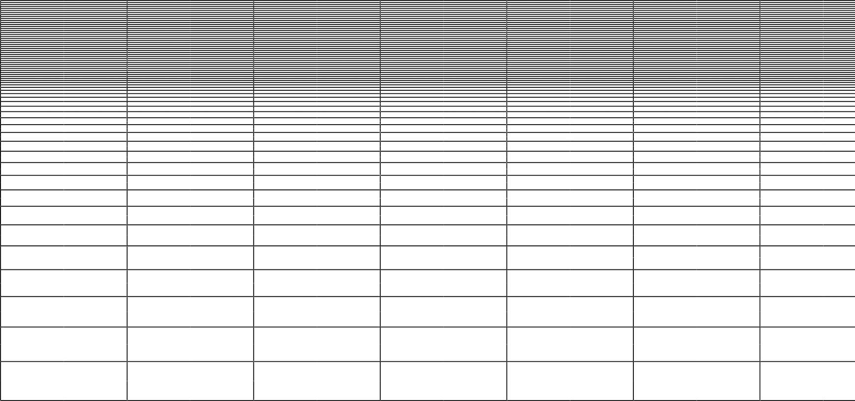
Adaptive mesh through the thickness of the model.

Experiment

To measure the temperature during the HGT-assisted AFP process, flat unidirectional composite strips were made using a robotic-type AFP machine and flat paddle tool available at the Concordia Centre for Composites (CONCOM) shown in Figure 5. The AFP machine is equipped with a HGT system that employs hot nitrogen gas to melt the thermoplastic matrix and a 12.7 mm (0.5 inch) diameter steel roller to consolidate the materials. The samples were made using 6.35 mm (0.25 inch) wide carbon fiber/PEEK (AS4/APC-2) tape supplied by Solvay Group. The details of the experiments were described by Tafreshi et al.²⁹ and is briefly summarized here. Thermocouples were embedded between composite layers to measure the thermal profiles through the thickness of the composite unidirectional strip subjected to a moving heat source (HGT). The main focus was on t how temperature gradient develops by time during the AFP process through the thickness of the composite laminate. The test specimen and experimental setup is illustrated in Figure 3. Unidirectional composite strips of 508 mm long making up 20 layers were manufactured on the aluminum mandrel. Temperature measurements recorded using a thermocouple mounted under the first composite layer are used in this study for fitting procedure. Before the temperature measurements begun, the composite body was cooled down to ambient temperature. No materials deposition was done during the temperature measurement trials. 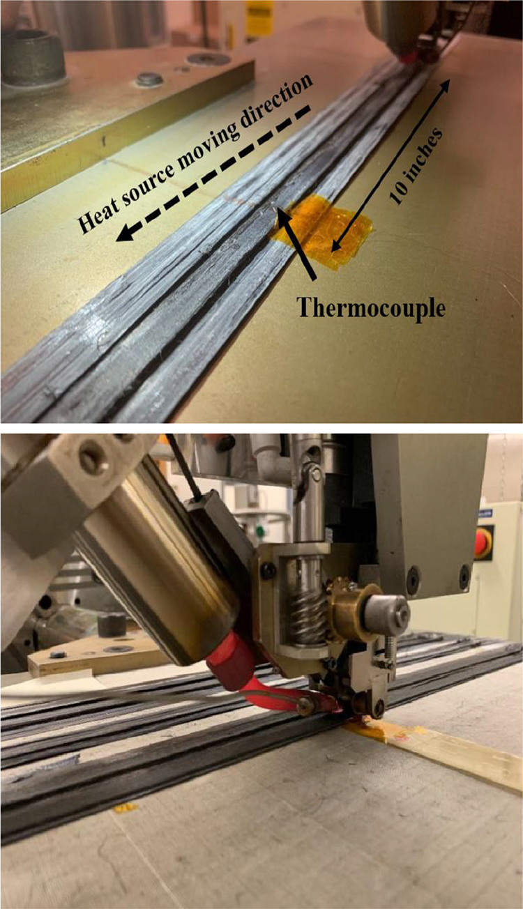The AFP head with the HGT and the roller moves with speed $v = 25.4 mm/s$ along the surface and the HGT temperature was set at 875°C.

Figure 5.

Experimental setup; location of AFP head (left) at the beginning of the pass (right) over the embedded thermocouples.³¹

Fitting procedure

The four parameters (k_l, k_r, k_y and A) for the convective heat transfer coefficient distribution function $h (x, y)$ proposed in equation (6) are fitted with an optimization routine in Matlab based on the simplex search method of Lagarias et al.³² This is a direct search method that does not use numerical or analytic gradients and is appropriate for non-smooth problems. The parameters k_l, k_r, k_y and A from equation (6) are fitted during optimization in such a way that the temperature distribution predicted by FE analysis coincides with that from the experiment.

An optimization with all four parameters at the same time is not recommended, as this proved to be very time-consuming and inefficient. So the optimization process for fitting the parameter is divided into three sub-steps as seen in Figure 6. The fitting procedure presented in Figure 7 is applied for each of the sub-steps. In the first sub-step, the error in the peak is minimized by adjusting the amplitude value A. In the second sub-step, the error on the right side of the peak related to the downstream region is minimized by adjusting the concentration coefficient k_y and k_r. In the third and last sub-step, the left side of the peak related to the upstream region is fitted using the parameter k_l. These three steps can be repeated as often as required until the maximum difference between experiment and FEM is acceptable. In this study, the aforementioned sub-steps are repeated twice and the results of each of three sub-steps are plotted in Figure 8(a) to (d), respectively.

Figure 6.

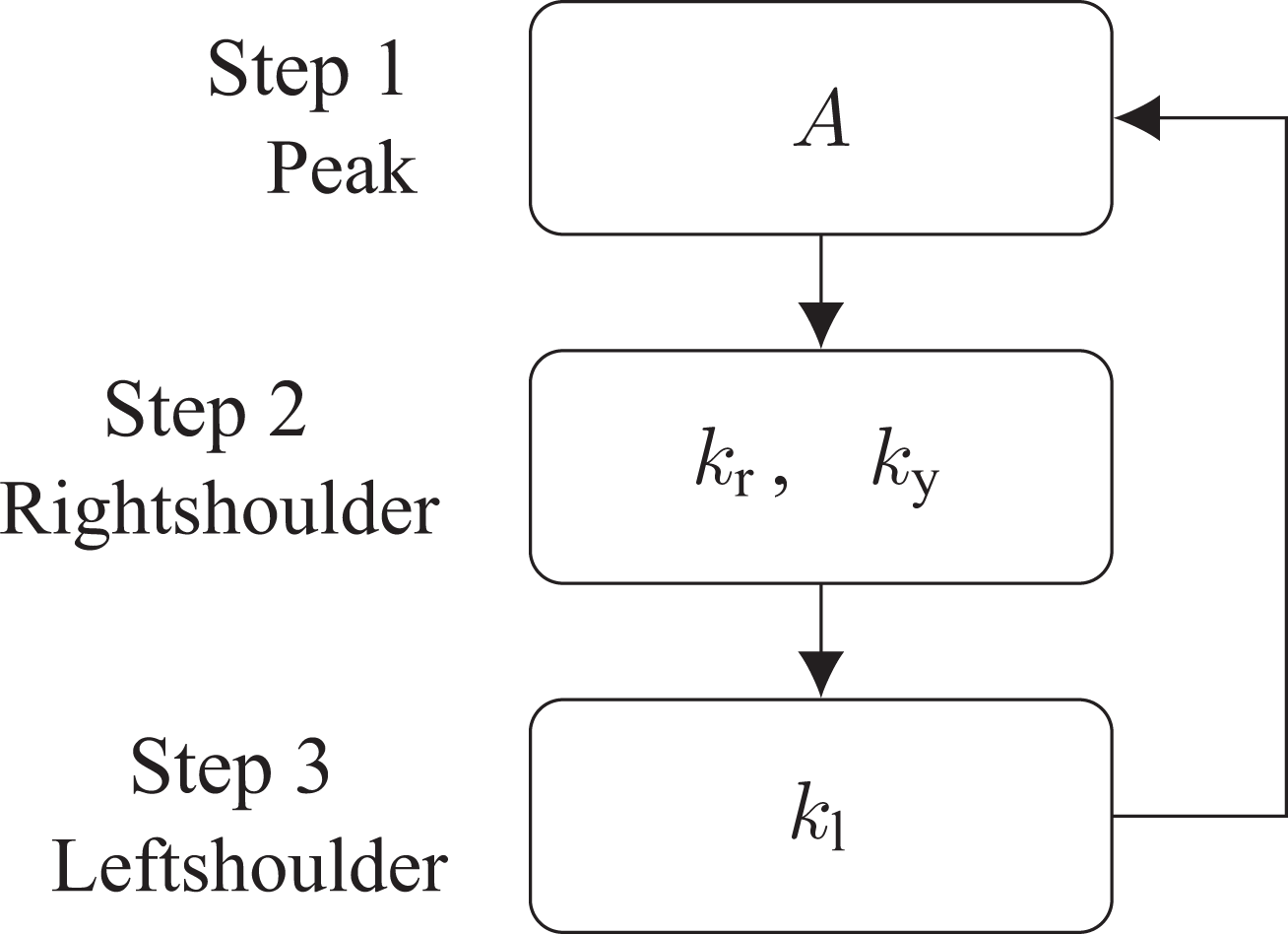
Three sub-steps for fitting the parameter (A, k_l, k_r, k_y).

Figure 7.

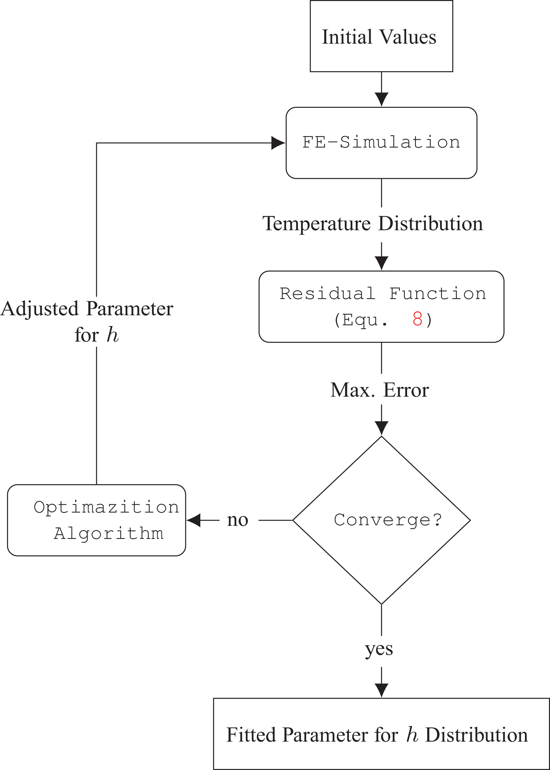
Optimization loop for fitting the free parameters to the experimental result.

Figure 8.

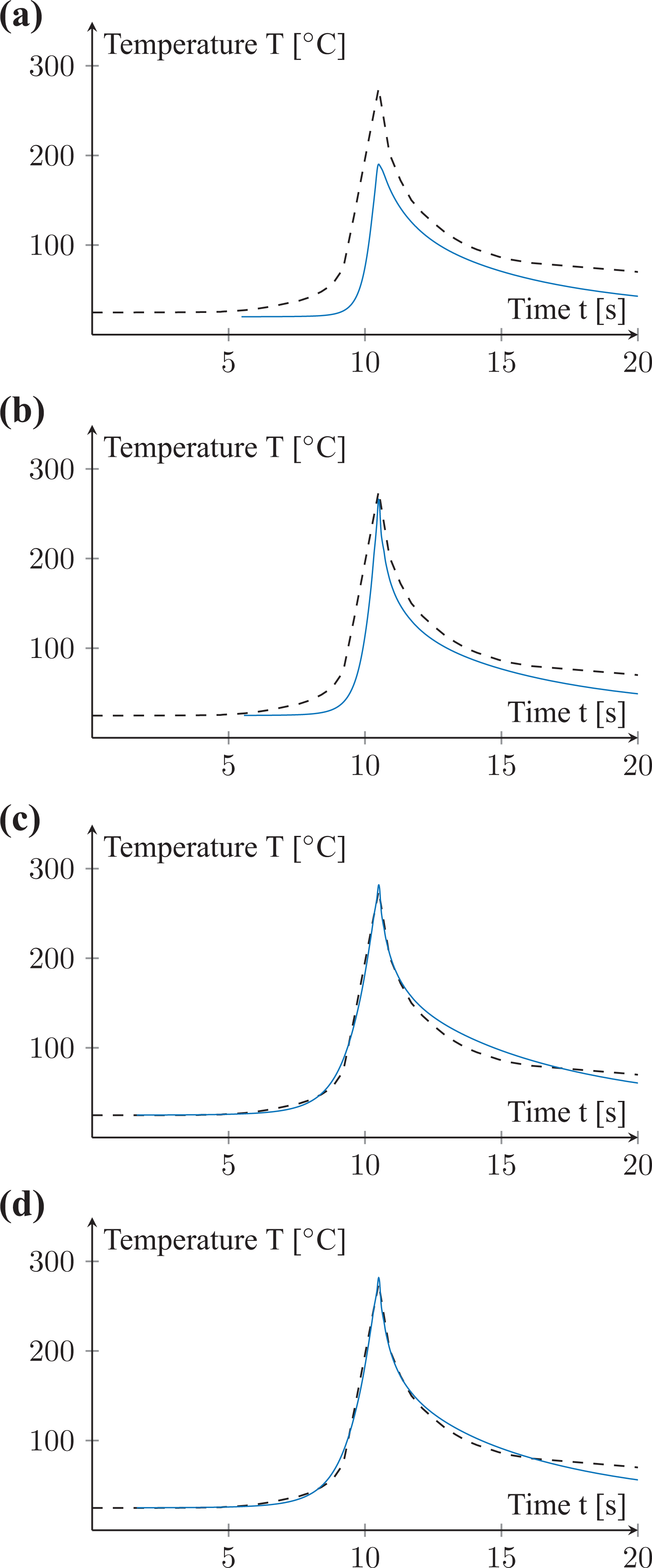
Plots of the temperature over time after the each fitting step. (a) Initial values for the parameter, (b) first step: fitting the temperature peak, (c) second step: fitting the left side of the temperature curve, and (d) third step: fitting the right side of the temperature curve.

The fitting of the process parameters in each of the sub-steps is done by an optimization procedure, which is sketched in Figure 7. As the first step, the temperature distribution is calculated in the FE simulation based on some initial values for the four parameters (i.e. A, k_l, k_r and k_y). Then a residual function defined in equation (8) is considered as the objective function for the optimization problem.

f_{r e s} = max (∥ T^{E x p} - T^{F E M} ∥_{2})

where $∥ \cdot ∥_{2}$ is Euclidean norm. With this residual function the maximum difference between the temperature distribution calculated by experiment and simulation is determined at the position of the sensor (compare Figure 3). Depending on the parameter to be minimized, the maximum difference in one of the three regions of the temperature distribution (peak, left shoulder and right shoulder) is determined (e.g. the peak for fitting the amplitude A etc. see Figure 6). The value of the residual function is minimized by the parameters adjustment of the optimization algorithm. In every loop the adjusted parameter for calculating the $h (x, y)$ distribution passed to the FE solver. This loop is repeated until the value of the residual function converges.

The results from FE simulation and experiment are based on different time steps and do not match with each other. So the two data sets (i.e., FE-predicted and experimentally measured temperature) are sampled at the same N different points throughout the time using linear interpolation.

Results

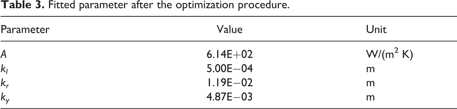
The aforementioned procedure to find the HGT convective heat transfer coefficient distribution $h (x, y)$ is employed to determine the $h (x, y)$ distribution of the HGT used in experiment performed at CONCOM AFP lab as described in the “Experiment” section. The final results of the fitting procedure (i.e., the values of A, k_l, k_r and k_y) are listed in Table 3 and $h (x, y)$ distribution is plotted in Figure 9. The predicted temperature using this $h (x, y)$ distribution along with experimental results and results predicted by Tafreshi et al.²⁹ is shown in Figure 10. As can be seen, using the proposed h distribution, the predicted temperature is in a very good agreement with the experimental one, not only at peak value, but also during heating and cooling periods. As can be seen, although the simulation result by the same author predicts the peak temperature accurately, there is a large deviation during heating and cooling periods between predicted and experimental temperature. This is due to the fact that Tafreshi et al.²⁹ uses a constant h distribution with a value of $h = 990 {W/(m}^{2} K)$ which cannot capture the heating and cooling period properly. However, using the proposed $h (x, y)$ distribution with a maximum value of $h_{max} = 614 {W/(m}^{2} K)$ as shown in Figure 9, this limitation is overcome and heating rate and cooling rate can be accurately predicted.

Table 3.

Fitted parameter after the optimization procedure.

Parameter	Value	Unit
A	6.14E+02	W/(m² K)
k_l	5.00E−04	m
k_r	1.19E−02	m
k_y	4.87E−03	m

Figure 9.

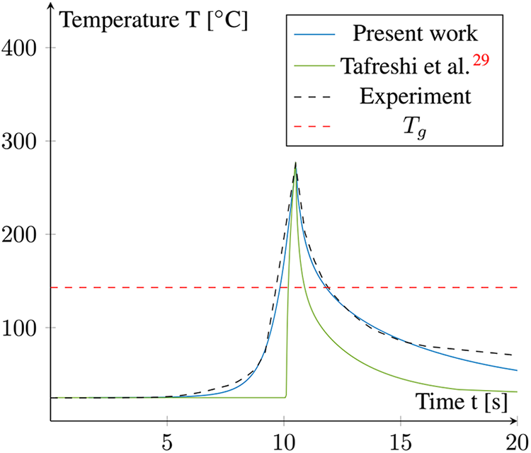
Distribution for $h (x, y)$ from equation (6) after the fitting procedure.

Figure 10.

Comparison between FE simulation and experimental result.

Using the obtained $h (x, y)$ , the temperature distribution in the vicinity of the heat source along the layup direction for different layers through the thickness is shown in Figure 11 and compared with similar results from Tafreshi et al.²⁹ $ξ$ is a transformation on the x-axis showing the distance between the heat source and points of interest along the layup direction ( $ξ = x_{0} - v \cdot t$ where v is the HGT speed and x₀ is the position of the peak of h). Negative $ξ$ ( $ξ < 0$ ) indicates the upstream region where the HGT already passed and heated up the region, while the positive $ξ$ ( $ξ > 0$ ) shows the downstream region. As can be seen from Figure 11 the temperature gradient in downstream region is more than the temperature gradient in upstream region. This is mainly due to the fact that upstream region has been already heated by HGT while the downstream region has not. Comparing the results with those obtained by Tafreshi et al.,²⁹ it can be seen that the temperature gradient predicted by the present study are lower in both upstream and downstream regions compared to the same author (i.e., the predicted temperature is higher in both regions). This difference is because of the different assumptions made for HGT h distribution. While h distribution is assumed to be uniform (constant h value),²⁹ in this study h varies by x and y based on the distribution function shown in Figure 9.

Figure 11.

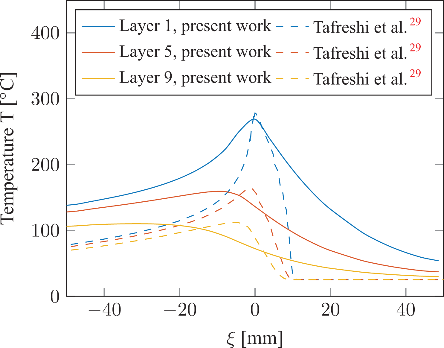
Temperature distribution in the vicinity of the heat source along the layup direction after 1, 5 and 9 layers.

Looking at through-the-thickness temperature distribution, it can be seen that up to five layer below the composite top surface, the peak temperature is above glass transition temperature (T_g). In comparison with results of Tafreshi et al.,²⁹ it can be seen that the area predicted to be above T_g by assuming variable h distribution is bigger. For example, in layer 1, area between −43 mm < x₀ < 24 mm is above T_g, while based on Tafreshi et al.²⁹ prediction, this area is between −5.7 mm < x₀ < 5.7 mm. The areas with the temperature above T_g is of practical importance for repass treatment (reconsolidation pass) which leads to improvement in bonding quality, reduction of void content and improvement of surface finish of in-situ consolidated thermoplastic composites as reported in the literature.^8,28 Furthermore, it can be seen that the peak temperatures for layers below the top surface are shifted more to the left compared to Tafreshi et al.²⁹ This shift is due to the fact that it takes time for the heat provided by HGT to diffuse from the top surface to the layers below and through the thickness of the laminate.

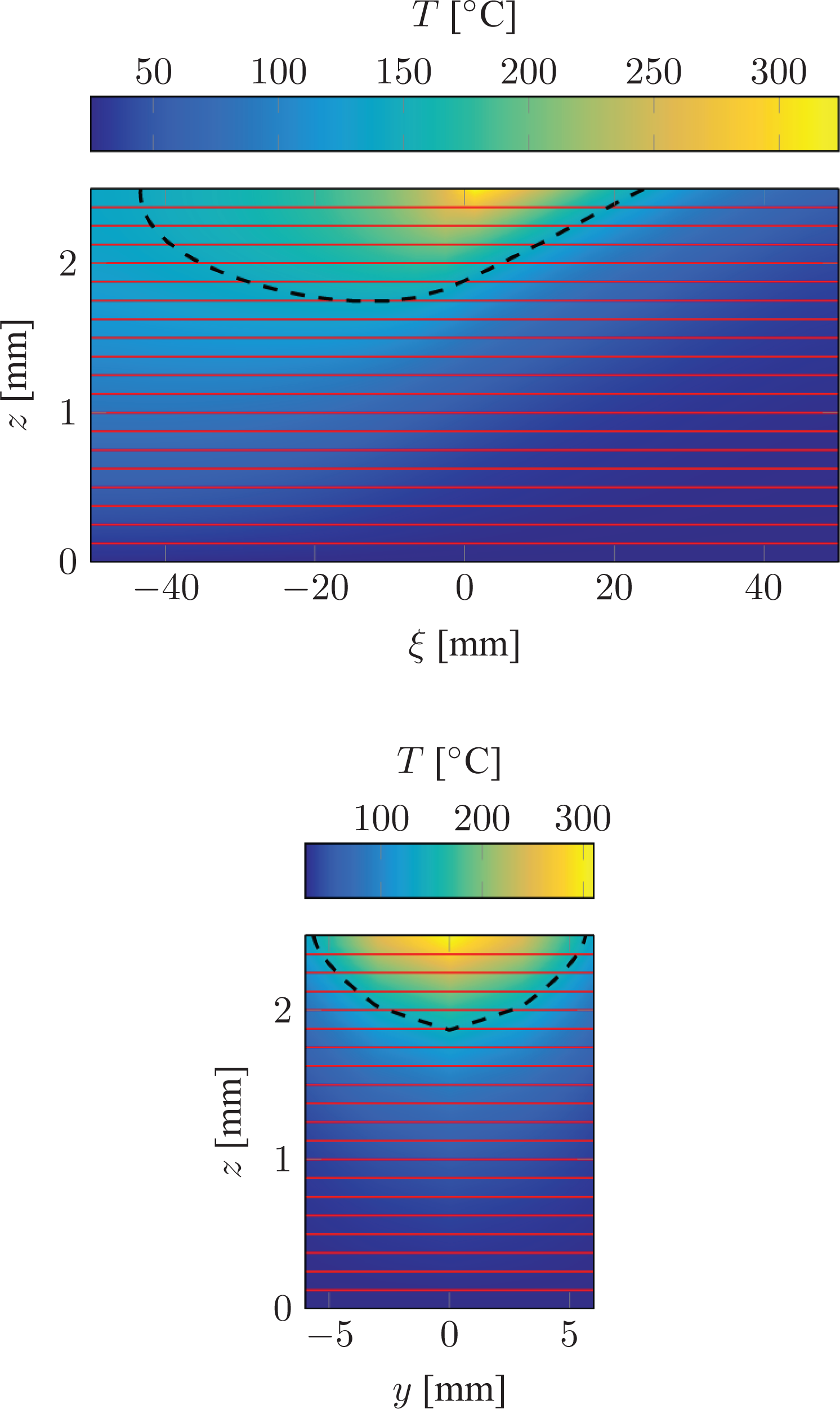
Using the obtained $h (x, y)$ distribution, the temperature contour plot in the vicinity of the heat source along the layup direction, through the thickness and along the width of the tape is plotted in Figure 12, respectively. As expected, the temperature distribution along the width direction is symmetric about the mid point of the tape (Figure 12, right). However, looking at the left contour plot in Figure 12, the temperature gradient is unsymmetrical showing that the upstream region where already heated by HGT is at higher temperature compared to downstream region. The dashed line shows the area of the laminate that is above T_g which has significance in development of residual stress and distortion due to temperature gradient.

Figure 12.

Temperature distribution in the composite layup. The position of peak is at $x = 0$ mm and $y = 0$ mm. The red lines separate the individual layers and the black dashed line show area where temperature is more than 143°C.

Sensitivity study

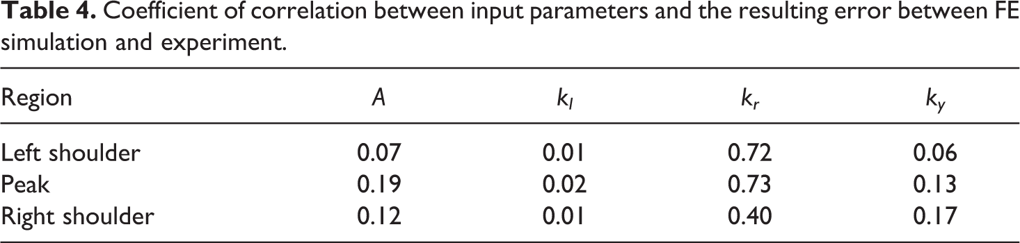
A global sensitivity analysis is employed to determine the coefficient of correlation (CoC) between input parameters, namely A, k_l, k_r and k_y, and the output parameter which is the error between FE simulation and experiment. The CoC is the standardized covariance between two variables measuring the strength and the direction of a relationship between the two variables. If both variables have a strong positive correlation, the CoC is close to 1. For a strong negative correlation the CoC is close to −1. A value close to zero indicates that there is almost no correlation between the two variables under consideration.³³ For the sensitivity analysis, the software optiSLang, developed by Dynardo GmbH, and coupled with the Abaqus solver is used. In a range of $\pm 10 %$ based on the fitted parameter in Table 3 100 samples are generated with the Advanced Latin Hypercube Sampling method.³⁴ The error in one of the three regions of the temperature distribution (peak, left shoulder, right shoulder) is used as the output parameter (i.e., response variable). The result is presented in Table 4. It can be seen that the parameter k_r has the most influence on the response, while the parameter k_l has the least effect. This can be explained by looking at h distribution (Figure 2) and noticing that the right shoulder of the h distribution curve spans longer than the left shoulder. Thus a larger amount of energy can be transferred into the structure. This has more influence in the downstream region and affect the resulting temperature distribution significantly. Furthermore, it is obvious that k_y, which represents the distribution of h in the width direction of the tape, has a non-negligible influence on the result and therefore, the variation of h in both x (along the length) and y (along the width) directions should be considered in the analysis to have an accurate temperature prediction.

Table 4.

Coefficient of correlation between input parameters and the resulting error between FE simulation and experiment.

Region	A	k_l	k_r	k_y
Left shoulder	0.07	0.01	0.72	0.06
Peak	0.19	0.02	0.73	0.13
Right shoulder	0.12	0.01	0.40	0.17

Conclusion

A new distribution piece-wise function is proposed to estimate the distribution of the convective heat transfer coefficient $h (x, y)$ of HGT-assisted AFP process. The four free parameters inside the proposed distribution function may be determined via an optimization loop by matching experimentally measured temperature during AFP process with predicted temperature from heat transfer analysis. Using the proposed convective heat transfer coefficient distribution, a three-dimensional finite element model of AFP process is developed and transient heat transfer analysis considering moving heat source is performed to predict temperature distribution in the composite parts. It is shown that the variation of temperature through time can be accurately predicted by the proposed $h (x, y)$ distribution function and result agrees well with experimental one during heating, at peak and during cooling stage. This overcomes the issues rising from assuming uniform distribution for h which leads to discrepancy between the predicted temperature distribution and experimental one, especially during heating and cooling. The accurate prediction of heating and cooling rates are important especially in studying crystallization behavior and calculating residual stress and deformation of in-situ consolidated thermoplastic composites. For future work, the effect of different process parameters including placement speed, gas flow rate, nozzle temperature etc. on determination of the proposed convective heat transfer coefficient will be studied.

Footnotes

Acknowledgment

Financial support from the Mitacs Canada through Globalink program is appreciated.

Funding

The author(s) disclosed receipt of the following financial support for the research, authorship, and/or publication of this article: This work was supported by Mitacs Canada through Globalink program.

ORCID iD

Klemens Rother

References

Van Hoa

. Principles of the manufacturing of composite materials. 2nd ed. Lancaster, PA: DEStech Publications, Inc., 2018.

McIlhagger

Archer

McIlhagger

. Manufacturing processes for composite materials and components for aerospace applications. In: Polymer composites in the aerospace industry. Woodhead Publishing Series in Composites Science and Engineering, 2020, pp. 59–81.

Clancy

Peeters

Oliveri

, et al. Steering of carbon fiber/thermoplastic pre-preg tapes using laser-assisted tape placement. In: AIAA/ASCE/AHS/ASC structures, structural dynamics, and materials conference, Kissimmee, FL, 8–12 January 2018, p. 478.

Nik

Fayazbakhsh

Pasini

, et al. Optimization of variable stiffness composites with embedded defects induced by automated fiber placement. Compos Struct 2014; 107: 160–166.

Ghasemi Nejhad

. Issues related to processability during the manufacture of thermoplastic composites using on-line consolidation techniques. J Thermoplast Compos Mater 1993; 6: 130–146.

Hoa

Duc Hoang

Simpson

. Manufacturing procedure to make flat thermoplastic composite laminates by automated fibre placement and their mechanical properties. J Thermoplast Compos Mater 2017; 30: 1693–1712.

Aized

Shirinzadeh

. Robotic fiber placement process analysis and optimization using response surface method. J Thermoplast Compos Mater 2011; 55: 393–404.

Shadmehri

Hoa

Fortin-Simpson

, et al. Effect of in situ treatment on the quality of flat thermoplastic composite plates made by automated fiber placement (AFP). Adv Manuf 2018; 4(2): 41–47.

Cogswell

. Thermoplastic aromatic polymer composites—a study of the structure, processing and properties of carbon fibre reinforced polyetheretherketone and related materials. Amsterdam: Elsevier Publication, 2013.

10.

Jeyakodi

. Finite element simulation of the in-situ AFP process for thermoplastic composites using Abaqus. Master’s Thesis, TU Delft, UK, 2016.

11.

Schledjewski

Latrille

. Processing of unidirectional fiber reinforced tapes—fundamentals on the way to a process simulation tool (ProSimFRT). Compos Sci Technol 2003; 63: 2111–2118.

12.

Stokes-Griffin

Compston

. The effect of processing temperature and placement rate on the short beam strength of carbon fibre-PEEK manufactured using a laser tape placement process. Compos A Appl Sci Manuf 2015; 78: 274–283.

13.

Comer

Ray

Obande

, et al. Mechanical characterisation of carbon fibre-PEEK manufactured by laser-assisted automated-tape-placement and autoclave. Compos A Appl Sci Manuf 2015; 69: 10–20.

14.

August

Ostrander

Michasiow

, et al. Recent developments in automated fiber placement of thermoplastic composites. SAMPE J 2014; 50: 30–37.

15.

Tafreshi

. Heat transfer study of the in-situ automated fiber placement (AFP) for thermoplastic composites. Master’s Thesis, Mechanical, Industrial and Aerospace Engineering Department, Concordia University, UK, 2019.

16.

Holman

. Heat transfer. 5th ed. New York, NY: McGraw-Hill Book Company, 1981.

17.

Bergman

Lavine

Incropera

, et al. Fundamentals of heat and mass transfer. 7th ed. Hoboken, NJ: John Wiley & Sons, 2011.

18.

Shin

Woo

. Analysis of heat transfer between the gas torch and the plate for the application of line heating. J Manuf Sci Eng 2003; 125(4): 794–800.

19.

Lytle

Webb

. Air jet impingement heat transfer at low nozzle-plate spacings. Int J Heat Mass Transfer 1994; 37: 1687–1697.

20.

Kim

Lee

. Flow and heat transfer analysis during tape layup process of APC-2 prepregs. J Thermoplast Compos Mater 2004; 17: 5–12.

21.

Sonmez

Hahn

. Modeling of heat transfer and crystallization in thermoplastic composite tape placement process. J Thermoplast Compos Mater 1997; 10: 198–240.

22.

Tierney

Gillespie

Jr . Modeling of heat transfer and void dynamics for the thermoplastic composite tow-placement process. J Compos Mater 2003; 37: 1745–1768.

23.

Toso

Ermanni

Poulikakos

. Thermal phenomena in fiber-reinforced thermoplastic tape winding process: computational simulations and experimental validations. J Compos Mater 2004; 38: 107–135.

24.

Hassan

Thompson

Batra

, et al. A heat transfer analysis of the fiber placement composite manufacturing process. J Reinf Plast Compos 2005; 24: 869–888.

25.

Kim Hee

Kim Sun

Lee

. A study on heat transfer during thermoplastic composite tape lay-up process. Exp Therm Fluid Sci 1996; 13: 408–418.

26.

Yang

. Dynamic finite element simulation and transient temperature field analysis in thermoplastic composite tape lay-up process. J Thermoplast Compos Mater 2015; 28: 558–573.

27.

Shih

Loos

. Heat transfer analysis of the thermoplastic filament winding process. J Reinf Plast Compos 1999; 18: 1103–1112.

28.

Khan

. Experimental and simulative description of the thermoplastic tape placement process with online consolidation. PhD Thesis, Technische Universität Kaiserslautern, Germany, 2010.

29.

Tafreshi

Hoa

Shadmehri

, et al. Determination of convective heat transfer coefficient for automated fiber placement (AFP) for thermoplastic composites using hot gas torch. Adv Manuf 2020; 6(2): 86–100.

30.

Goldak

Chakravarti

Bibby

. A new finite element model for welding heat sources. Metall Trans B 1984; 15(2): 299–305.

31.

Tafreshi

Van Hoa

Shadmehri

, et al. Heat transfer analysis of automated fiber placement of thermoplastic composites using a hot gas torch. Adv Manuf 2019; 5(4): 206–223.

32.

Lagarias

Reeds

Wright

, et al. Convergence properties of the Nelder-Mead simplex method in low dimensions. SIAM J Optim 1998; 9(1): 112–147.

33.

Dynardo GmbH. Methods for multi-disciplinary optimization and robustness analysis. March 2, 2018th ed.

34.

Hungtington

Lyrintzis

. Improvements to and limitations of Latin hypercube sampling. Probab Eng Mech 1998; 13(4): 245–253.

Determination of convective heat transfer coefficient for hot gas torch (HGT)-assisted automated fiber placement (AFP) for thermoplastic composites

Abstract

Keywords

Introduction

AFP HGT convective heat transfer coefficient distribution

Parameter fitting

FE model

Experiment

Fitting procedure

Results

Sensitivity study

Conclusion

Footnotes

Acknowledgment

Funding

ORCID iD

References