Sage Journals: Discover world-class research

Abstract

The aim of this research work is to characterize the mechanical behavior of multilayered carbon-fiber–reinforced polyphenylene sulfide composites with the application to assembly process of nonrigid parts. Two anisotropic hyperelastic material models were investigated and implemented in Abaqus as a user-defined material. An inverse characterization method was applied to identify the parameters of these material models. Finite element simulations at finite strains of a flexible composite sheet were carried out. Numerical results of sheet deformation were compared with the experimental results in order to evaluate the appropriateness of the material models developed for this application.

Keywords

Mechanical characterization anisotropic material model fiber-reinforced composites assembly process finite element method finite strain shell element

Introduction

The quality control of products is one of the main aspects for manufacturing companies to consider in technological developments. At the end of a manufacturing process, the produced part must satisfy a level of required tolerance. In aerospace and automotive industries, manufactured nonrigid (or flexible) parts feature large dimensions with respect to their thickness, and they may have a different form in free state than the design model due to geometric variations, gravity loads, and residual stress. For example, the skin panel of an aircraft can be slightly warped in free state, making it possibly unacceptable for assembly process.¹ Therefore, one of the most important problems faced in quality control is inspecting the geometry of nonrigid parts prior to assembly process. During geometric inspection, special fixtures in combination with coordinate measuring systems are needed to compensate for shape changes of nonrigid parts. This process is usually costly and very time-consuming.² For instance, Figure 1(a) and (b) shows an aerospace panel in free state and constrained on its inspection fixture set before the measurement process.

Figure 1.

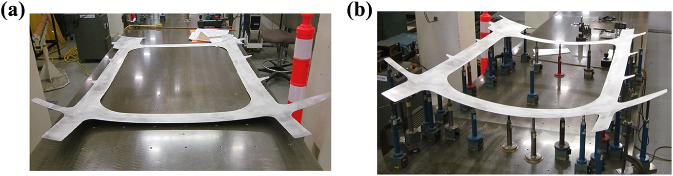
An aerospace panel: (a) in free state and (b) constrained on its inspection fixture set.⁷

For the time being, it is widely considered that a virtual inspection method, which is usually performed by numerical simulations to compensate for flexible deformation of nonrigid parts in free state, would significantly reduce the inspection time and cost.³ All inspection methods proposed so far are limited to linear elastic isotropic materials with well-known characteristics.^1

–7 Nowadays, the use of parts made of composite materials is progressively growing, especially in aerospace industry. However, up to now, there is no virtual inspection method that was developed for nonrigid composite parts, at least to the best of our knowledge. The reason is that the anisotropic nonlinear deformation behavior of nonrigid composite parts is much more complicated than that of linear isotropic elastic materials. Therefore, the deformation of composite parts could not be simulated correctly by finite element analysis without an appropriate material model for this purpose. A deep understanding of the behavior of nonrigid composite parts is not only very challenging but also very important for various applications such as developing specific virtual inspection methods for nonrigid composite parts.

It is remarked that the hyperelasticity gives an appropriate framework for numerical modeling of large deformation. In the last decades, the isotropic models have been developed to characterize the large deformation behavior of materials such as rubber-like materials (e.g. Mooney–Rivlin models⁸ and Ogden models⁹). There has been an increasing interest in the development of hyperelastic formulation for anisotropic materials because of its numerous industrial applications. A framework based on structural tensors for constitutive modeling of fiber-reinforced composites was established by Spencer.¹⁰ This approach was successfully used in modeling of fiber-reinforced composite behavior. Pham et al.¹¹ developed a transversely isotropic hyperelastic model to present the material behavior of glass-fiber–reinforced thermoplastic under large deformation of thermoforming process. In 2009, Aimène et al.¹² published an article in which they proposed a hyperelastic anisotropic material model and achieved good numerical simulation for the hemispherical punch forming. Peng et al.¹³ proposed an anisotropic hyperelastic constitutive model and demonstrated that it is suitable for modeling the large anisotropic deformation of a reinforced composite in double dome forming process. Recently, Gong et al.¹⁴ have successfully employed a hyperelastic constitutive model to simulate the behavior of glass/polypropylene prepregs during thermoforming process. The purpose of this article is to implement a hyperelastic shell to capture the large deformation behavior of a nonrigid composite part with application to the assembly process. It is also noted that several authors have implemented models of hyperelastic shell into finite element codes. Gruttmann and Taylor¹⁵ derived a rubber-like constitutive material model for membrane shells using principal stretches. Weiss et al.¹⁶ and Prot et al.¹⁷ developed a generalized approach for transversely isotropic membrane shells. Itskov¹⁸ derived an orthotropic hyperelastic material model for membrane shells with application to biological soft tissues and reinforced rubber-like structures. Tanaka et al.¹⁹ succeed to implement shell element for woven fabric composite materials with two families of fiber. These proposed methods were developed for fiber-reinforced composite materials or biological anisotropic materials that are generally characterized by low stiffness and large strains during the deformation. It was observed that the behavior of nonrigid composite parts in aerospace assembly process is quite different from the abovementioned material types. During assembly process, nonrigid part undergoes essentially large bending deformation due to geometric variations, gravity loads, and residual stress. In the literature, there exist very few studies investigating the behavior of nonrigid composite parts in assembly process. Therefore, the determination of a material model together with its parameters which is capable of capturing the large anisotropic deformation of nonrigid composite parts is the main purpose in this current research.

In this aticle, two strain–energy functions were studied for incompressible orthotropic hyperelastic material models able to capture the behavior of flexible fiber-reinforced thermoplastic composites (FRTPC). These models were implemented in the user-defined material (UMAT) subroutine of Abaqus for finite strain shell elements. The multilayered carbon-fiber–reinforced polyphenylene sulfide (CF/PPS) composite material, in which each layer is reinforced by two families of carbon fibers, was used in this study. In the modeling work, each layer was considered as an orthotropic material characterized by a strain–energy function. Material characterization works were carried out in order to identify the parameters of strain–energy functions. These material parameters were then used to simulate the deformation for the load test using a ball load applied on a large sheet of multilayer FRTPC. The deflections of the composite sheet predicted by numerical simulations performed with Abaqus were compared with the experimental data obtained from the load test in order to evaluate the capability of each material model used in this study.

Material model implementation

Generalized orthotropic hyperelastic material model for incompressible thin shells

In the present study, each point of the solid body B in the reference configuration Ω₀ is determined by the position vector X ∈ Ω₀ and in the current configuration Ω by the position vector x ∈ Ω (Figure 2). The deformation gradient F is defined by $F = \partial x / \partial X$ . For thin shell-like sheet, which has a plane stress state, the deformation gradient F has the following form:

F = (\begin{matrix} F_{11} & F_{12} & 0 \\ F_{21} & F_{22} & 0 \\ 0 & 0 & F_{33} \end{matrix})

Figure 2.

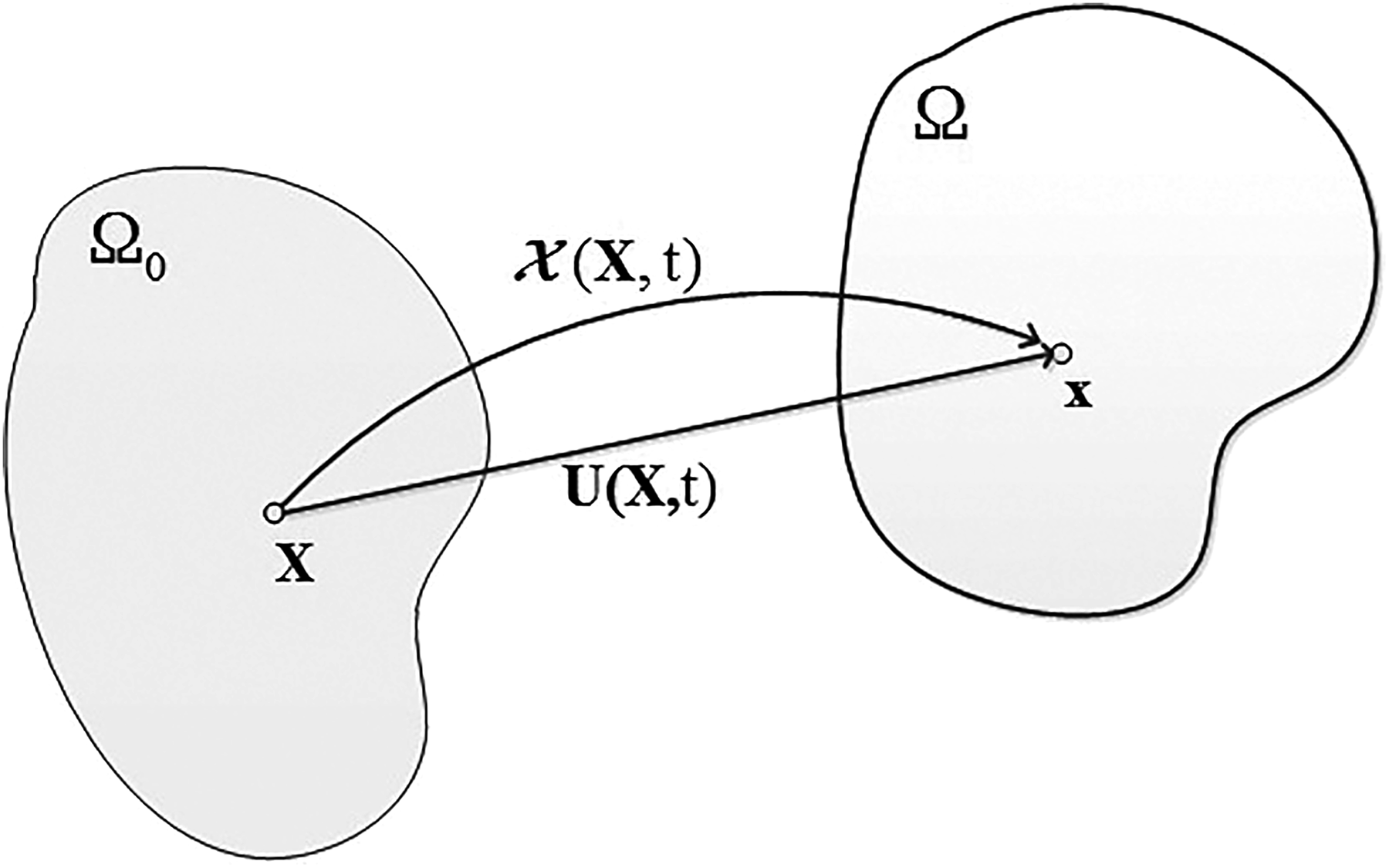
Motion of a continuum body.

For incompressible materials, $J = det F = 1$ . Hence, the following expression reads as

F_{33} = {(F_{11} F_{22} - F_{12} F_{21})}^{- 1}

The right Cauchy–Green deformation tensor is defined as $C = F^{T} F$ and the left Cauchy–Green deformation tensor is defined as $b = F F^{T}$ . The concept of hyperelasticity modeling is based on the existence of an energy potential, which is appropriate for the description of a large deformation including the anisotropic effect. In this study, the behavior of a thermoplastic reinforced by two families of fiber can be represented by the superposition of one isotropic model and two transversely isotropic models, which is given by

Ψ = Ψ_{iso} + Ψ_{trans}^{(1)} + Ψ_{trans}^{(2)}

Herein, Ψ_iso denotes the isotropic stored energy, and $Ψ_{trans}^{(1)} and Ψ_{trans}^{(2)}$ denote the transversely isotropic stored energy for the first and second fiber, respectively. The directions of the first and second fiber at point X are represented by unit vectors $a_{0} (X) and g_{0} (X)$ , respectively, in the reference configuration. For orthotropic materials, the initial directions of two fibers are orthogonal, that is, $a_{0} ⊥ g_{0}$ . During deformation, the vectors a₀ and g₀ are mapped onto the related current configuration such as $a = F a_{0} and g = F g_{0}$ . The vectors a₀, g₀, a, and g can be expressed on the basis of $(e_{1}, e_{2}, e_{3})$ as follows:

a_{0} = [\begin{matrix} cos θ_{1} \\ sin θ_{1} \\ 0 \end{matrix}], a = [\begin{matrix} F_{11} cos θ_{1} + F_{12} sin θ_{1} \\ F_{21} cos θ_{1} + F_{22} sin θ_{1} \\ 0 \end{matrix}]

g_{0} = [\begin{matrix} cos θ_{2} \\ sin θ_{2} \\ 0 \end{matrix}], g = [\begin{matrix} F_{11} cos θ_{2} + F_{12} sin θ_{2} \\ F_{21} cos θ_{2} + F_{22} sin θ_{2} \\ 0 \end{matrix}]

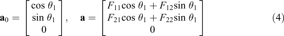
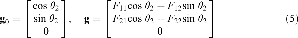
where θ₁ denotes the angle between e₁ and the fiber direction a₀; θ₂ denotes the angle between e₂ and the fiber direction g₀. For orthotropic materials, $θ_{2} = 90^{o} + θ_{1}$ . The strain–energy function Ψ in equation (3) for orthotropic materials can be expressed as a function of C and the fiber unit vectors a₀ and g₀ by

Ψ = Ψ_{iso} (C) + Ψ_{trans}^{(1)} (C, a_{0}) + Ψ_{trans}^{(2)} (C, g_{0})

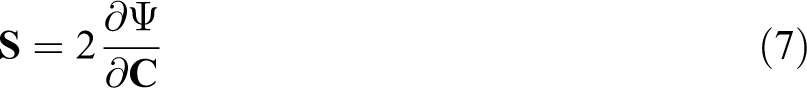
The mechanical behavior of the material is determined by the relationship between the second Piola–Kirchhoff stress tensor S and the right Cauchy–Green deformation tensor C as follows:

S = 2 \frac{\partial Ψ}{\partial C}

For incompressible orthotropic materials, the strain–energy function in equation (6) can be stated as a function of invariants of C,²⁰ which is given by

Ψ = Ψ (I_{1}, I_{2}, I_{4}, I_{6}) - \frac{1}{2} p (I_{3} - 1)

where the scalar p serves as an indeterminate Lagrange multiplier and five different invariants are defined by

I_{1} = tr (C), I_{2} = \frac{1}{2} [tr {(C)}^{2} - tr (C^{2})], I_{3} = det (C), I_{4} = a_{0} . C a_{0}, I_{6} = g_{0} . C g_{0}

where I₄ and I₆ represent the square of the stretching of fiber along their initial directions a₀ and g₀, respectively. Then, the second Piola–Kirchhoff stress tensor can be derived from equation (7), which is given by

S = 2 ω_{1} I + 2 ω_{2} (I_{1} I - C) + 2 ω_{4} a_{0} \otimes a_{0} + 2 ω_{6} g_{0} \otimes g_{0} + p C^{- 1}

where the symbol ⊗ denotes the tensor product, I is the second-order identity tensor, and

ω_{1} = \frac{\partial Ψ}{\partial I_{1}}, ω_{2} = \frac{\partial Ψ}{\partial I_{2}}, ω_{4} = \frac{\partial Ψ}{\partial I_{4}}, ω_{6} = \frac{\partial Ψ}{\partial I_{6}}

In the case of plane stress, the stress component S₃₃ vanishes. Therefore, the scalar p is obtained as follows:

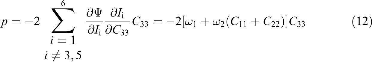
p = - 2 \sum_{\begin{matrix} i = 1 \\ i \neq 3, 5 \end{matrix}}^{6} \frac{\partial Ψ}{\partial I_{i}} \frac{\partial I_{i}}{\partial C_{33}} C_{33} = - 2 [ω_{1} + ω_{2} (C_{11} + C_{22})] C_{33}

where C₁₁, C₂₂, and C₃₃ are the components of right Cauchy–Green tensor C. On the other hand, the material elasticity tensor is determined by

\begin{matrix} C = 2 \frac{\partial S}{\partial C} = 4 (ω_{11} + 2 ω_{12} I_{1} + ω_{2} + I_{1}^{2} ω_{22}) I \otimes I - 4 (ω_{12} + I_{1} ω_{22}) (C \otimes I + I \otimes C) \\ + 4 ω_{22} C \otimes C - 4 ω_{2} I + 4 (ω_{14} + I_{1} ω_{24}) (a_{o} \otimes a_{o} \otimes I + I \otimes a_{o} \otimes a_{o}) \\ - 4 ω_{24} (a_{o} \otimes a_{o} \otimes C + C \otimes a_{o} \otimes a_{o}) + 4 ω_{44} a_{o} \otimes a_{o} \otimes a_{o} \otimes a_{o} \\ + 4 (ω_{16} + I_{1} ω_{26}) (g_{o} \otimes g_{o} \otimes I + I \otimes g_{o} \otimes g_{o}) \\ - 4 ω_{26} (g_{o} \otimes g_{o} \otimes C + C \otimes g_{o} \otimes g_{o}) \\ + 4 ω_{66} g_{o} \otimes g_{o} \otimes g_{o} \otimes g_{o} \\ + 2 C^{- 1} \otimes \frac{\partial p}{\partial C} + 2 p \frac{\partial C^{- 1}}{\partial C} \end{matrix}

where

\underset{\begin{array}{l} i = 1, 2, 4, 6 \\ j = 1, 2, 4, 6 \end{array}}{ω_{i j}} = \frac{\partial^{2} Ψ}{\partial I_{i} \partial I_{j}}

and I is the fourth-order identity tensor defined as

{(I)}_{ijkl} = \frac{1}{2} (δ_{ik} δ_{jl} + δ_{il} δ_{jk})

Strain–energy functions for CF/PPS materials

In this study, the mechanical response of CF/PPS material is represented by orthotropic incompressible hyperelastic models. PPS material is characterized as an isotropic matrix, in which carbon fibers are embedded. Carbon fibers are characterized by an exponential-type stress–strain behavior in the fiber direction. Two strain–energy functions were proposed and implemented for the incompressible CF/PPS material based on the polyconvexity conditions proposed by Balzani et al.²¹ The first proposed model is a modified function of a Holzapfel–Gasser–Ogden model.^22,23 The neo-Hookean model was used to determine the isotropic response of the matrix part. For the mechanical response of two families of carbon fibers, two exponential functions in terms of invariants were used. The strain–energy function of this model has the following form:

Ψ = M_{1} (I_{1} - 3) + k_{1} [e^{k_{2} {(I_{4} - 1)}^{2}} - 1] + k_{3} [e^{k_{4} {(I_{6} - 1)}^{2}} - 1] - \frac{1}{2} p (I_{3} - 1)

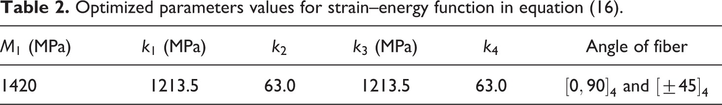
where M₁, k₁, k₂, k₃, and k₄ are the parameters of the strain–energy function in equation (16). The second proposed model uses the same energy function for the anisotropic part as in the first model, and the isotropic part is a function in terms of the invariants I₁ and I₂ ¹¹ as follows:

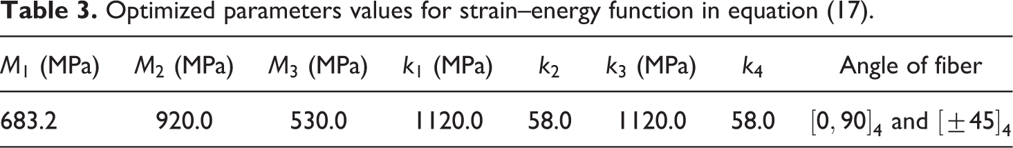
Ψ = M_{1} (I_{1} - 3) + M_{2} (I_{2} - 3) + M_{3} (I_{1} - 3) (I_{2} - 3) + k_{1} [e^{k_{2} {(I_{4} - 1)}^{2}} - 1] + k_{3} [e^{k_{4} {(I_{6} - 1)}^{2}} - 1] - \frac{1}{2} p (I_{3} - 1)

where M₁, M₂, M₃, k₁, k₂, k₃, and k₄ are the material parameters of the strain–energy function in equation (17).

Implementation in Abaqus/Standard UMAT

Several authors were successful to implement strain–energy functions into Abaqus through the UMAT subroutine.^17,19,24,25 In this article, the material models in equations (16) and (17) were implemented in Abaqus/Standard using the UMAT procedure. Abaqus requires only components of the Cauchy stress and the tangent stiffness matrix. The Cauchy stress tensor is determined by the push-forward operation of the stress tensor S to the current configuration²⁶ as shown in equation (18). It is noted that for thin shell element, the stress component in the thickness direction is neglected

σ = F S F^{T} = 2 ω_{1} b + 2 ω_{2} (I_{1} b - b^{2}) + 2 ω_{4} a \otimes a + 2 ω_{6} g \otimes g + p I

Based on Abaqus/Standard 6.13 documentation,²⁷ the Green–Naghdi stress rate is used for shell and membrane elements. The elasticity tensor C^∇ related to the Green–Naghdi stress rate is required for Abaqus user-defined subroutine and is computed as

{(C^{\nabla})}_{i j k l} = {(C^{o})}_{i j k l} - Λ_{i a k l} τ_{a j} + τ_{i a} Λ_{a j k l}

where Λ is a material-independent fourth-order tensor defined by Simo and Hughes,²⁸ and C^o is the elasticity tensor related to Zaremba–Jaumann objective rate defined as

{(C^{o})}_{i j k l} = {(\hat{C})}_{i j k l} + τ_{i k} δ_{j l} + τ_{j l} δ_{i k}

The spatial elasticity matrix $\hat{C}$ is defined by the push-forward operation of C in equation (13) as

{(\hat{C})}_{i j k l} = F_{i I} F_{j J} F_{k K} F_{l L} {(£)}_{I J K L}

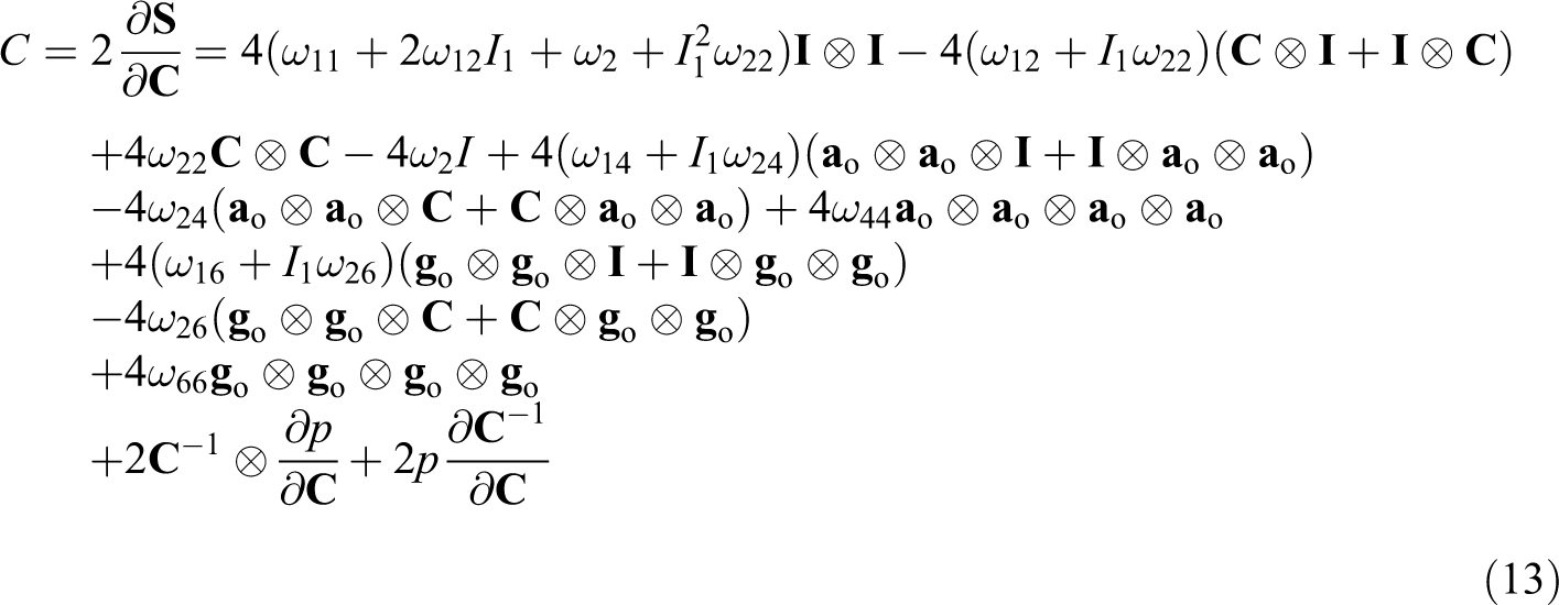
By replacing the formulation of C in equation (13) into equation (21), the spatial elasticity matrix $\hat{C}$ is obtained as

\begin{matrix} \hat{C} = 4 (ω_{11} + 2 ω_{12} I_{1} + ω_{2} + I_{1}^{2} ω_{22}) b \otimes b - 4 (ω_{12} + I_{1} ω_{22}) (b^{2} \otimes b + b \otimes b^{2}) \\ + 4 ω_{22} b^{2} \otimes b^{2} - 4 ω_{2} b ⊙ b + 2 I \otimes (F \frac{\partial p}{\partial C} F^{T}) - 2 p I \\ + 4 (ω_{14} + I_{1} ω_{24}) (a \otimes a \otimes b + b \otimes a \otimes a) - 4 ω_{24} (a \otimes a \otimes b^{2} + b^{2} \otimes a \otimes a) \\ + 4 ω_{44} a \otimes a \otimes a \otimes a + 4 (ω_{16} + I_{1} ω_{26}) (g \otimes g \otimes b + b \otimes g \otimes g) \\ - 4 ω_{26} (g \otimes g \otimes b^{2} + b^{2} \otimes g \otimes g) + 4 ω_{66} g \otimes g \otimes g \otimes g \end{matrix}

where the components of the fourth-order tensor b ⊙ b have the following form

{(b ⊙ b)}_{i j k l} = \frac{1}{2} (b_{i k} b_{j l} + b_{i l} b_{j k})

Material parameters identification

For materials whose stiffness is low and the large strain occurs during the deformation procedure, such as woven composites and biological tissues, the simple tensile test and/or biaxial test were usually used to characterize the material properties.^16,17 For assembly process, nonrigid composite parts undergo essentially the large bending deformation. Therefore, the three-point bending test that is considered more appropriate to characterize the bending properties of composite sheets was used in this study. The material parameters M₁, k₁, k₂, k₃, and k₄ of the strain–energy function in equation (16) and M₁, M₂, M₃, k₁, k₂, k₃, and k₄ of the strain–energy function in equation (17) for multilayered carbon-fiber–reinforced material were, respectively, determined by curve fitting by minimizing the discrepancy of loads between the experimental bending test data and numerical simulation using Abaqus.

Three-point bending test

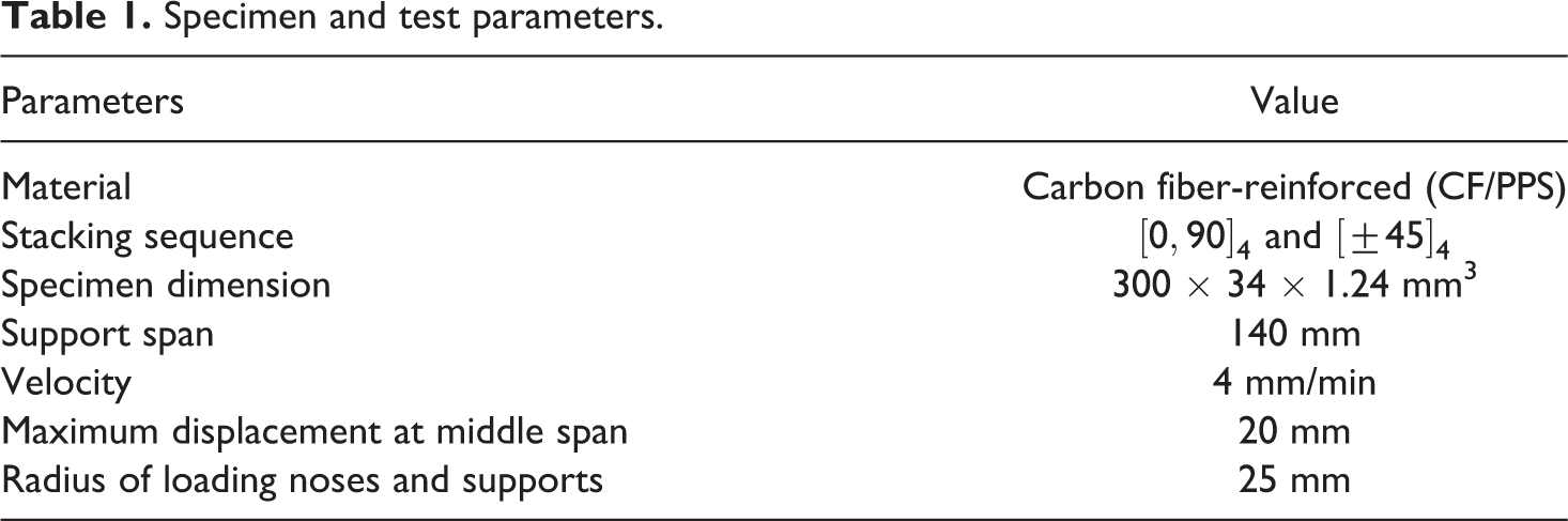
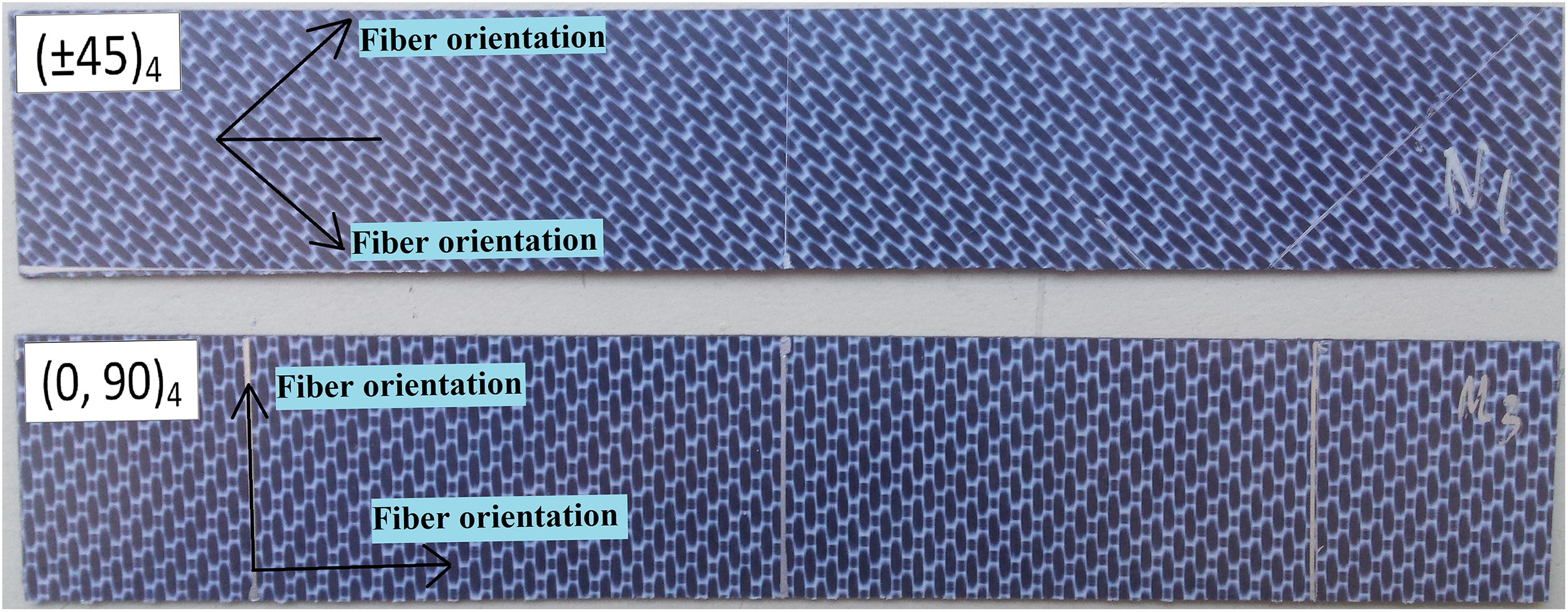
The composite material used in this study is a consolidated plate of four layers of CF/PPS. Each layer is composed of a PPS matrix and carbon fiber fabrics. The fiber volume fraction (V_f) is of 50%. The total thickness of the four-layer laminate is about 1.24 mm (0.31 mm per layer). Specimens with dimensions 300 × 34 × 1.24 mm³ were fabricated with two different stacking sequences ${[0, 90]}_{4} and {[\pm 45]}_{4}$ , as shown in Figure 3. Three-point bending tests were performed on the MTS testing machine with displacement control as shown in Figure 4. Five tests were conducted for each configuration as summarized in Table 1.

Figure 3.

Test specimens.

Figure 4.

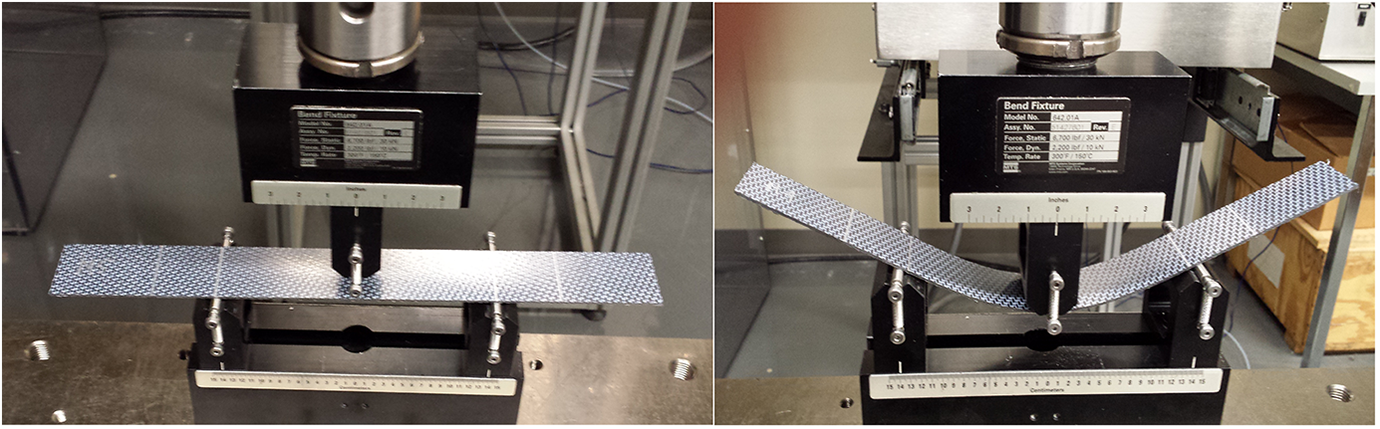
Three-point bending test using the MTS machine.

Table 1.

Specimen and test parameters.

Parameters	Value
Material	Carbon fiber-reinforced (CF/PPS)
Stacking sequence	${[0, 90]}_{4} and {[\pm 45]}_{4}$
Specimen dimension	300 × 34 × 1.24 mm³
Support span	140 mm
Velocity	4 mm/min
Maximum displacement at middle span	20 mm
Radius of loading noses and supports	25 mm

Computational experiment

Numerical simulation of the three-point bending test is created in Abaqus using UMAT subroutines developed for two strain–energy functions, that is, equations (16) and (17). Specimen is meshed with four-node shell elements (S4R in Abaqus/Standard) with a four-layer composite section. Each layer behaves like an orthotropic material. The computational model for the simulation of the three-point bending test with displacement control is depicted in Figure 5, where frictionless contact between supports and specimen was defined.

Figure 5.

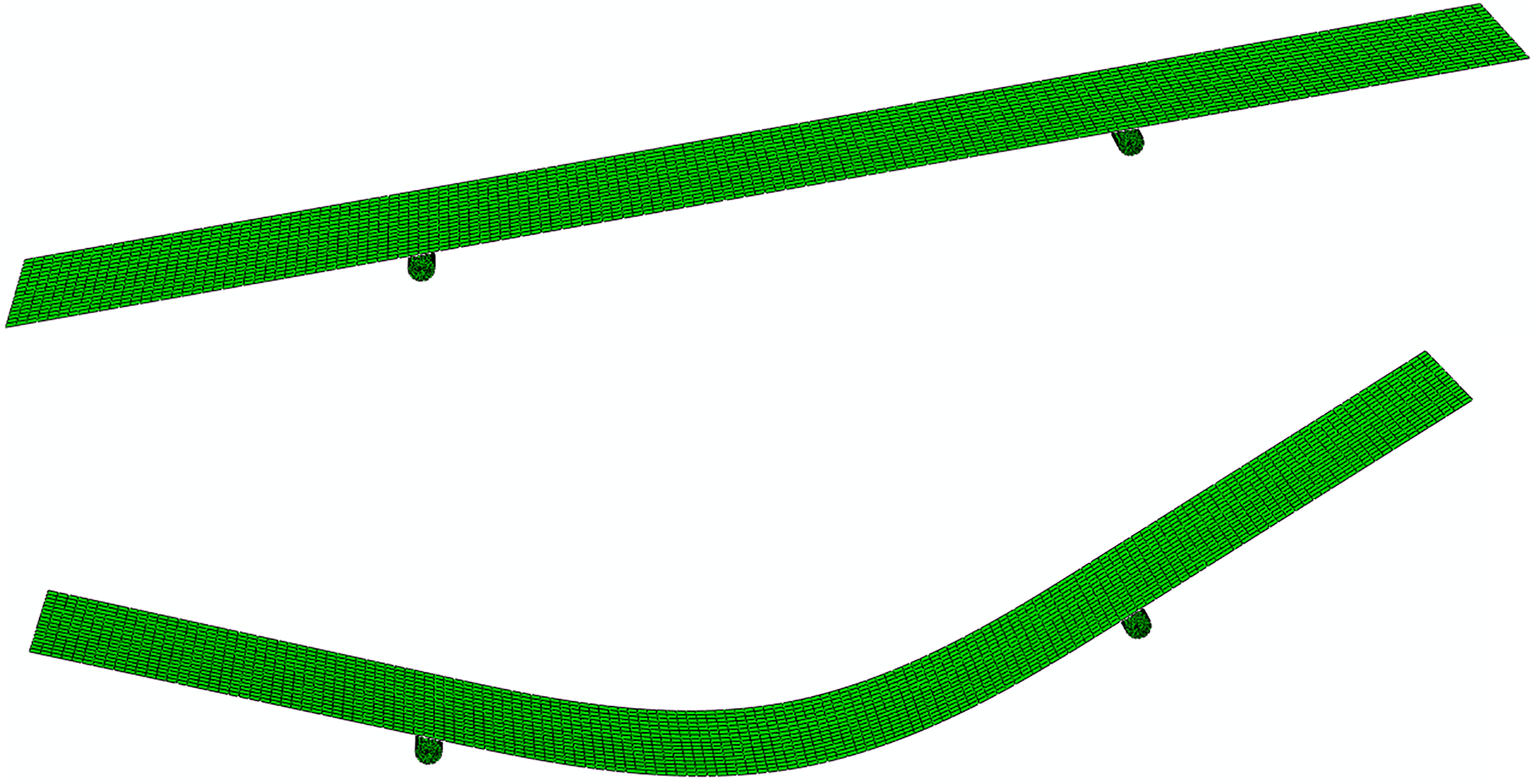
Finite element modeling for three-point bending test.

Inverse characterization method

The inverse characterization method allows identifying the material parameters of the strain–energy functions by minimizing the difference of loads between the experimental test data and numerical simulation. For this fitting process, the following objective function was used together with the adaptive response surface optimization method:

Y = min [\sum_{i = 1}^{N} {(F_{i}^{exp} - F_{i}^{s i m u})}^{2}]

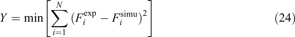
Herein, N denotes the number of steps at which loads were measured, and $F_{i}^{exp} and F_{i}^{s i m u}$ denote the experimental load and the computed load, respectively, at step i. A good agreement was found between the predicted results and experimental data for both strain–energy functions in equations (16) and (17) as well as for both stacking sequences ${[0, 90]}_{4} and {[\pm 45]}_{4}$ , as depicted in Figure 6. The material parameters obtained from the curve fitting for strain–energy functions in equations (16) and (17) are presented in Tables 2 and 3, respectively. In order to evaluate the accuracy of the curve fitting, the relative error, denoted by $\bar{r}$ , is calculated as follows:

\bar{r} = \frac{1}{| F_{max}^{exp} |} \sqrt{\frac{1}{N} \sum_{i = 1}^{N} {(F_{i}^{exp} - F_{i}^{simu})}^{2}}

Figure 6.

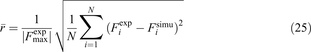
Comparison between numerical results and experimental data: (a) strain–energy function in equation (16); (b) strain–energy function in equation (17).

Table 2.

Optimized parameters values for strain–energy function in equation (16).

M₁ (MPa)	k₁ (MPa)	k ₂	k₃ (MPa)	k ₄	Angle of fiber
1420	1213.5	63.0	1213.5	63.0	${[0, 90]}_{4} and {[\pm 45]}_{4}$

Table 3.

Optimized parameters values for strain–energy function in equation (17).

M₁ (MPa)	M₂ (MPa)	M₃ (MPa)	k₁ (MPa)	k ₂	k₃ (MPa)	k ₄	Angle of fiber
683.2	920.0	530.0	1120.0	58.0	1120.0	58.0	${[0, 90]}_{4} and {[\pm 45]}_{4}$

where $F_{max}^{exp}$ denotes the experimental load at the last step.

Results showed that the relative errors of the curve fitting are small, with $\bar{r}$ = 0.0182 and $\bar{r}$ = 0.0160, respectively, for the strain–energy functions in equations (16) and (17). It turned out that the mechanical response of the composite reinforced by two families of carbon fiber was well modeled by the exponential function $Ψ_{t r a n s}^{(HGO) (α)}$ , and, globally, the strain–energy function in equation (17) is more appropriate for the mechanical behavior of multilayered CF/PPS in the three-point bending test.

Model validation and discussion

To validate the material models used in this study, a load test with a large sheet of multilayered FRTPC was performed. This test is chosen because the deformation in this load test is quite similar to that in assembly process. The bending displacement of the composite sheet predicted by numerical simulations using Abaqus was compared with the experimental results from the load test.

Experimental test

Table 4 summarizes experimental parameters used in this work. The material used here is the same as the material used in the three-point bending test presented above. The thickness of the four-layer laminate is 1.24 mm (0.31 mm per layer) with the stacking sequence ${[0, 90]}_{4}$ . A plate with dimensions 930 × 890 ×1.24 mm³ was used. This plate lies on four rigid sphere-head supports and undergoes bending deformation imposed by a 3.63-kg ball applied at center point (see Figure 7). The vertical displacement of the plate was measured using a 3D Measuring Arm developed by Keron at 110 points on the plate surface. Three measurements were performed to get average values. The deviation values of the measurement at these points are depicted in Figure 8. The maximum deviation value is about 1.24 mm, which corresponds to a maximum relative error of 5.42%.

Table 4.

Experimental parameters.

Composite plate
Material	CF/PPS
Stacking sequence	${[0, 90]}_{4}$
Plate dimension	930 × 890 × 1.24 mm³
Supports system
Radius of sphere-head supports	6.35 mm
Height of four supports	30.5 ± 0.32 mm
Distance between supports (Figure 7)	660.4 ± 0.95 mm
Steel ball
Radius of steel ball	49.5 mm
Weight of steel ball	3.63 kg
Deviation of ball position from the center point (Figure 7)	±2.15 mm

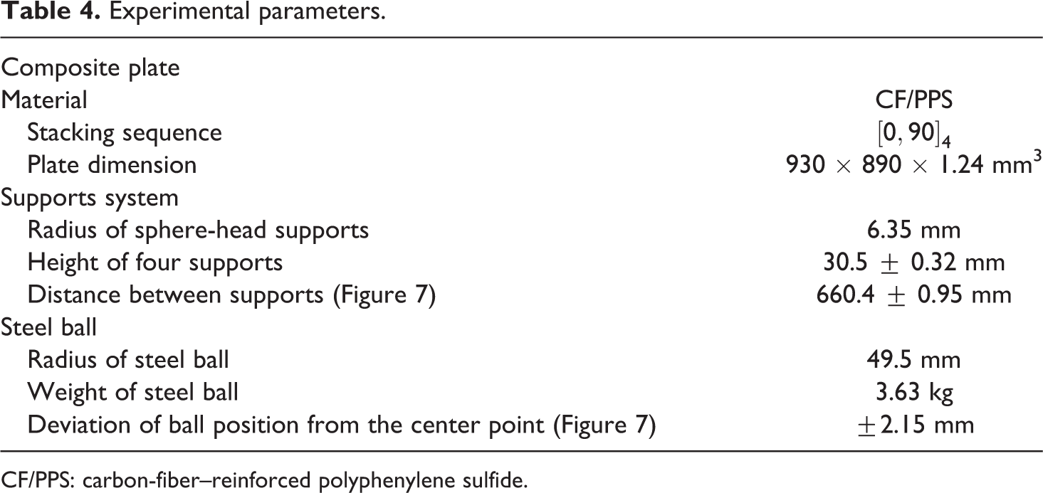
CF/PPS: carbon-fiber–reinforced polyphenylene sulfide.

Figure 7.

Bending load test set-up.

Figure 8.

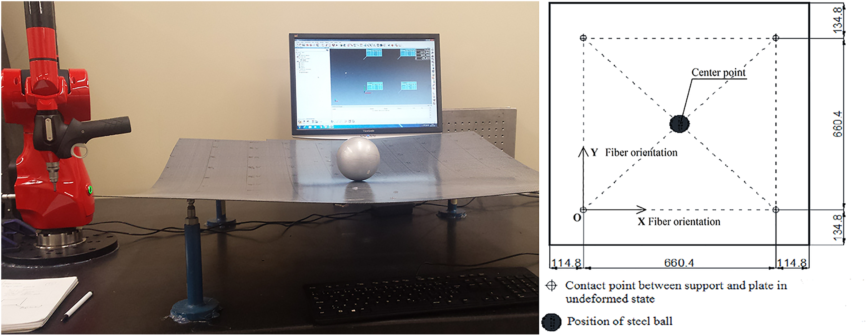
Measurement deviation of vertical displacement (mm).

Test simulation and result discussion

A finite element computational procedure that corresponds to the plate bending test introduced in the previous section is developed with Abaqus using a UMAT with parameters presented in Tables 2 and 3. The element type used in Abaqus is shell element (S4R) with a four-layer composite section. The specimen lies on four rigid spheres which represent supports used in the experiment. Frictionless contact between the specimen and supports is defined. A 35.59-N load, which is equivalent to the weight of the steel ball, is applied on the plate at the same location as in the experimental test (at the center point). The experimental data and simulated results were compared in terms of bending displacement along the 10 paths, as shown in Figure 9. The comparison of experimental and simulated vertical displacement along these paths is presented in Figure 10. The maximum and minimum differences between experimental and numerical results are summarized in Table 5.

Figure 9.

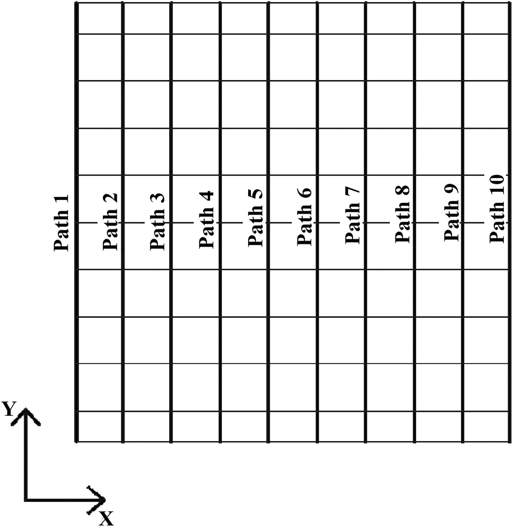
Path positions along Y-axis.

Figure 10.

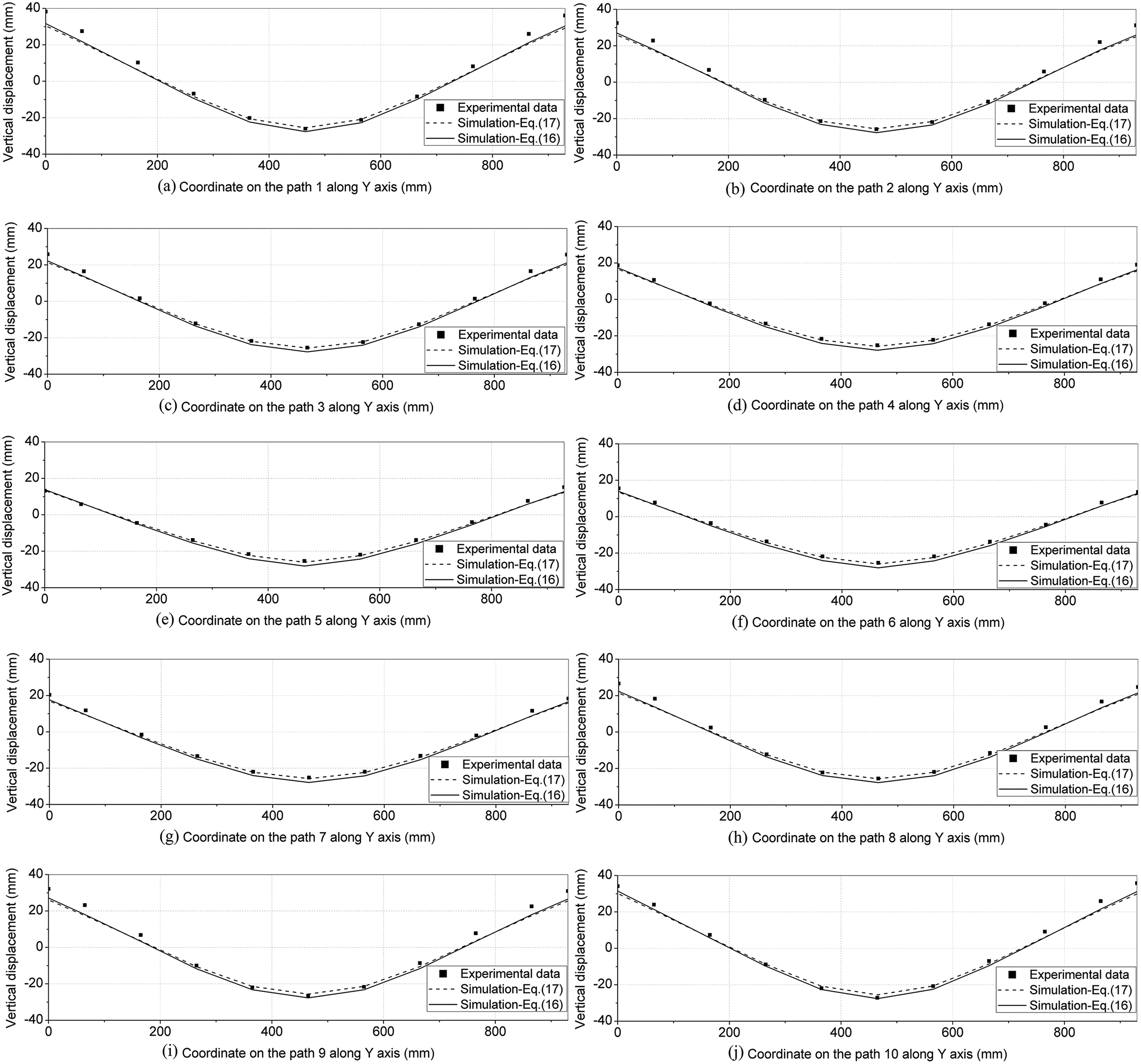
Result comparison ((a) path 1, (b) path 2, (c) path 3, (d) path 4, (e) path 5, (f) path 6, (g) path 7, (h) path 8, (i) path 9, and (j) path 10).

Table 5.

Maximum and minimum difference in vertical displacement between experimental and simulation data on each path.

Path	Strain–energy function in equation (16)		Strain–energy function in equation (17)
Path	Minimum (mm)	Maximum (mm)	Minimum (mm)	Maximum (mm)
Path 1	1.53	6.56	0.31	7.87
Path 2	1.34	5.44	0.04	6.56
Path 3	1.43	4.56	0.17	5.36
Path 4	1.14	2.81	0.24	3.39
Path 5	0.47	2.78	0.16	2.92
Path 6	0.79	2.73	0.38	2.15
Path 7	1.66	2.84	0.26	3.55
Path 8	1.43	4.57	0.15	5.17
Path 9	1.191	5.22	0.27	6.10
Path 10	0.50	4.62	0.08	5.86

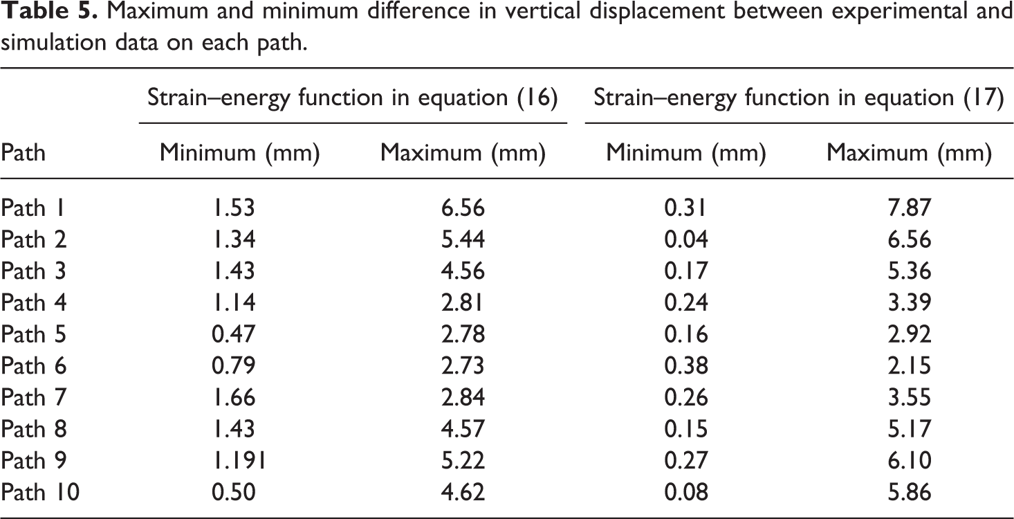
Figure 10 shows that at the middle of the plate (paths 4–8), the simulation gives better agreement with the experimental data than on the contour of the plate (paths 1–3 and paths 8–10). The maximum difference between simulation and experiment, 6.56 mm for strain–energy functions in equation (16) and 7.87 mm for strain–energy function in equation (17), appears at the boundary of the plate (path 1; see Table 5).

The average discrepancies between the experimental and the numerical results are 3.64 and 3.39 mm, respectively, for the strain–energy functions in equations (16) and (17), which are quite small in comparison with the dimensions of the composite sheet. It demonstrates that the simulations with two orthotropic hyperelastic models used in this study gave good agreements with the experimental results. It is remarked that the strain–energy function of equation (17) provided better response than that of equation (16).

Conclusion

This article presents the implementation of two orthotropic hyperelastic models used for assessing the mechanical behavior of multilayer FRTPC sheets. These models were developed based on the polyconvexity condition of strain–energy function and implemented in the UMAT subroutine of Abaqus for finite strain shell elements. The material parameters were numerically identified by fitting numerical simulation results to experimental results obtained from three bending tests for both stacking sequences ${[0, 90]}_{4} and {[\pm 45]}_{4}$ . These models were then validated through the ball load test on a large composite sheet. Results showed that

Both proposed orthotropic hyperelastic models are appropriate for the CF/PPS multilayer composite material.

The parameters of these models can be well identified in three-point bending tests with two different fiber orientation configurations.

The numerical simulation using shell element (S4R) with the composite section of four layers in Abaqus is good enough for the multilayer FRTPC sheets.

These material models responded well the validation case of the ball load test on a large CF/PPS multilayer composite sheet.

Footnotes

Acknowledgments

The authors would like to thank the National Sciences and Engineering Research Council and our industrial partners for their support and financial contribution.

Declaration of Conflicting Interests

The author(s) declared no potential conflicts of interest with respect to the research, authorship, and/or publication of this article.

Funding

The author(s) received no financial support for the research, authorship, and/or publication of this article.

ORCID iD

Ngoc-Hung Vu

Vincent François

References

Abenhaim

Tahan

Desrochers

. A novel approach for the inspection of flexible parts without the use of special fixtures. J Manuf Sci Eng 2011; 133(1): 011009-1-011009-11.

Abenhaim

Desrochers

Tahan

. Nonrigid parts’ specification and inspection methods: notions, challenges, and recent advancements. Int J Adv Manuf Technol 2012; 63: 741–752.

Aidibe

Tahan

Abenhaim

. Distinguishing profile deviations from a part’s deformation using the maximum normed residual test. WSEAS Trans Appl Theor Mech 2012; 7: 11.

Aidibe

Tahan

. Adapting the coherent point drift algorithm to the fixtureless dimensional inspection of compliant parts. Int J Adv Manuf Technol 2015; 79: 831–841.

Abenhaim

Desrochers

Tahan

. A virtual fixture using a FE-based transformation model embedded into a constrained optimization for the dimensional inspection of nonrigid parts. Comput-Aided Des 2015; 62: 248–258.

Sabri

Tahan

Pham

. Fixtureless profile inspection of non-rigid parts using the numerical inspection fixture with improved definition of displacement boundary conditions. Int J Adv Manuf Technol 2016; 82: 1343–1352.

Sattarpanah Karganroudi

Cuillière

J-C

Francois

. Automatic fixtureless inspection of non-rigid parts based on filtering registration points. Int J Adv Manuf Technol 2016; 87: 687–712.

Rivlin

. Large elastic deformations of isotropic materials. In: GI

Barenblatt

Joseph

(eds) Collected papers of RS Rivlin: Volume I and II. New York: Springer, 1997, pp. 90–108.

Ogden

. Non-linear elastic deformations. Paris, France: John Wiley, 1984.

10.

Spencer AJM and International Centre for Mechanical S. Continuum theory of the mechanics of fibre-reinforced composites. Wien, Austria: Springer-Verlag, 1984.

11.

Pham

X-T

Bates

Chesney

. Modeling of thermoforming of low-density glass mat thermoplastic. J Reinf Plast Compos 2005; 24: 287–298.

12.

Aimène

Vidal-Sallé

Hagège

. A hyperelastic approach for composite reinforcement large deformation analysis. J Compos Mater 2009; 44: 5–26.

13.

Peng

Guo

. A simple anisotropic hyperelastic constitutive model for textile fabrics with application to forming simulation. Compos B Eng 2013; 52: 275–281.

14.

Gong

Peng

Yao

. An anisotropic hyperelastic constitutive model for thermoplastic woven composite prepregs. Compos Sci Technol 2016; 128: 17–24.

15.

Gruttmann

Taylor

. Theory and finite element formulation of rubberlike membrane shells using principal stretches. Int J Numer Methods Eng 1992; 35: 1111–1126.

16.

Weiss

Maker

Govindjee

. Finite element implementation of incompressible, transversely isotropic hyperelasticity. Comput Methods Appl Mech Eng 1996; 135: 107–128.

17.

Prot

Skallerud

Holzapfel

. Transversely isotropic membrane shells with application to mitral valve mechanics. Constitutive modelling and finite element implementation. Int J Numer Methods Eng 2007; 71: 987–1008.

18.

Itskov

. A generalized orthotropic hyperelastic material model with application to incompressible shells. Int J Numer Methods Eng 2001; 50: 1777–1799.

19.

Tanaka

Noguchi

Fujikawa

. Development of large strain shell elements for woven fabrics with application to clothing pressure distribution problem. Comput Model Eng Sci 2010; 62(3): 265–290.

20.

Spencer

AJM

. Theory of fabric-reinforced viscous fluids. Composites Part A 2000; 31: 1311–1321.

21.

Balzani

Neff

Schröder

. A polyconvex framework for soft biological tissues. Adjustment to experimental data. Int J Solids Struct 2006; 43: 6052–6070.

22.

Holzapfel

Gasser

Ogden

. A new constitutive framework for arterial wall mechanics and a comparative study of material models. J Elast 2000; 61: 1–48.

23.

Nolan

Gower

Destrade

. A robust anisotropic hyperelastic formulation for the modelling of soft tissue. J Mech Behav Biomed Mater 2014; 39: 48–60.

24.

Peng

Guo

Zia-Ur-Rehman . A simple anisotropic fiber reinforced hyperelastic constitutive model for woven composite fabrics. Int J Mater Form 2010; 3: 723–726.

25.

Suchocki

. A finite element implementation of Knowles stored-energy function: theory, coding and applications. Arch Mech Eng 2011; 58: 319.

26.

Holzapfel

. Nonlinear solid mechanics: a continuum approach for engineering. Chichester, UK: Wiley, 2000.

27.

Abaqus. Using Abaqus Online Documentation, Version 6.13, Dassault Systèmes Simulia Corp., Providence, RI, USA. http://129.97.46.200:2080/v6.13 (2013, accessed 26 September 2016).

28.

Simo

Hughes

TJR

. Computational inelasticity. New York, NY: Springer, 1998, p. XIV, 392.

Characterization of multilayered carbon-fiber–reinforced thermoplastic composites for assembly process

Abstract

Keywords

Introduction

Material model implementation

Generalized orthotropic hyperelastic material model for incompressible thin shells

Strain–energy functions for CF/PPS materials

Implementation in Abaqus/Standard UMAT

Material parameters identification

Three-point bending test

Computational experiment

Inverse characterization method

Model validation and discussion

Experimental test

Test simulation and result discussion

Conclusion

Footnotes

Acknowledgments

Declaration of Conflicting Interests

Funding

ORCID iD

References