Sage Journals: Discover world-class research

Abstract

In the lay-up process of thermoplastic composite tape, the thermal conditions have great influence on the end quality and performance of composites. In the lay-up process of thermoplastic matrix composites, a semi-infinite solid model is used to analyse the heat transfer by simulating the heating of hot gas torch. Temperature of the control volume is calculated based on the model. A dynamic finite element model is developed to obtain the transient temperature field. The birth–death element strategy in ANSYS was used to simulate the movement of lay-up head during dynamic loading and laying-up prepreg onto the composite substrate. The simulation results of using the transient heat transfer model and the finite element model were compared well. The bonding temperature increases linearly with the heater temperature and is closely related to the moving speed of the roller. The bonding temperature changed slowly when the roller moved faster.

Keywords

Finite element analysis lay-up temperature field thermoplastic composite heat transfer

Introduction

In recent years, thermoplastic composites are commonly used in the composite manufacturing processes such as filament winding and tape lay-up. Many studies have been devoted to develop this promising composite manufacturing technique.^1

–9 Pitchumani et al. built theoretical models for the physical phenomena governing interfacial bonding and void dynamics (growth and consolidation) during processing. The effects of several processing conditions and the placement head configurations on the bonding level and final void content were illustrated.² Thermal history during the manufacturing processes has a significant influence on the final quality of composite component. Therefore, the temperature field during thermoplastic composites tape lay-up process was studied.^{10

–21} Wagner and Colton¹² established a mathematical model for temperature field in the composite filament winding process and simulated the process using ABAQUS (ABAQUS Inc., USA). Tumkor et al.¹⁴ developed the mathematical model of the temperature field using the finite difference method, providing the numerical solution of the temperature field that varies with time. Guan and Pitchumani¹⁵ studied the heat conduction problems during the thermoplastic composite placement process when hot gas was emitted from heat source. The Nusselt number near the nip point was mainly studied based on the Crystal Dynamics. Hassan et al.¹⁶ established a three-dimensional heat conduction model during autoclave forming process of thermoset composites. The eight-node matrix unit was used based on the Lagrange equation, and a computer code solving the model was given. Trende et al.²¹ modelled the process of double-belt press lamination of thermoplastic composite laminates. Temperature-dependent thermal properties and non-infinite contact conductance at material interfaces were included. Zhao et al.²² proposed a simulation model based on ANSYS (ABAQUS Inc., USA) to predict the thermal history and induced thermal stresses in thermoplastic composite rings.

The compaction roller moves continuously and the tape is continuously laid-up onto the surface of the composite substrate ply by ply. Here, a heat transfer model is developed and the dynamic finite element is used to simulate the transient temperature field of the composite–mandrel assembly of the lay-up process. By comparison, the transient heat transfer model is proved to be correct. The finite element model has been developed with the following features: (a) birth–death element strategy in ANSYS was used to simulate the addition of prepreg onto the composite substrate and (b) to simulate the movement of lay-up head using a dynamic loading strategy.

Transient temperature field analysis in the thermoplastic composite tape lay-up process

Heat transfer in the lay-up process

Thermoplastic composite tape lay-up process, also known as automated fibre placement (AFP), is shown in Figure 1. The compaction roller moved at a constant speed to consolidate the continuous tape (prepreg) onto the surface of the substrate, while providing the heat through hot gas. The nip point is the location where the incoming prepreg comes into contact with the substrate. The temperature of nip point had a great influence on the performance of composite components, although the volume of nip point was small. A transient heat transfer model was developed to obtain the temperature field near the nip point.

Figure1.

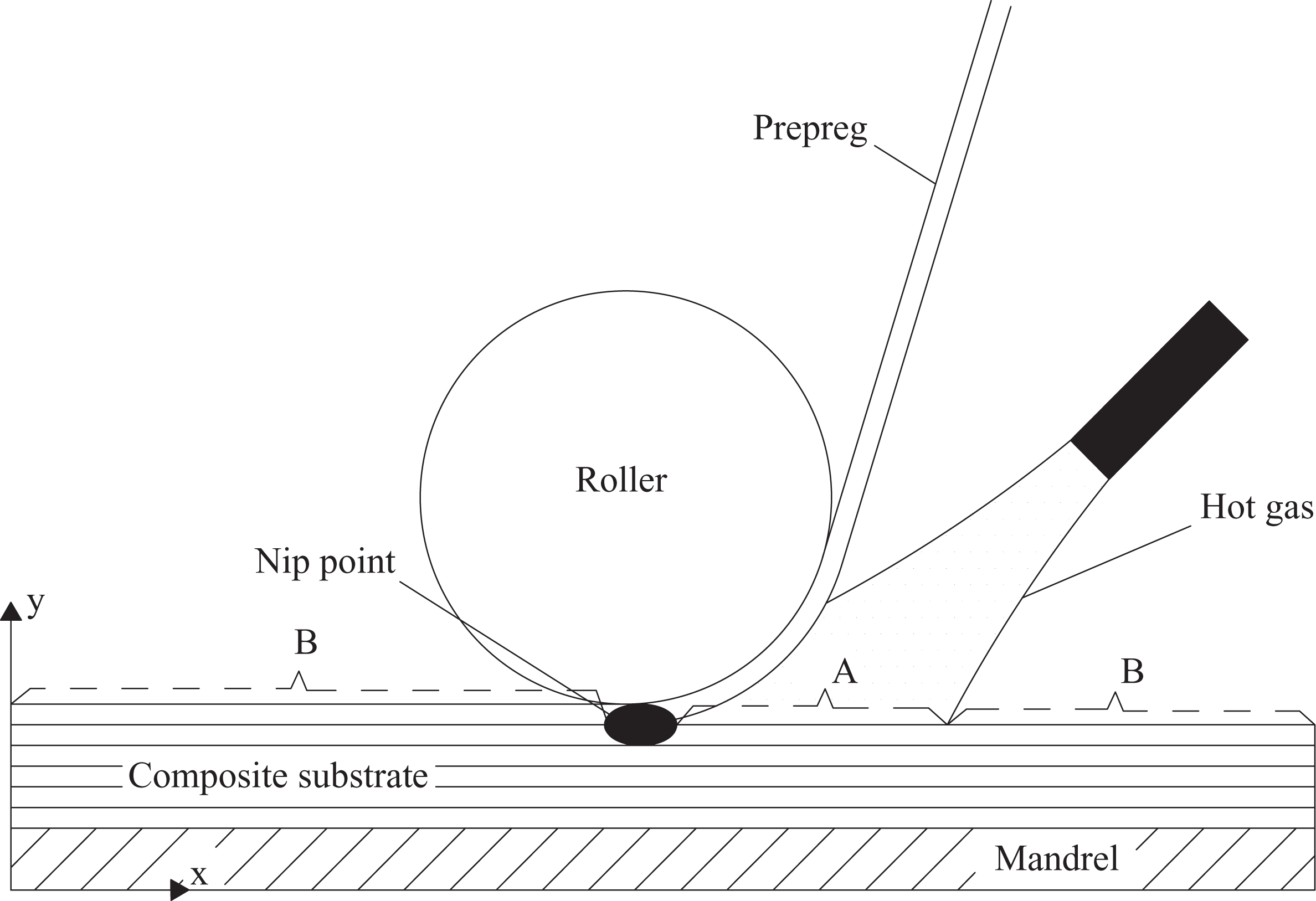
Schematic diagram of the thermoplastic composite prepreg lay-up process. A: boundary impacted by high temperature gas. B: boundary under the natural convection.

To simplify the analysis, a semi-infinite solid model was used to simulate heat transfer in the AFP process. This model can be described as a body having a single plane surface and extends to infinity in all directions. The composite–mandrel assembly in the lay-up process could be modelled as a semi-infinite medium, since the variation in temperature in the region near the surface of the substrate (nip point) is of our interest. For both the composite and the mandrel, the heat transfer followed the one-dimensional heat conduction differential equation

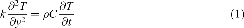
k \frac{\partial^{2} T}{\partial y^{2}} = ρ C \frac{\partial T}{\partial t}

where k is the thermal conductivity, ρ is the density, C is the specific heat. On the surface of the composite substrate, heat transfer follows the Newton cooling equation

q = h (T_{w} - T_{f})

where q is the heat flux, T _w and T _f are temperature on the solid surface and fluid temperature, respectively. After applying a constant heat source T _∞, the temperature field at any time can be obtained²³ by the equation

\frac{T (y, t) - T_{i}}{T_{\infty} - T_{i}} = e r f c (\frac{y}{2 \sqrt{α t}}) - exp (\frac{h y}{k} + \frac{h^{2} α t}{k^{2}}) e r f c (\frac{y}{2 \sqrt{α t}} + \frac{h \sqrt{α t}}{k})

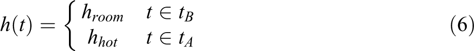
where T_i and T _∞ are the temperature on the solid surface and gas temperature, respectively. α is the thermal diffusivity, k is the thermal conductivity and h is the convection heat transfer coefficient. As the heater position changes during the lay-up process, the hot gas temperature T _∞ cannot be considered as a constant. The gas temperature near any point of composite substrate surface can be gained by the equation

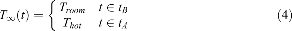
T_{\infty} (t) = \{\begin{matrix} T_{r o o m} & t \in t_{B} \\ T_{h o t} & t \in t_{A} \end{matrix}

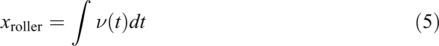
where t _A represents the time interval, while the composite substrate is exposed to hot air from 500°C to 800°C and t _B represents the time interval, while the substrate is exposed to air at a temperature of 25°C. Displacement of the roller can be expressed by integrating the moving speed ν,

x_{r o l l e r} = \int ν (t) d t

The convective heat transfer coefficients at any moment during the AFP process can be expressed as follows

h (t) = {\begin{matrix} h_{r o o m} & t \in t_{B} \\ h_{h o t} & t \in t_{A} \end{matrix}

Composite surface is divided into regions A and B according to different convective heat conditions. In region A, the substrate is heated by hot gas. In region B, the composite substrate is cooled by room air.

Transient temperature field analysis

The Imperial Chemical Industries’ (Amsterdam, The Netherlands) aromatic polymer composite (APC-2) is used in the study, whose density is 1562 kg/m³. Thermal conductivity and specific heat at different temperatures are shown in Table 1.¹⁴

Table 1.

The thermal conductivity and specific heat capacity of APC-2.

T (°C)	k(x) (W/mK)	k(y) (W/mK)	C (W/mK)
0	0.6	6	800
60	0.65	6.5	908
120	0.7	7	1016
180	0.75	7.5	1124
240	0.8	8	1232
300	0.85	8.5	1340
360	0.9	9	2080
390	0.95	9.25	1660
420	0.9	9.5	1663
480	0.9	10	1664

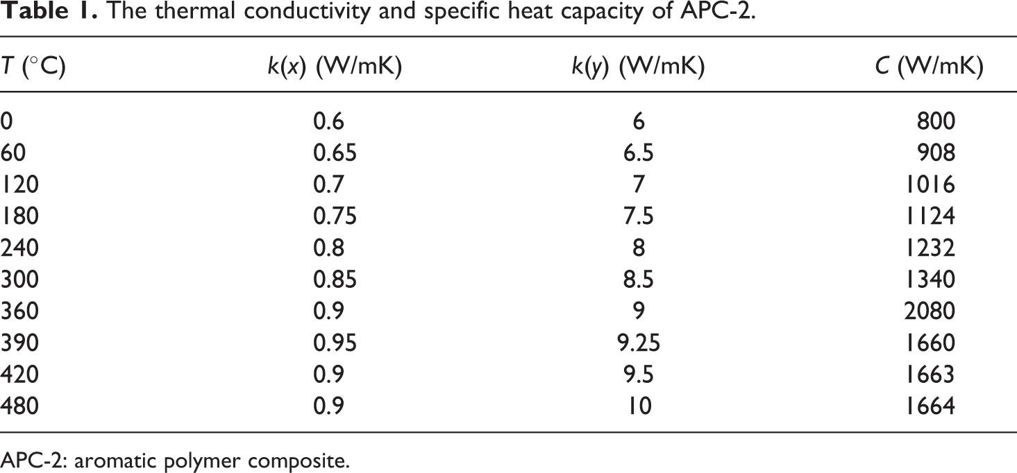
APC-2: aromatic polymer composite.

When composite is heated by hot gas, convective heat transfer coefficient varies widely. Convective heat transfer coefficient can be calculated²³ as follows

h = \frac{k}{L_{c}} N u

where Nu is the Nusselt number. In region A, where the substrate is heated by hot gas, Nu can be calculated by

N u = 0 {.228 R e}^{0.731} {Pr}^{\frac{1}{3}}

where $Re$ is the Reynolds number:

Re = \frac{υ L_{c}}{ν}

where υ is the speed of hot gas coming out of the heater nozzle, physical properties k, Pr and ν are decided by film temperature $T_{f} = \frac{T_{S} - T_{\infty}}{2}$ . At high temperature and high speed, physical properties of hot gas changes significantly. Then T _∞ should be replaced by the reference temperature T*²³

T_{*} = T_{\infty} + 0.5 (T_{w} - T_{\infty}) + 0.22 (T_{r} - T_{\infty})

When the film temperature is within the range from 400°C to 850°C, convective heat transfer coefficients are calculated by substituting equation (8) into equation (7) (as shown in Table 2). The speeds of hot gas coming out of the heater nozzle are 650m/s and 800m/s, respectively.

Table2.

The surface heat transfer coefficient of APC-2 at the impact of high-speed hot air.

T (°C)	υ = 650 mm/s	υ = 800 mm/s
400	953.4	1109.8
450	950.5	1106.4
500	947.2	1102.5
550	942.5	1097.1
600	940.8	1094.2
650	936.0	1089.5
700	933.2	1086.2
750	928.1	1080.2
800	925.4	1076.7
850	922.3	1073.2

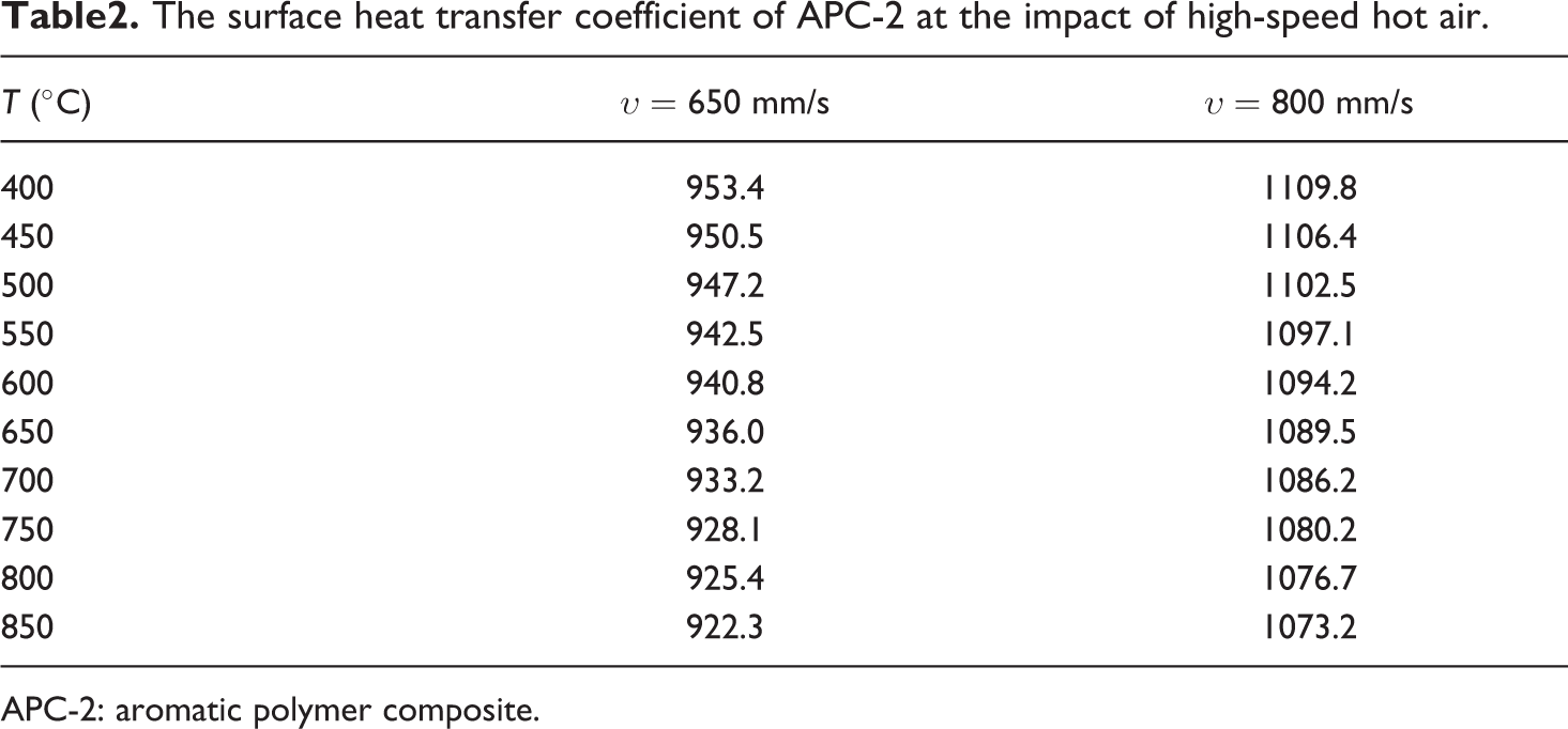
APC-2: aromatic polymer composite.

It can be found from the data of Table 2 that higher surface heat transfer coefficient can be obtained by high hot gas speed, and in the range from 400°C to 850°C, the surface heat transfer coefficient is reduced slightly as the temperature increases.

The boundary conditions are considered as follows

T_{\infty} = 600^{\circ} C

υ = 650 m / s

δ = 0.125 m m

L = 60 m m

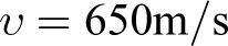
where T _∞ is the temperature of hot gas, υ is the speed of hot gas, δ is the thickness of each layer and L is the length of mandrel. Temperature of the control volume (as shown in Figure 2(a)) in the first lay-up process is calculated using MATLAB (MathWorks Inc., USA). As the lay-up head moves from the left edge of mandrel to the control volume, temperature maintains 25°C (c 1), because the control volume is not heated by hot gas. When the lay-up head moves over the control volume, the temperature reaches a peak value (c 2) rapidly. As the lay-up head moves to the right edge of mandrel, the control volume is cooled (c 3).

Figure 2.

(a) Solving process for temperature of control volume in the first lay-up process. (b) Temperature of control volume in the whole (six) lay-up process.

Substituting both initial conditions and boundary conditions into equation (3), temperature of the control volume is solved in the whole (six) lay-up process (as shown in Figure 2(b)). In Figure 2(b), curves I to IV indicates temperature in six lay-up processes, respectively. Some features can be found as follows:

Each curve has a peak value of temperature, which represent the temperature of control volume when lay-up head moves over.

The first peak temperature is much lower, resulting from the strong heat absorption of mandrel.

The second peak temperature is the highest due to two main reasons. One is the temperature has risen to a higher level due to the accumulation of heat; another is the control volume (in first layer) is heated directly by hot gas, when the second layer is laid up.

Dynamic finite element simulation based on ANSYS

Finite element modelling and assumptions

To use carbon fibre-reinforced thermoplastic matrix composite APC-2, the AFP process is simulated with the finite element method. In the actual process of AFP, the corner region formed by the prepreg and the substrate is subjected to the welding of hot gas, where the prepreg and the substrate are bonded and the nip point is then formed. Obviously under the action of the heat source from the outermost layer, the state with different temperature gradients is formed below each layer and between each layer, and the distribution of temperature field changed considerably with time, which can be viewed as transient heat transfer process; therefore, the thermal module is used to analyse transient heat transfer in the composite substrate. To simply this model, the following assumptions are made.^3
,5

Each ply is considered to be a plate.

The effect of heat dissipation of compaction roller along the width can be neglected, as the plate is large enough, the width of roller can be neglected.

The composite substrate is evenly heated by the roller in the width direction.

Based on the above assumptions, it can be seen that the influence of roller on the temperature field of composite layer is very little, so roller part in the modelling is neglected and only the mandrel and composite substrate is studied.

The temperature field of AFP is simulated using ANSYS. The element PLANE55 is selected for the transient heat transfer analysis. As a plane element, it can be used in two-dimensional transient thermal analysis. PLANE55 element has four nodes, each of which has only one degree of freedom. During finite element modelling and meshing, the element coordinate system was modified based on the geometry of components to match the anisotropy of material properties.

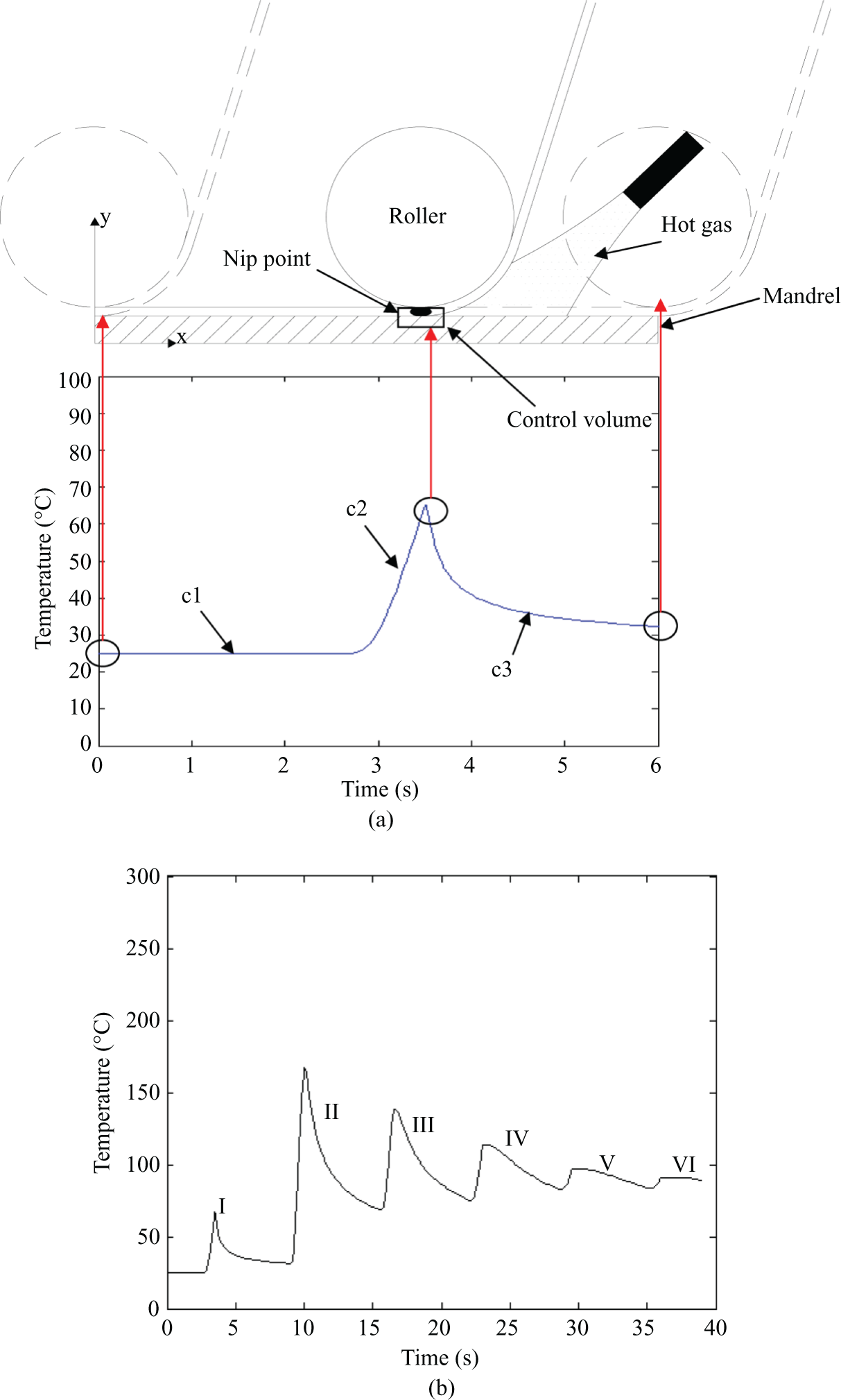
To simplify the simulation, the plate element is chosen. For the simulation of AFP and considering the limitation of computer, each ply is taken as one element in thickness direction, the meshing of mandrel is coarser than that of composite. The boundary conditions of model are shown in Figure 3. The total model has 960 elements, while there are 360 elements for the composite mandrel. The initial temperature is set to 25°C, in the AFP process, both sides and the bottom edge of the mandrel experienced free convection and the temperature of the composite element node is set as 25°C constantly.

Figure 3.

Finite element model and boundary conditions in ANSYS.

Dynamic loading and finite element simulation

The lay-up process is a dynamic process, so composite substrate shape and load distribution change with time. On the one hand, composite substrate grows gradually from bottom to top, from right to left, leading to the number change in the elements. On the other hand, placement head moves at a certain speed along the longitudinal direction of composite material, so the dynamic load should be applied for analysis. These two problems can be successfully resolved using the birth–death element strategy and the cyclic loading strategy in ANSYS. Figure 4 shows the solution procedure. After finishing modelling, all composite elements were deleted and the temperature was maintained at 25°C on their nodes. In the following simulation steps, each loading step was treated as follows:

A larger substep time $t_{i} = t_{i} + Δ t$ is set.

To activate elements step by step to simulate the growth of composite substrate.

To delete the previous step load and apply new load at nodes activated sequentially to simulate the moving of the roller.

Figure 4.

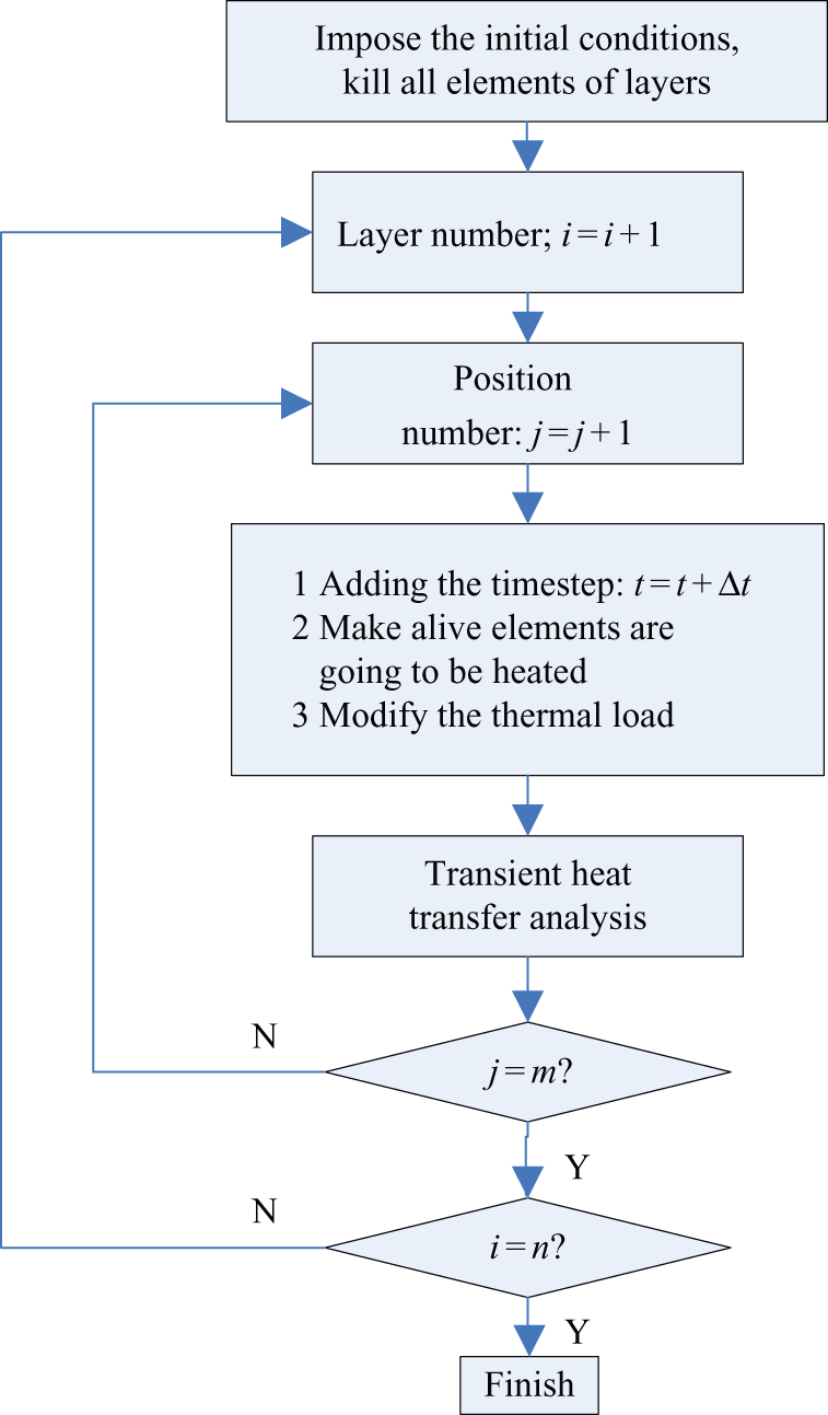
Flow chart for the solution procedure.

The distance between the heater nozzle and the composite substrate is much closer, so the temperature distribution, which can also be called the effective thermal load, of hot gas should be considered uniform. The same convection heat transfer coefficient and temperature were applied on the effective thermal load. Free convection is applied on the other region of the surface of the composite substrate. According to different placement conditions, the length of effective thermal load changes from 0.5 cm to 4.5 cm. In ANSYS, the effective thermal load is equivalent to a forced convection load with the same length, which was 1 cm in the analysis. The length of moving step of effective thermal load is set to be ▵x = 5 mm; therefore, we can get the time step ▵t using the following formula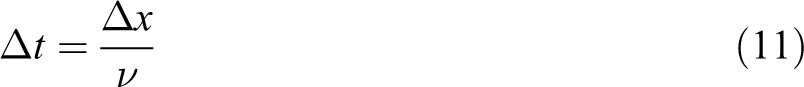

Δ t = \frac{Δ x}{ν}

where ν is the moving speed of roller. Table 3 shows the detailed parameters and boundary conditions.

Table 3.

Parameters and boundary conditions.

Geometry and plies	Single-ply thickness of the prepreg (mm)	0.125
	Mandrel length (mm)	60
	Total number of plies	6
	Thickness of the mandrel (mm)	10
Thermal properties of APC-2	Longitudinal thermal conductivity k_x (W/m°C)	Table 1
	Transverse thermal conductivity k_y (W/m°C)	Table 1
	Density ρ(kg/m³)	1562
	Specific heat c(J/kg°C)	1425
Thermal properties of the mandrel	Thermal conductivity k (W/m°C)	237
	Density ρ(kg/m³)	2700
	Specific heat c(J/kg°C)	905
Boundary conditions	Convective heat transfer coefficients on two sides and bottom of mandrel under free convection h (W/m°C)	13
	Convective heat transfer coefficients of composite under free convection h _free (W/m°C)	13
	Convective heat transfer coefficients of composite under free convection h _force (W/m°C)	Table 2
	Ambient temperature T _∞ (°C)	25
	Initial temperature T ₀ (°C)	25
	Moving speed of roller ν (mm/s)	10
	Temperature of hot gas T _gas (°C)	600

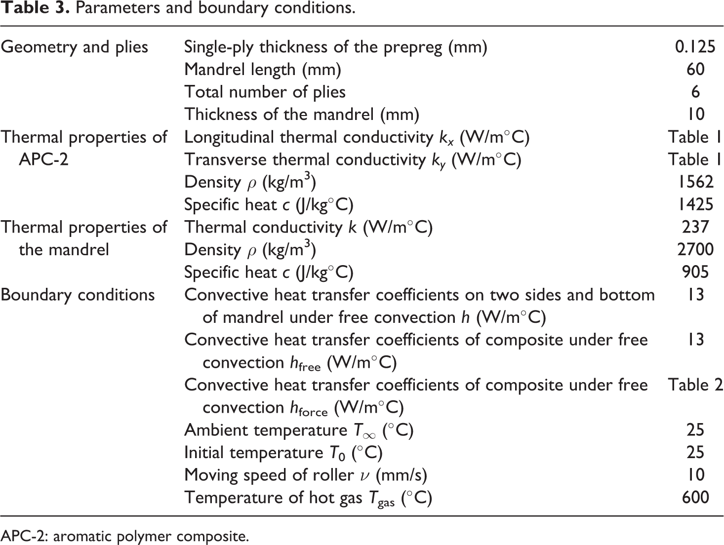
APC-2: aromatic polymer composite.

Figure 5 shows the dynamic changes in temperature field when laying up the first ply. Figure 5(a) to (c) shows the model temperature distribution at 0.5s, 3s and 6.5s, respectively. From the figures, it can be seen that model temperature field changes with the moving of thermal load, composite materials reach the highest temperature when the thermal load moves just above it, and then the temperature reduces slowly after the thermal load moves to the next position on the surface of the composite. Due to the cumulative effect on the temperature, as the lay-up proceeds, the highest temperature increases.

Figure 5.

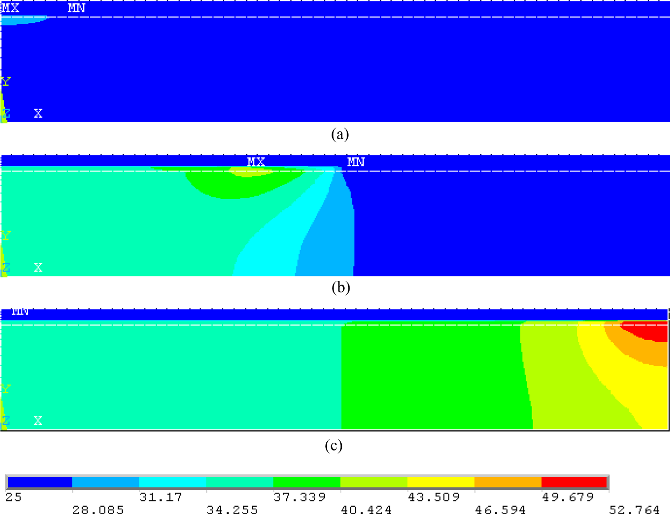
Dynamic changes in the temperature field: (a) temperature distribution at the end of the first load step, (b) temperature distribution when the roller moved to middle of the surface and (c) temperature distribution when the roller moved to the end of the surface.

Simulation results and discussion

Temperature variations in each layer

Nodes are selected on each layer along lay-up direction at 29 mm from the left edge of the model. Numbers of nodes from the first layer to the sixth layer are 273–277, 99. The temperature of node 273, which was considered as the control volume of the transient heat transfer model, in the whole (six) lay-up process, is shown in Figure 6(a).

Figure 6.

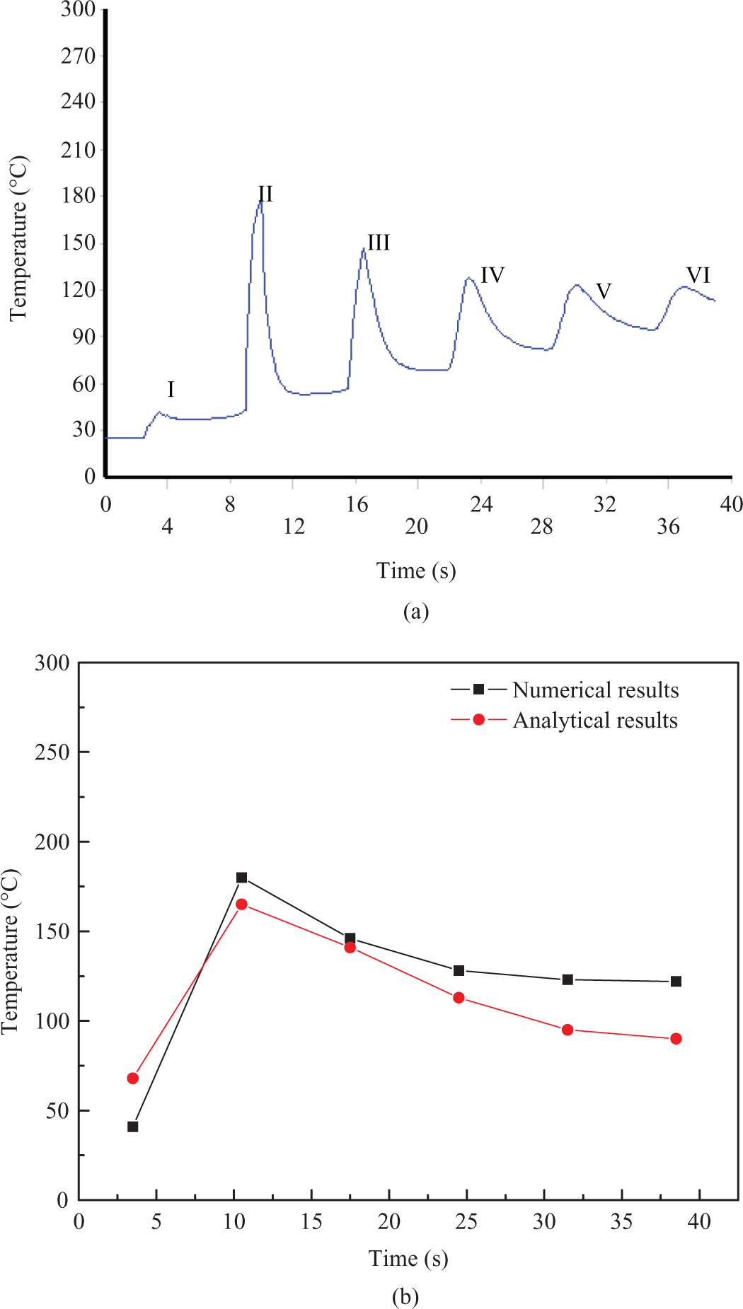
(a) Temperature change at nodes 273 at a heat temperature of 600°C and a moving speed of roller 10 mm/s. (b) Comparison between numerical results and analytical results.

In order to compare the numerical results with the analytical results, each peak temperature of control volume in the first lay-up process, which was calculated by two ways, respectively, is presented in Figure 6(b). It can be found from Figure 6(b) that the numerical results have trends similar to the analytical results shown as follows:

The first peak temperature is much lower than others.

The second peak temperature is the highest.

The temperature decreased gradually from the third peak temperature to the sixth.

Although two curves do not perfectly match due to the impossibility of building an accurate mathematical model, the transient heat transfer model and finite element model can be considered to be comparable.

Temperature of nodes 273–277, 99 in the whole (six) lay-up process is shown in Figure 7. There are six peaks and the nth peak represents node temperature of each layer when the moving heater is above the spot. The first peak is lower because in the lay-up process of the first layer, heat absorption of mandrel is considerable, leading to a slight temperature increase. For the second layer, the first layer is now the composite substrate and the second layer is the prepreg, both of which are welded by hot gas and bonded together; therefore, the temperature of the first layer is close to that of the second layer. It is applicable to the lay-up process from three to six layers. Death and birth of the elements in ANSYS do not mean that elements are removed or built from model, but stiffness matrix of elements is multiplied by a small factor. So node temperature of the second to the sixth layer is set to 25°C in the lay-up process of the first layer.

Figure 7.

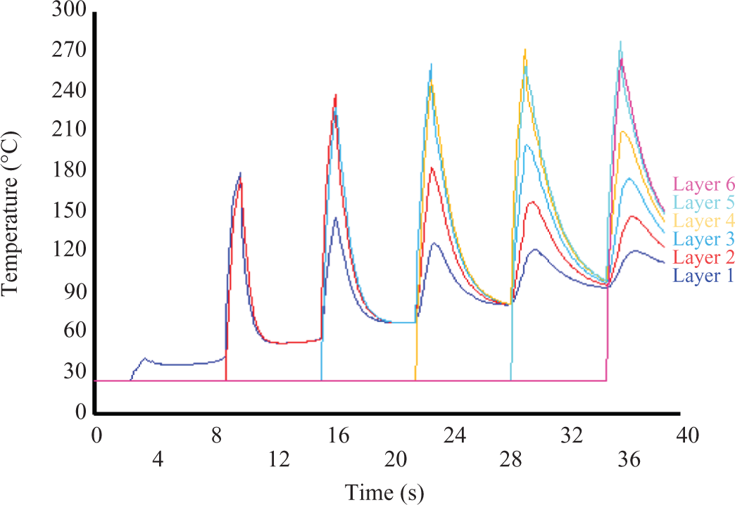
Temperature change at nodes 273–277, 99 at a heat temperature of 600°C and a moving speed of roller 10 mm/s.

The effect of heat temperature on nip point temperature

The heating temperatures of 500°C, 550°C, 650°C, 700°C, 750°C and 800°C are studied. The bonding temperature of each layer is taken as the research object. The results are shown in Figure 8. When the heat temperature rose from 500°C to 800°C, the bonding temperature of each layer increased linearly and its increasing extent is about 100°C. By comparison, the following conclusion could be reached:

The bonding temperature increases linearly with heating temperature.

As the number of layers increases, the increasing rate of bonding temperature decreases.

The temperature difference between the layers decreases with an increase in the number of layers.

Figure 8.

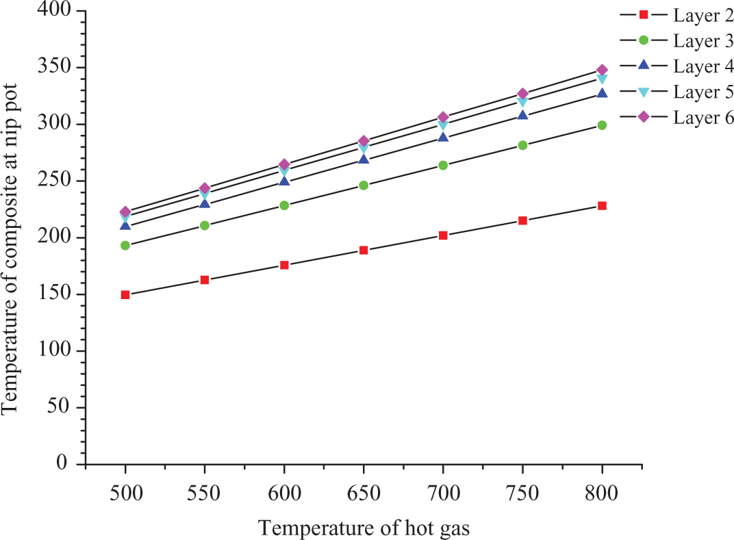
The effect of heat temperature on nip point temperature.

The effect of lay-up speed on nip point temperature

Consider the cases for different lay-up speeds 15 mm/s, 20 mm/s, 25 mm/s, 30 mm/s, 35 mm/s and 40 mm/s with the same heating temperature of 600°C, the bonding temperature on each layer versus the moving speed of roller are obtained after re-simulation. The following conclusions are drawn from Figure 9:

The faster the roller moves, the lower the temperature the nip point of each layer has.

The change in bonding temperature with the moving speed of the roller is non-linear and the bonding temperature changes slowly when the roller moves faster.

Figure 9.

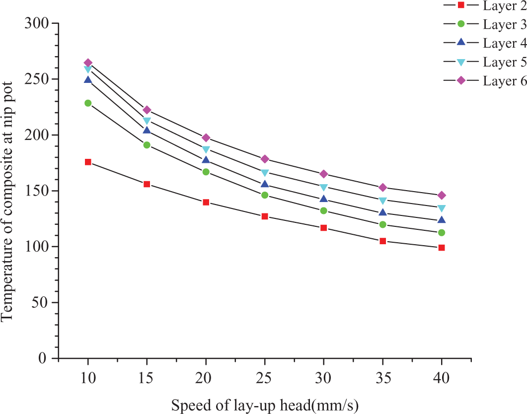
Effect of lay-up speed on nip point temperature.

Conclusions

A semi-infinite solid model was used to analyse the heat transfer in the lay-up process and the heat transfer analysis was conducted (hot gas torch heating) for a lay-up process of thermoplastic matrix composites. The convection coefficients of APC-2 at various temperatures were calculated. The transient temperature field was modelled when the boundary conditions were set as: the temperature of hot gas was 600°C and the moving speed of roller was 10 mm/s.

A dynamic finite element simulation was carried out for the thermoplastic composite tape lay-up process. The birth–death element strategy in ANSYS was used to simulate the movement of lay-up head during dynamic loading and the addition of prepreg onto the composite substrate. Through comparison, the transient heat transfer model and the finite element model can be considered to fit well with each other. The cases of heat temperatures of 500°C, 550°C, 650°C, 700°C, 750°C and 800°C were considered, respectively. The bonding temperature increases linearly with the heating temperature. The cases of lay-up speeds of 15 mm/s, 20 mm/s, 25 mm/s, 30 mm/s, 35 mm/s and 40mm/s were considered, respectively. The faster the roller moves, the lower the temperature the nip point of each layer has. However, the change in bonding temperature with the moving speed of roller is non-linear.

Footnotes

Funding

The financial support from Tianjin Research Program of Application Foundation and Advanced Technology (11JCZDJC23000) is gratefully acknowledged.

References

Ageorges

Hou

. Advances in fusion bonding techniques for joining thermoplastic matrix composites: a review. Composites A 2001; 32: 839–857.

Pitchumani

Ranganathan

Don

. Analysis of transport phenomena governing interfacial bonding and void dynamics during thermoplastic tow-placement. Int J Heat Mass Trans 1996; 39: 1883–1897.

Funck

Neitzel

. Improved thermoplastic tape winding using laser or direct-flame heating. Compos Manuf 1995; 6: 189–192.

Pistora

Yardimci

Guceri

SI.

On-line consolidation of thermoplastic composites using laser scanning. Compos Part A 1999; 30: 1149–1157.

Sonmez

Akbulut

. Process optimization of tape placement for thermoplastic composites. Composites A 2007; 38: 2013–2023.

Sonmez

Hahn

. Analysis of the on-line consolidation process in thermoplastic composite tape placement. J Thermoplast Compos Mater 1997; 6: 543–572.

Yardimci

Pistor

Güçeri

. Process planning for on-line consolidation in tape winding of noncircular thermoplastic composites. J Manuf Processes 2000; 2: 83–99.

Aized

Shirinzadeh

. Robotic fiber placement process analysis and optimization using response surface method. Int J Adv Manuf Technol 2011; 55: 393–404.

Ageorges

Lin

. Simulation of impulse resistance welding for thermoplastic matrix composites. Appl Compos Mater 2001; 8: 133–147.

10.

Mondadori

NML

Nunes

RCR

Canto

. Composites of recycled PET reinforced with short glass fiber. J Thermoplast Compos Mater 2011; 25: 747–764.

11.

Yuan

Zhang

. Experimental investigation on the co-cure processing of honeycomb structure with self-adhesive prepreg. Appl Compos Mater 2008; 15: 47–59.

12.

Wagner

Colton

. On-line consolidation of thermoplastic towpreg composites in filament winding. Polym Compos 2004; 15: 436–441.

13.

Olofsson

. Temperature predictions in thick composite laminates at low cure temperatures. Appl Compos Mater 1997; 4: 1–11.

14.

Tumkor

Turkmen

Chassapis

. Modeling of heat transfer in thermoplastic composite tape lay-up manufacturing. Heat Mass Trans 2001; 28: 49–58.

15.

Guan

Pitchumani

. Modeling of spherulitic crystallization in thermoplastic tow-placement process: heat transfer analysis. Compos Sci Technol 2004; 64: 1123–1134.

16.

Hassan

Thompson

Batra

. A heat transfer analysis of the fiber placement composite manufacturing process. J Reinf Plast Compos 2005; 24: 869–890.

17.

Grove

. Thermal modeling of tape laying with continuous carbon fibre-reinforced thermoplastic. Composites 1988; 19: 367–375.

18.

Kim

Lee

II . A study on heat transfer during thermoplastic composite tape lay-up process. Exp Therm Fluid Sci 1996; 13: 408–418.

19.

Kim

Lee

. Flow and heat transfer analysis during tape layup process of APC-2 prepregs. J Thermoplast Compos Mater 2004; 17:5–12.

20.

Brogan

Monaghan

. Thermal simulation of quartz tube infrared heaters used in the processing of thermoplastic composites. Composites A 1996; 27: 301–306.

21.

Trende

Astrom

Woginger

. Modeling of heat transfer in thermoplastic composites manufacturing: double-belt press lamination. Composites A 1999; 30: 935–943.

22.

Zhao

Hoa

Gao

. Thermal stresses in rings of thermoplastic composites made by automated fiber placement process. Sci Eng Compos Mater 2011; 18: 35–49.

23.

Yunus ACl: Heat transfer. A practical approach. 2nd ed. Beijing, China: Higher Education Press, 2007.

Dynamic finite element simulation and transient temperature field analysis in thermoplastic composite tape lay-up process

Abstract

Keywords

Introduction

Transient temperature field analysis in the thermoplastic composite tape lay-up process

Heat transfer in the lay-up process

Transient temperature field analysis

Dynamic finite element simulation based on ANSYS

Finite element modelling and assumptions

Dynamic loading and finite element simulation

Simulation results and discussion

Temperature variations in each layer

The effect of heat temperature on nip point temperature

The effect of lay-up speed on nip point temperature

Conclusions

Footnotes

Funding

References