Optimization of thermoplastic composites resistance welding parameters based on transient heat transfer finite element modeling

Abstract

The use of resistance welding technology to join thermoplastic composite aerospace structures is still contingent upon a better understanding of the heat transfer mechanisms occurring during welding, which govern the joint quality and mechanical performance. In this study, two-dimensional (2D) and three-dimensional (3D) transient heat transfer finite element models were developed to simulate resistance welding of thermoplastic composites. The 2D model was used to investigate the effect of the length of the exposed areas of the heating element to air (clamping distance) on the local overheating at the edges and the effects of the input power level on the thermal behavior of the welds. It is shown that controlling the clamping distance improves the thermal uniformity of the weld. The 3D model shows that heat conduction along the length of the laminates influences the thermal uniformity of the weld interface. An optimization chart is developed in order to minimize the undesirable edge effect and to define the conditions required to obtain a complete weld. The results of the 3D model are compared with experimental data.

Introduction

Thermoplastic matrix composites, which offer the possibility of being reprocessed, can be joined by fusion bonding. Fusion bonding or welding consists of heating the polymer at the interface of two laminates to be joined, physically causing polymer chains interdiffusion, and then cooling the polymer to consolidate the joint. The heat at the interface can be generated by means of direct input of heat, frictional work, electrical current or electromagnetic field. Resistance welding has been identified as a fast process that requires little to no surface preparation and can be applied to all thermoplastic polymers. ^1,2 In addition, the simple and inexpensive welding equipment can be designed to be portable for repair purposes. ¹ Resistance welding consists of heating the interface of the parts to be joined by passing an electrical current through a resistive implant called heating element. The temperature of the heating element increases by Joule heating, causing the surrounding polymer to soften or melt. The polymer then diffuses through the heating element and cools down and consolidates under an applied pressure to form a weld. ¹

The resistance welding process has been studied numerically and experimentally. Several issues such as overheating of the edges of the weld, nonuniform temperature distribution at the weld interface and inconsistent weld performance, quality and strength have been reported. ^{3 –5} These issues were particularly important when carbon fiber heating elements were used. ⁶ The introduction of stainless steel mesh heating elements recently improved the weld performance and consistency with lap shear strengths up to 50 MPa for unidirectional carbon fiber/polyether-ether-ketone ([PEEK] APC-2/AS4), carbon fiber/polyether-ketone-ketone and carbon fiber/polyether-imide adherends welded with an optimum heating element mesh size. ^7,8 However, the nonuniform temperature distribution at the weld interface remains an issue.

Thermal analysis can be used to determine the thermal insulation, input energy and heating time required for a high-quality bond. Xiao et al. ⁹ used finite element modeling to show that a good thermal insulation and a correct amount of input energy can reduce the welding time and enhance weld quality. Ageorges et al. ^{10 –12} and Holmes and Gillespie ¹³ showed that the heat generated by the part of the heating element that is inside the weld is rapidly transferred by conduction to the polymer and laminates, whereas the heat in the parts that are exposed to air can only be transferred by radiation and free convection with a much slower speed. This difference in heat transfer mechanisms between the center and the edge of the weld seems to be responsible for a nonuniform heating at the weld interface and has been referred to as “edge effect” in the literature. ¹ Experimental investigations showed that the position of the electrical connectors with respect to the weld stack, that is, clamping distance, has a significant influence on the edge effect. ^2,14,15

The objective of this article is to demonstrate how the clamping distance affects the heat distribution in the weld and how it can be controlled to improve temperature uniformity. To do so, two-dimensional (2D) and three-dimensional (3D) finite element models are built and used to investigate temperature profiles under various input power levels and clamping distances. An optimization chart is proposed to minimize the undesirable edge effect and to define the conditions required to obtain a complete weld. Finally, the results of the 3D model are compared with experimental data. The main objective of this work is to provide complete understanding of the resistance welding process for the development of resistance-welded thermoplastic composite structures in the next generation of aircrafts.

Resistance welding setup and materials

Figure 1 shows a schematic of the resistance welding setup for a lap shear joint. The setup consists of a weld stack, a DC electrical power supply, a pressure system and a resistance welding rig. The rig consists of copper electrical connectors and ceramic sample holders and insulators. The adherends to be welded consist of 16 plies of unidirectional APC-2/AS4 composite laminates. The glass transition and melting temperatures of PEEK are 143°C and 343°C, respectively. The adherends are 101.6 mm long in the fiber direction, 25.4 mm wide and 2.16 mm thick. The overlap width of the weld is 12.7 mm. The heating element consists of a 0.08-mm thick plain weave stainless steel mesh made of 0.04-mm diameter wires with a 0.09-mm open gap width. The heating element is sandwiched between two 0.127 mm thick neat PEEK polymer films. The ends of the heating element are connected to the DC power supply using copper electrical connectors. The weld stack is insulated on top and bottom with 37.5 mm thick Wonderstone alumina silicate ceramic plates.

Figure 1.

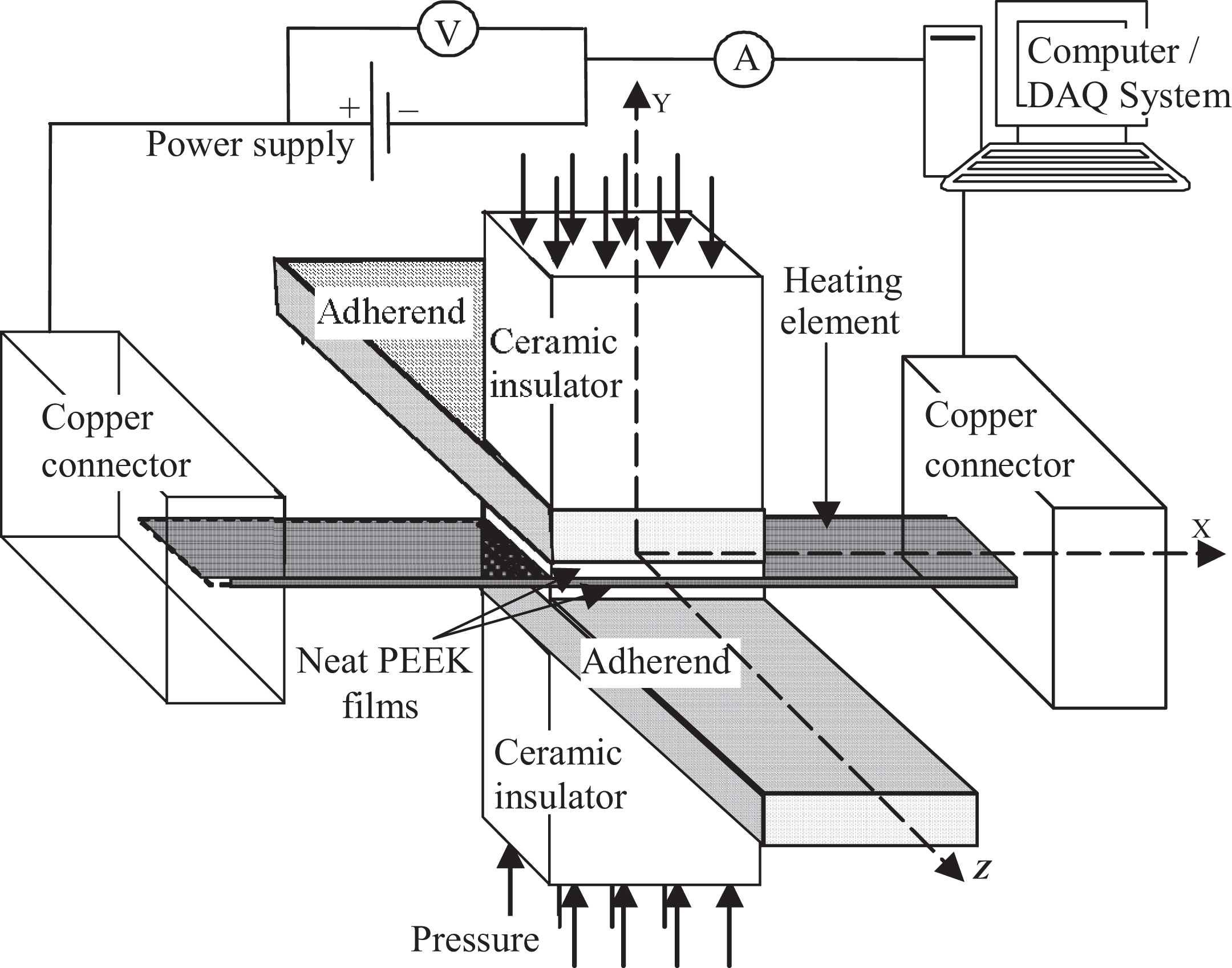
Schematic representation of resistance welding. ¹⁶

Models development

Both 2D and 3D heat transfer finite element models were developed using ANSYS 8.0 finite element software. In order to simplify the model and reduce the computational time, the following assumptions were made:

1. The pressure and small displacements of the laminates are neglected.

2. The process is modeled as a heat transfer problem only. Therefore, the flow of melted polymer out of the weld, due to the applied pressure, is neglected.

3. A constant volumetric power density (HGEN) $\dot{q}$ is applied to the heating element to account for Joule heating, calculated with $\dot{q}=R\cdot I^2/U$ , where q is the volumetric power density (W/m³), R is the electrical resistance (Ω) of the heating element, I is the applied current (A) and U is the volume of the heating element (m³).

4. A constant thermal convection coefficient h _air = 5 W/m² K and temperature T_∞ = 20°C is assumed for the surrounding air.¹³

5. The heating element is assumed to behave as a gray-body radiating object with an emissivity ε = 0.95 and the Stefan-Boltzmann constant σ = 5.67 × 10⁻⁸ W/m² K.¹⁷

6. The latent heat of fusion of the polymer is neglected. ^10,12,13

Finite element models

The 2D transient heat transfer finite element model simulates the temperature gradient along the width of the weld, that is, the X direction (Figure 2). To reduce the computational time, symmetric boundary conditions, that is, zero heat flux, are applied on the X-Z and Y-Z planes. Orthotropic material properties are applied. The 3D model investigates the effect of heat conduction along the length of the laminates (Figure 3). In order to better represent the experimental setup, all of the ceramic blocks are modeled. Zero heat flux boundary conditions are applied on the Y-Z plane. Convergence study was performed on the obtained results with a convergence criterion of 5%.

Figure 2.

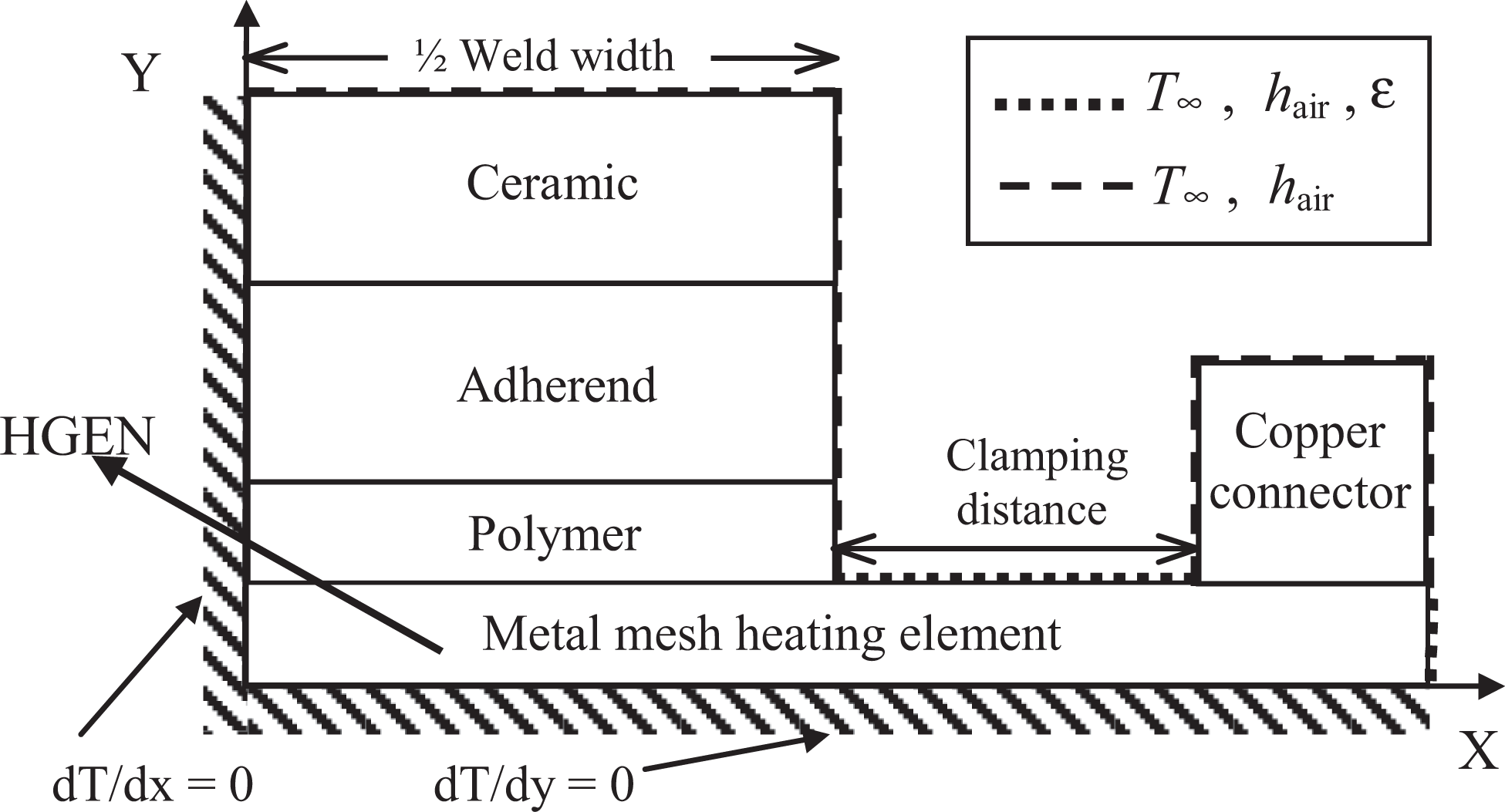
Two-dimensional model definition (not to scale). T _∞ is the ambient temperature (20°C), h _air is the convection coefficient (5 W/m² K), and ε is the emissivity (0.95).

Figure 3.

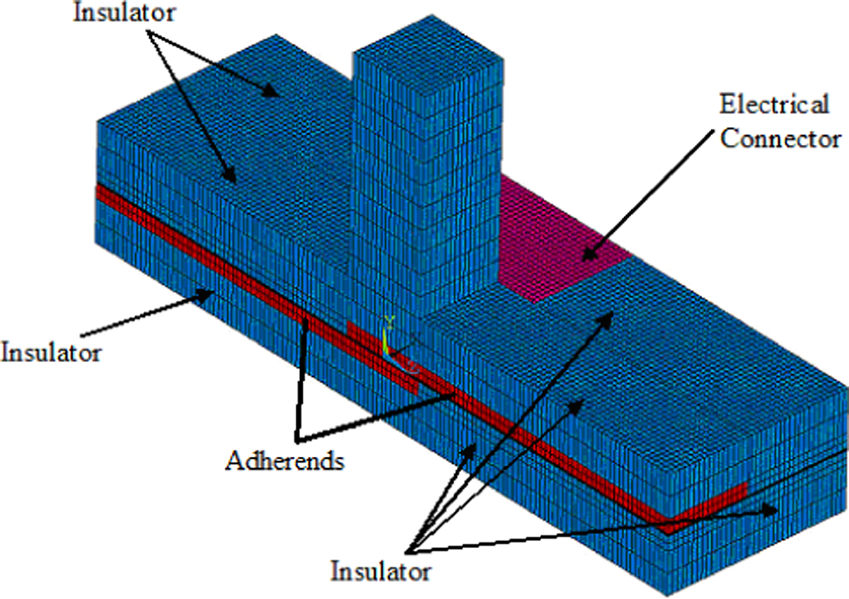
Three-dimensional finite element model.

Materials properties

The required properties to input for each material are the density, specific heat or enthalpy and thermal conductivity. For orthotropic materials, such as composite materials, the thermal conductivity tensor is diagonal and the heat diffusion equation is:

$\left(k_{xx}\frac{{\mathrm{\partial }}^{2}T}{\mathrm{\partial }{x}^2}+k_{yy}\frac{{\mathrm{\partial }}^{2}T}{\mathrm{\partial }{y}^2}+k_{zz}\frac{{\mathrm{\partial }}^{2}T}{\mathrm{\partial }{z}^2}\right)+\dot{q}=\mathit{\rho }\cdot c_p\frac{\mathrm{\partial }T}{\mathrm{\partial }t}$

1

where x, y and z are the Cartesian coordinates, T is the temperature, t is the time, ρ is the density, c_p is the specific heat, k_xx , k_yy and k_zz are the thermal conductivities in the x, y and z directions, respectively, and $\dot{q}$ is the volumetric heat source term in the heating element. Table 1 presents the room temperature material properties of the APC-2/AS4 laminate, stainless steel mesh, PEEK film, copper connector and ceramic tooling plates. ^{18 –21} Since the PEEK specific heat and density vary with temperature, temperature-dependant values are considered in the analysis (Table 2). All other quantities are considered temperature independent.

Table 1.

Thermal properties at room temperature. ^{17 –20}

Material properties	APC-2/AS4 laminate	Metal mesh	APC-2 film	Copper	Ceramic
kxx (W/m°C)	0.658	2.18	0.25	345	1.26
kyy (W/m°C)	0.658	0.21	0.25	345	1.26
kzz (W/m°C)	6.8	2.18	0.25	345	1.26
Density (kg/m3)	1598	2973	1298	8900	2715
Specific heat (J/kg°C)	930	735	944	385	1000

Table 2.

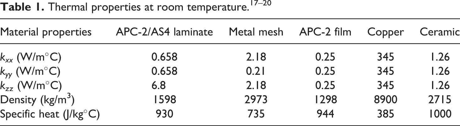
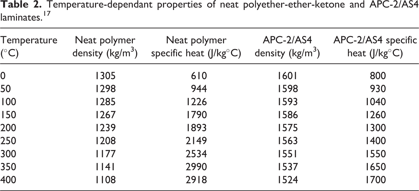
Temperature-dependant properties of neat polyether-ether-ketone and APC-2/AS4 laminates.¹⁷

Temperature (°C)	Neat polymer density (kg/m3)	Neat polymer specific heat (J/kg°C)	APC-2/AS4 density (kg/m3)	APC-2/AS4 specific heat (J/kg°C)
0	1305	610	1601	800
50	1298	944	1598	930
100	1285	1226	1593	1040
150	1267	1790	1586	1260
200	1239	1893	1575	1300
250	1208	2149	1563	1400
300	1177	2534	1551	1550
350	1141	2990	1537	1650
400	1108	2918	1524	1700

The heating element is considered to be a single cross ply layer. Its effective thermal conductivities (x, y and z directions) are calculated as proposed by Xu and Wirtz. ²² The effective specific heat and density of the heating element, which are considered constant with temperature, are calculated using the rule of mixture as shown in equations (2) and (3):

${\mathit{\rho }}_{\text{heating element}}={\mathit{\rho }}_{\text{steel}}\cdot v_{\text{steel}}+{\mathit{\rho }}_{\text{PEEK}}\cdot v_{\text{PEEK}}$

2

$C_{p\text{heating element}}=\frac{{\rho }_{\text{steel}}.v_{\text{steel}}.c_{p\text{steel}}+{\rho }_{\text{PEEK}}.v_{\text{PEEK}}.c_{p\text{PEEK}}}{{\rho }_{\text{heating element}}}$

3

where υ is the volume fraction of the constituent.

Modeling results and discussion

In this section, the influences of the welding time and input power level on the thermal history of the weld are addressed. In order to facilitate the description of the observed phenomena, the following definitions must be clarified.

1. The processing temperature of PEEK is 390°C.

2. The minimum welding time is the time required to reach 343°C, the PEEK melting temperature, ‘everywhere’ at the weld interface, so that the entire weld interface is melted.

3. The maximum welding time is the time required to reach 450°C, the PEEK degradation temperature, ‘anywhere’ at the weld interface, in order to avoid degradation at any location in the weld.

4. The processing window is the difference between the maximum welding time and the minimum welding time.

5. A complete weld is obtained when all temperatures at the weld interface are between the maximum and minimum welding temperatures, that is, 450°C and 343°C, respectively.

6. The weld interface is the surface between the laminate and the PEEK film.

7. The clamping distance is defined as the distance between the edge of the weld and the copper electrical connector, as shown in Figure 2.

Local overheating issue

The 2D model is used to investigate the edge effect, that is, overheating of the edges of the weld, due to the areas of the heating element exposed to air. Figure 4 shows the temperature distribution along the weld interface after a fixed input power level of 2.0 GW/m³ is applied to the heating element for 10 seconds, 20 seconds, 30 seconds and 40 seconds. The results of Figure 4 clearly show that the temperature at the edges of the weld is substantially higher than the temperature inside the weld. After 10 seconds, the temperature at the edge of the weld rapidly reaches 360°C, whereas the temperature at the center of the weld is only 260°C. After 20 seconds, the edges of the weld interface have already reached the polymer degradation temperature of 450°C, whereas the center of the weld has risen just above the melting temperature of the polymer (343°C). It is clear that such temperature gradient cannot be tolerated in the manufacturing environment for producing thermoplastic composite structures, for example, welding stringers to skin. Moreover, the melt front has already started to propagate through the weld thickness, at the edges of the weld. This would experimentally cause fiber motion and squeeze out of the resin. After 30 seconds, the entire weld interface is well above 343°C, but the region of degraded polymer is growing at the edges. After 40 seconds, the polymer at the weld interface is assumed to be entirely degraded, since the temperature at the weld interface is equal or superior to 450°C everywhere.

Figure 4.

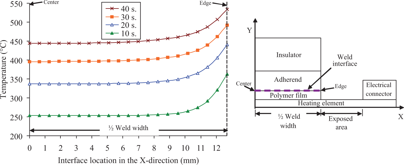
Predicted temperature profile along the weld interface for a power level of 2.0 GW/m³, using the 2D model. 2D: two-dimensional.

As seen in the previous figure, the problem of local overheating arises from sudden change of heat transfer mechanisms from conduction to convection and radiation at the edges of the weld. The areas of the heating element exposed to air have poor heat transfer properties due to free convection. Hence, the exposed areas reach a higher temperature faster than the areas of the heating element in contact with the weld interface. Cooling the edges, insulating the exposed areas or reducing the clamping distance are possible solutions to reduce the sharp temperature gradient at the edges of the weld. These methods can add additional variables in the process, which may lead to unrepeatable and unreliable results, if they are not controlled thoroughly. Understanding the effects of the variables is essential to obtaining good weld quality. In particular, the effect of the clamping distance on the temperature uniformity must be understood. It is believed that an optimum clamping distance can offer a uniform temperature distribution in the weld. Here, it is important to recall that a complete weld can only be produced once the temperatures at the weld interface are between the polymer melting and degradation temperatures, that is, 343°C and 450°C, respectively. However, to improve weld quality, it is needed to have a uniform temperature distribution at the weld interface. In order to determine this optimum clamping distance, an optimization algorithm is incorporated in the 2D heat transfer finite element model. The objective is to reach a processing temperature of 390°C everywhere along the width of the weld by varying the clamping distance. This objective function is schematized as follows:

$\mathrm{M}\mathrm{i}\mathrm{n}\left(f(T)\right)=\mathrm{M}\mathrm{i}\mathrm{n}\left(\left|T_{\mathrm{c}\mathrm{e}\mathrm{n}\mathrm{t}\mathrm{e}\mathrm{r}}-T_{\mathrm{e}\mathrm{d}\mathrm{g}\mathrm{e}}\right|\right)$

12

with T _center = 390°C; where T _center is the temperature at the center of the weld and T _edge is the temperature at the edge of the weld. Figure 5 shows the bisection algorithm applying the objective function.

Figure 5.

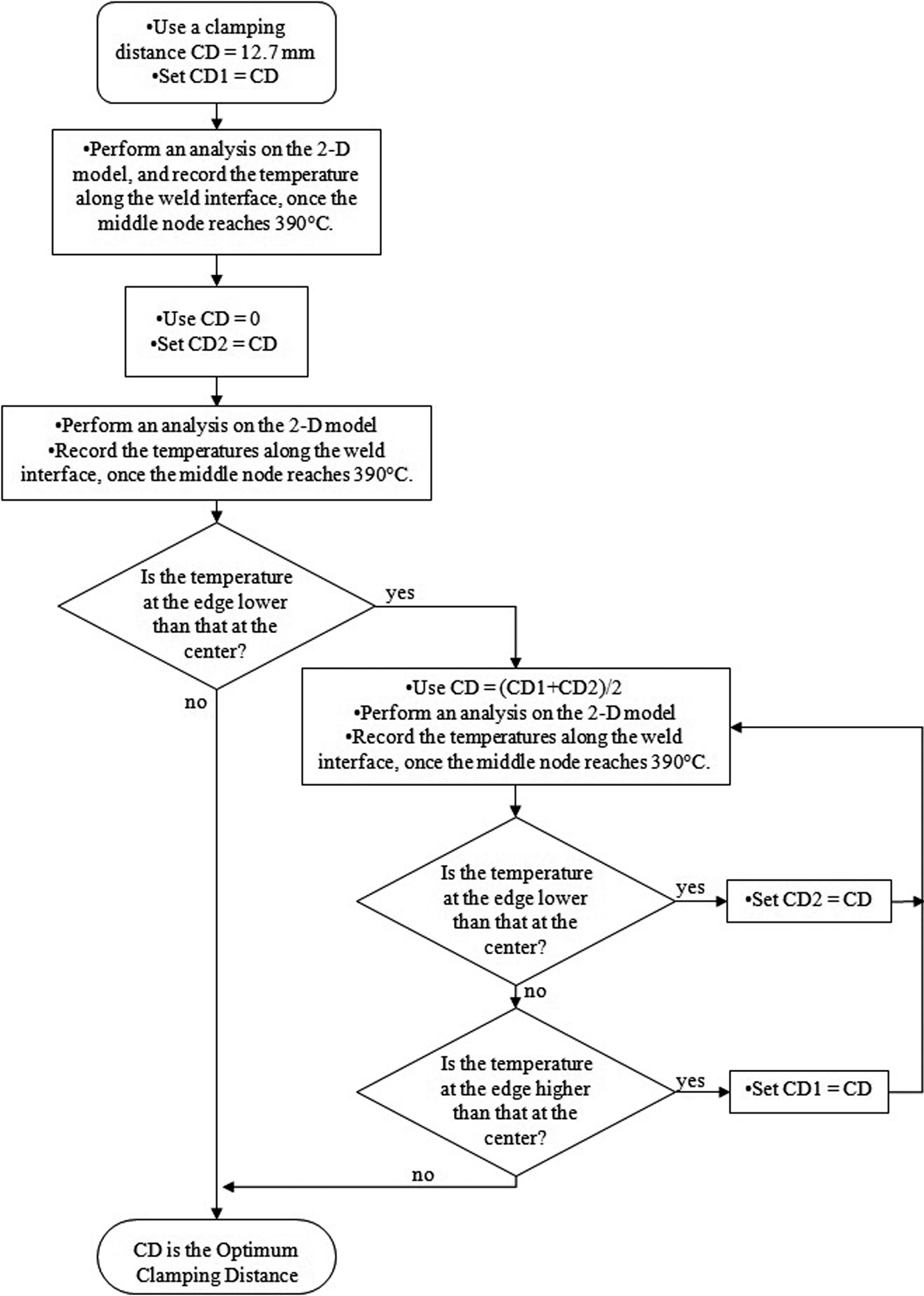
Chart showing clamping distance optimization.

Figure 6 shows the temperature distribution along the width of the weld interface for different clamping distances and a constant power level of 2.0 GW/m³ applied during 29 seconds. From this figure, it can be seen that a zero clamping distance, far from solving the edge effect issue, instead promotes excessive heat dissipation into the electrical copper connectors by conduction, which leads to cold edges and unwelded zones at the edges of the weld. Figure 6 also shows that the optimum clamping distance for a constant power level of 2.0 GW/m³ is 0.65 mm. In effect, a clamping distance of 0.65 mm leads to an almost uniform temperature over the width of the weld. The implications of this optimization are shown in Figure 7 and Figure 8, where the thermal history at the weld interface for two clamping distances, that is, 12.7 mm and 0.65 mm, is depicted. In both cases, the thermal history is studied for 50 seconds of applied power. The transient temperature profiles at different locations across the width of the weld, that is, at 0 mm (center), 9.5 mm, 11.1 mm and 12.7 mm (edge), are presented. For the clamping distance of 12.7 mm, the obtained processing window for a complete weld is only 0.5 second, ranging from 21 seconds to 21.5 seconds. Decreasing the welding time below 21 seconds leads to an unwelded zone at the center of the weld, while increasing the welding time above 21.5 seconds causes polymer degradation and local overheating at the edges of the weld, due to the large clamping distance of 12.7 mm. For the optimum clamping distance of 0.65 mm, the processing window for a complete weld is 20.5 seconds, ranging from 21 seconds to 41.5 seconds, as shown in Figure 8. This clearly shows that using an appropriate clamping distance can provide a more uniform temperature distribution across the weld and significantly enlarge the size of the processing window. The optimum clamping distance that allows the heating element to cool down properly while permitting the center of the weld to reach the minimum melting temperature of 343°C is responsible for this better and reasonable processing window. This large processing window facilitates the control of the welding process and may lead to more uniform temperature and thus better weld quality.

Figure 6.

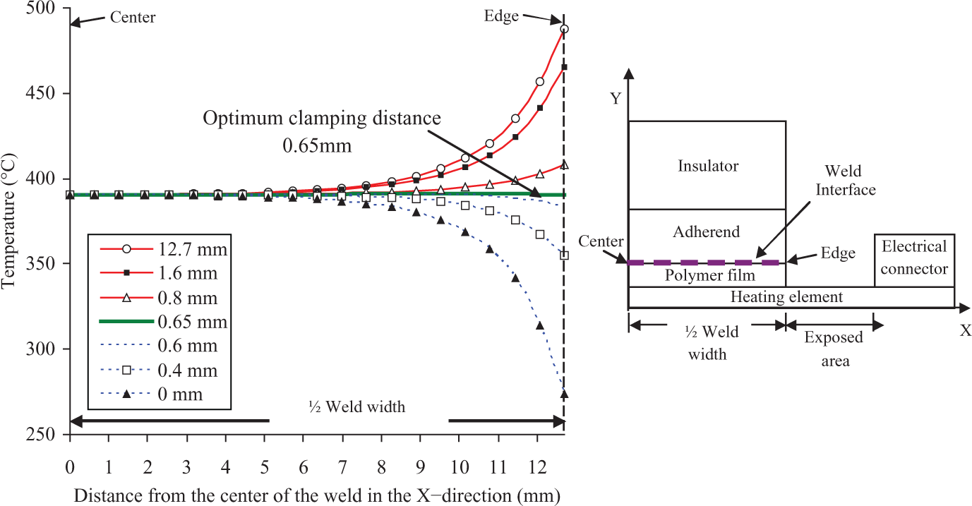
Effect of the clamping distance on local overheating (2D model). 2D: two-dimensional.

Figure 7.

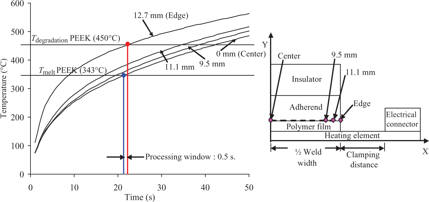
Predicted thermal history at various locations in the weld for a clamping distance of 12.7 mm at a power level of 2.0 GW/m³ using the 2D model. 2D: two-dimensional.

Figure 8.

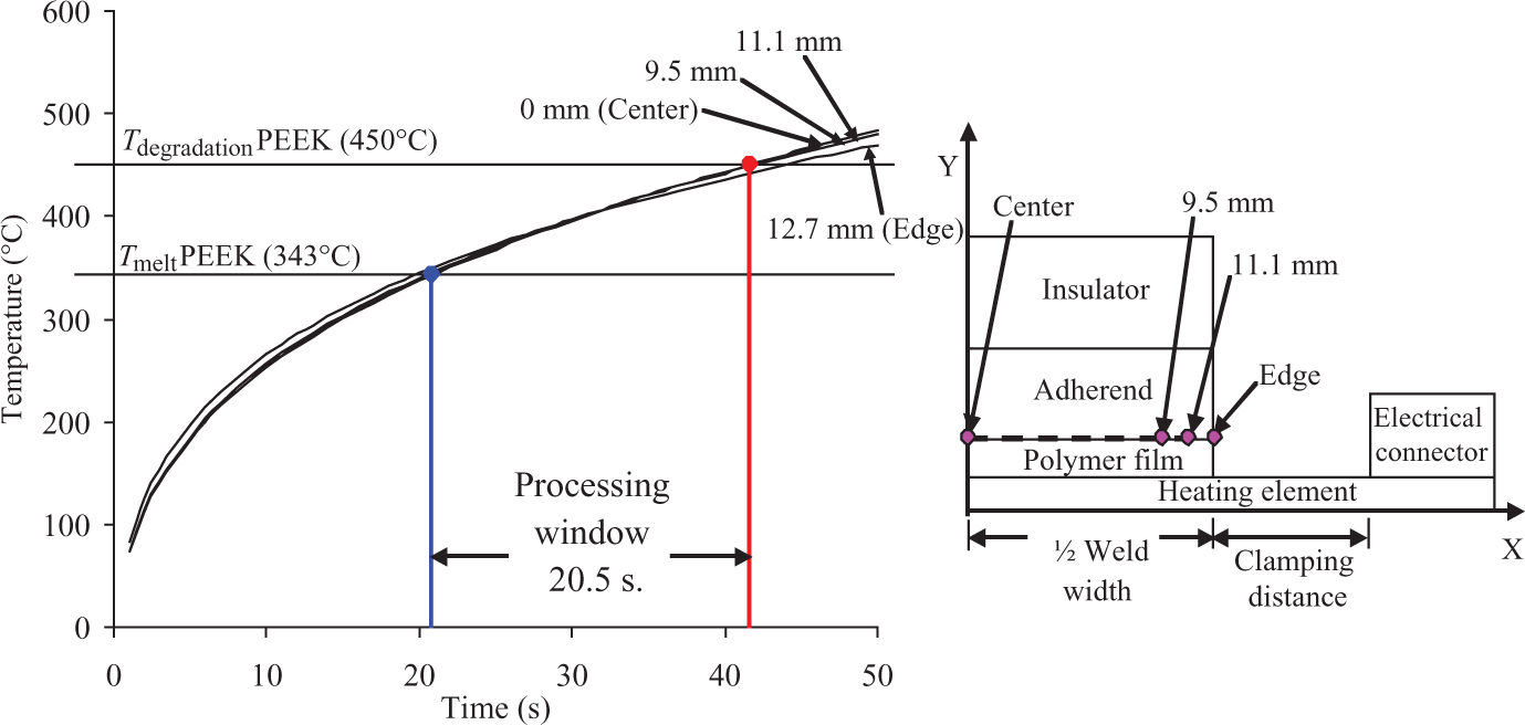
Predicted thermal history at various locations in the weld for a clamping distance of 0.65 mm at a power level of 2.0 GW/m³ using the 2D model. 2D: two-dimensional.

Effect of power level

The 2D model is also used to investigate the influence of various power levels on the welding times. Table 3 shows the minimum and maximum welding times, as well as the size of the processing windows for the 1.0 GW/m³, 1.5 GW/m³, 2.0 GW/m³ and 2.5 GW/m³ applied power levels and the clamping distances of 12.7 mm, 0.65 mm and 0 mm. In this table, a negative processing window means that the polymer degrades at some places in the weld before the polymer is melted everywhere over the weld area. Therefore, a negative processing window means no processing window exists for this particular set of welding parameters.

Table 3.

Processing windows for different clamping distances and power levels.

Power (GW/m3)	Minimum welding time (s)	Maximum welding time (s)	Processing window (s)
Clamping distance = 12.7 mm
1.0	43	53	10
1.5	28.5	31.5	3
2.0	21	21.5	0.5
2.5	14.8	14	−0.8
Clamping distance = 0.65 mm
1.0	46.5	87.5	41
1.5	28.5	57	28.5
2.0	21	41.5	20.5
2.5	15.2	30	14.8
Clamping distance = 0 mm
1.0	112	88	−24
1.5	72	57	−15
2.0	52	41.5	−10.5
2.5	18.8	14.7	−4.1

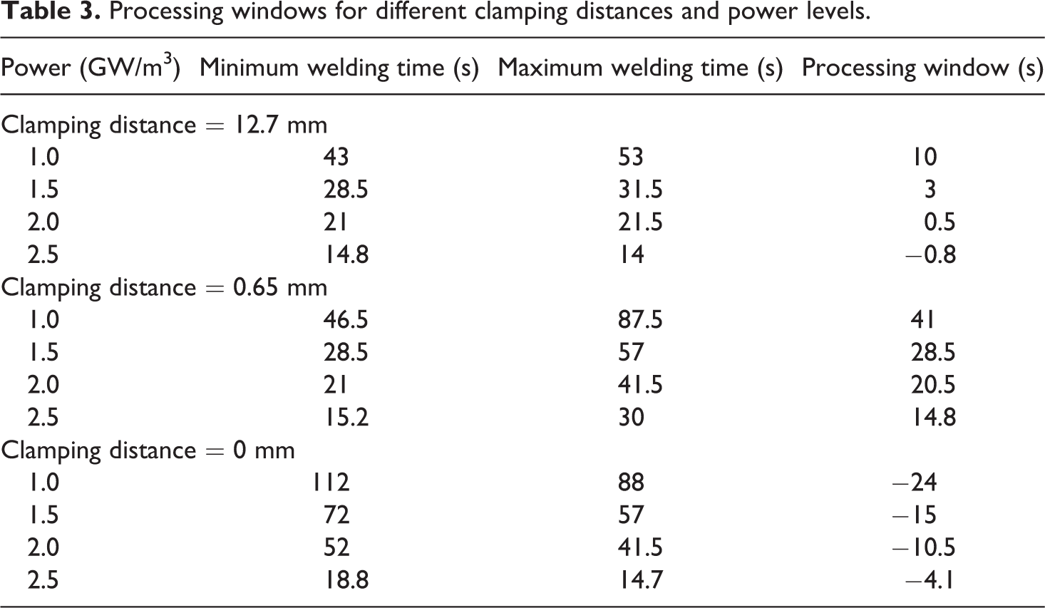
For a clamping distance of 12.7 mm and power level of 2.5 GW/m³, a negative processing window is obtained, meaning that under these conditions, polymer degradation at the edges of the weld occurs before the polymer at the center of the weld reaches the melting temperature. Therefore, no complete weld is possible at any welding time. For the same clamping distance, the lowest power of 1.0 GW/m³ provides the largest processing window of 10 seconds. The drawback of this low power level is a long welding time of 43 seconds, causing melt front propagation through the weld thickness, which in turn promotes fiber movement at the weld interface. For the 0.65 mm clamping distance, the size of the processing window can be expanded for all power levels, even for the highest power of 2.5 GW/m³, where the processing window expanded from 0 to 14.8 seconds. However, when the clamping distance is reduced to 0 mm, the processing windows are negative for all power levels, meaning that no weld is possible, at any welding time. Therefore, adjusting the clamping distance can significantly improve the size of the processing window especially for the higher power levels.

Heat transfer along the length of the laminates

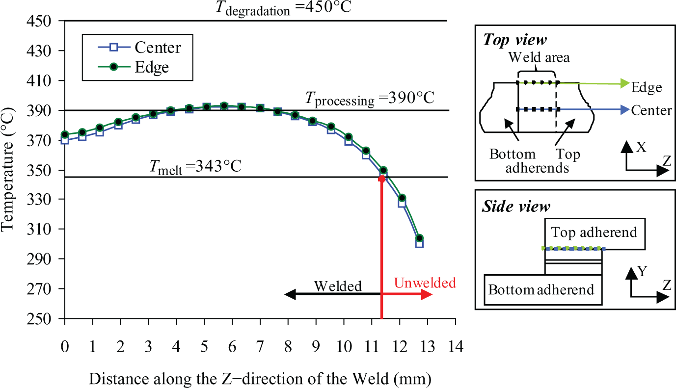
The 3D model is used to provide additional insight during the resistance welding process, taking into account the heat transferred along the laminates. Figure 9 shows the weld interface temperature distributions along the Z direction at the edge and center of the weld for a power level of 2.0 GW/m³, a clamping distance of 0.65 mm and a processing temperature of 390°C. The welding simulation is terminated after 43 seconds, which is the time required for the processing temperature to be reached at the center of the weld interface. This welding time of 43 seconds is different from the 29 seconds obtained with the 2D model and the temperature curves at the edge and at the center of the weld do not lie on top of each other. The increased heating time is due to the heat conduction along the length of the laminates, which influences the temperature distribution over the weld area. This indicates that a 3D model is necessary to determine the thermal behavior of the weld and to optimize the clamping distance.

Figure 9.

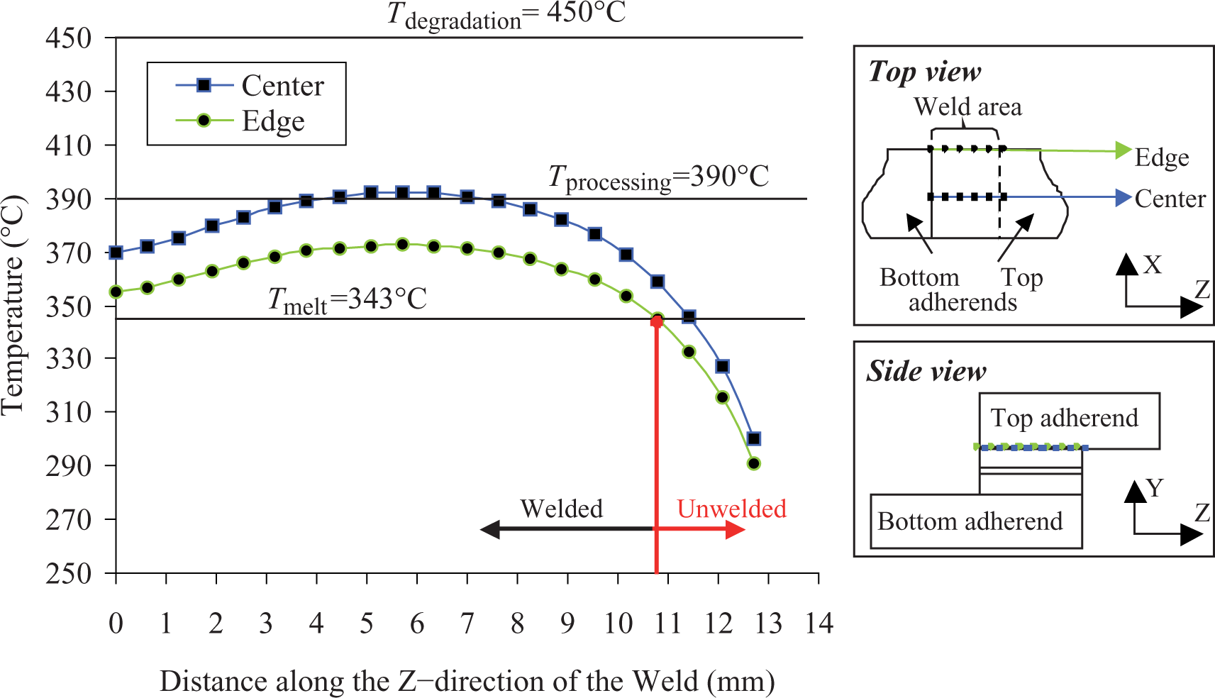
Predicted temperature profile along the length of the weld for an input power level of 2.0 GW/m³ for 43 seconds and a clamping distance of 0.65 mm using the 3D model. 3D: three-dimensional.

The 3D model is coupled with the optimization algorithm shown in Figure 5 and leads to a new optimum clamping distance of 0.8 mm. Figure 10 shows the weld interface temperature distributions along the Z direction at the edge and center of the weld for the power level of 2.0 GW/m³, the clamping distance of 0.8 mm and the processing temperature of 390°C. A combination of welded and unwelded zones, that is, an incomplete weld, can be identified. The nonuniform temperature distributions are attributed to the heat transfer into the laminates along the Z direction. To obtain a complete weld, one possible solution is to increase the processing temperature from 390°C to 440°C. Figure 11 depicts the temperature distributions along the Z direction at the edge and center of the weld for the processing temperature of 440°C. A complete weld is finally achieved in this case. However, it is possible to observe that a nonoptimal clamping distance would bring the curves further apart, causing unwelded zones or degraded zones. Also, it shows that the processing window for this power level is very small, since a small variation in the welding time could cause unwelded or degraded/overheated zones. Finally, Figure 11 shows that it is impossible to obtain a uniform temperature distribution at the weld interface for the current resistance-welded lap shear joint configuration. However, despite having nonuniform heating, a complete weld can be achieved. These conclusions can have influence on the design for manufacturing of resistance-welded thermoplastic composite aerospace structures, where large components need to be assembled. Modeling of larger weld area will have to be conducted in order to design a resistance welding setup capable of improving temperature uniformity over large areas.

Figure 10.

Predicted temperature profile along the length of the weld for an input power level of 2.0 GW/m³ for 43 seconds and a clamping distance of 0.8 mm using the 3D model. 3D: three-dimensional.

Figure 11.

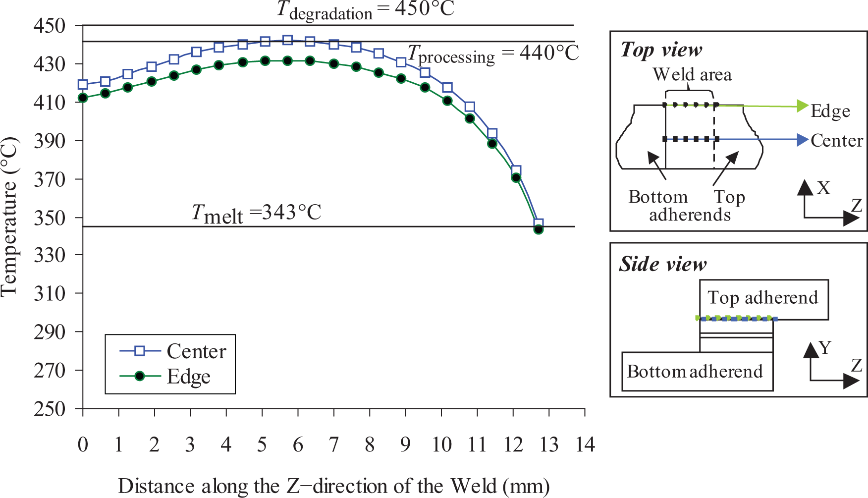
Predicted temperature profile along the length of the weld for an input power level of 2.0 GW/m³ for 61 seconds and a clamping distance of 0.8 mm using the 3D model. 3D: three-dimensional.

Experimental validation

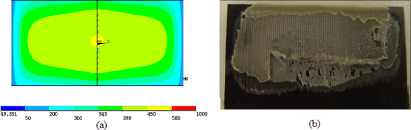
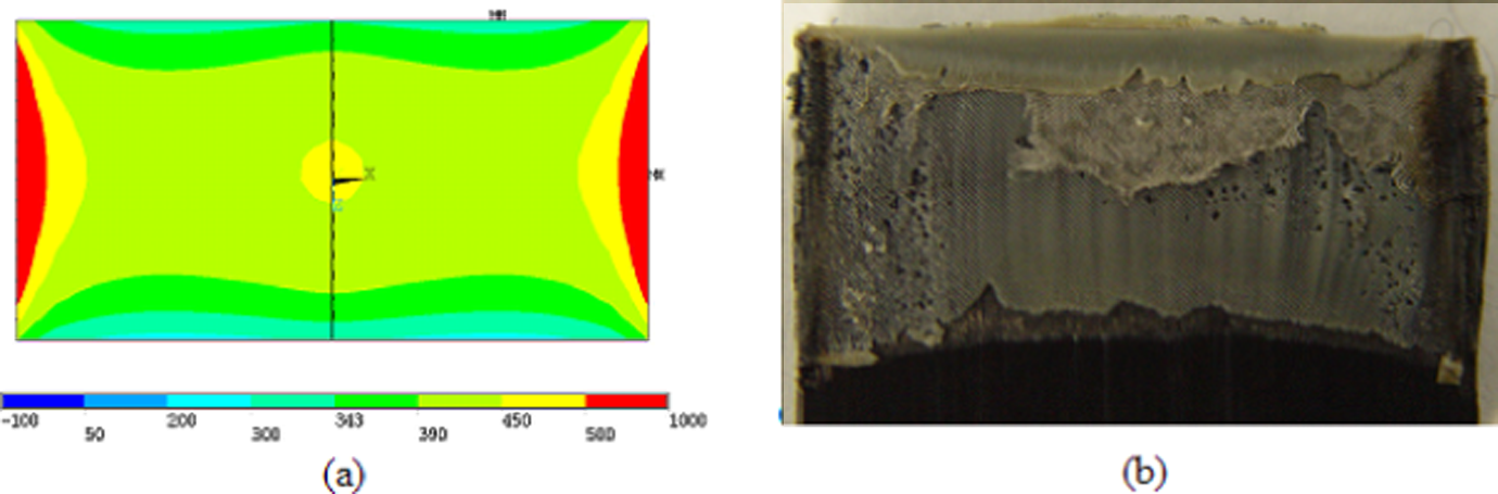
In order to validate the modeling results, welds were performed experimentally. To do so, a constant voltage of 6.0 V, corresponding to a power density of 2.0 GW/m³, is applied to the heating element using a DC power supply. Once the desired processing temperature is reached, the voltage is stopped and the weld is allowed to cool down, under an applied pressure of 1.0 MPa. Two processing temperatures of 390°C and 440°C are compared using an optimum clamping distance of 0.8 mm, as determined in the previous section. Then, the effect of the clamping distance is verified, using three clamping distances of 3.2 mm, 0.8 mm and 0 mm, at the optimum processing temperature of 440°C. This implies four different welding conditions. Three samples were welded for each condition. Afterward, the samples were mechanically tested, using the ASTM D1002 standard, in order to compare their lap shear strengths. The following four figures show the weld interface of the average lap shear strength sample welded under these conditions next to the numerically obtained temperature contours, for each condition. Figure 12 and 13 show that the model predicts adequately the evolution of temperature distribution through the weld thickness. The black areas on each side of the weld show that the heating element is oxidized due to the contact with air during heating. The numerical and experimental temperature distributions at the weld interface matches, showing a brighter color at the weld interface of the welded samples. Comparing Figures 12 and 13, we can confirm that increasing the processing temperature, as well as the welding time, increases the welded area. In effect, Figure 13(b) shows a larger region of melted polymer when compared with Figure 12(b), where the unmelted polymer is visible. Moreover, as seen in Table 4, the processing temperature of 440°C led to the best mechanical performance, which is in agreement with the numerical results, that is, indication of a complete weld across all the joint areas.

Figure 12.

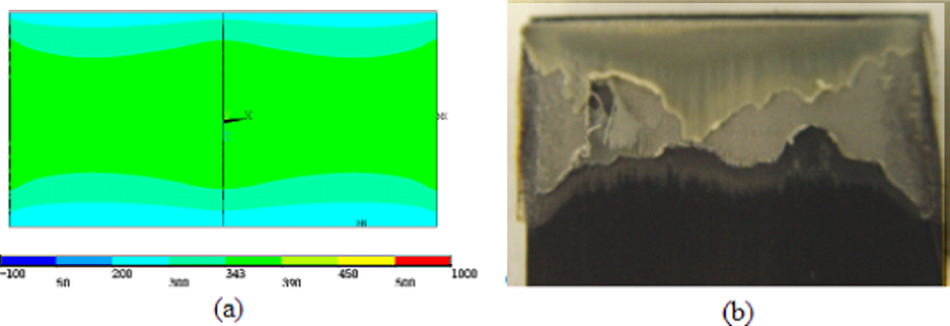
Weld interface of the samples welded at a processing temperature of 390°C using an optimum clamping distance of 0.8 mm. (a) Temperature contours and (b) fracture surface.

Figure 13.

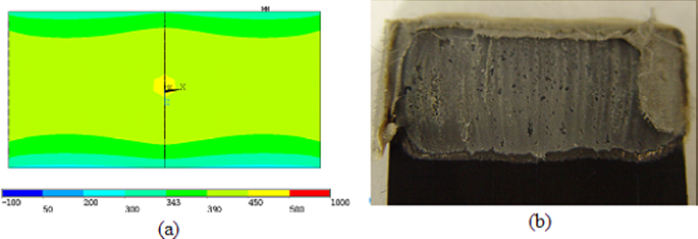
Weld interface of the samples welded at a processing temperature of 440°C using an optimum clamping distance of 0.8 mm. (a) Temperature contours and (b) fracture surface.

Table 4.

Lap shear strengths of joints welded using various processing temperatures and clamping distances.

Processing temperature (°C)	Clamping distance (mm)	Lap shear strength (MPa)
390	0.8	28.6
440	0	36.9
440	0.8	47.4
440	3.2	38.5

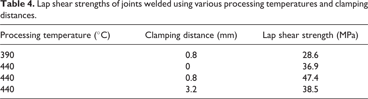
Figure 14 and 15 show the temperature contours and weld interface for the clamping distances of 0 mm and 3.2 mm, respectively. The results confirm that the clamping distance of 0 mm leads to unwelded edges, the clamping distance of 3.2 mm leads to overwelded edges and the optimum clamping distance of 0.8 mm (Figure 13) leads to a complete weld. Moreover, the optimum weld strength is obtained at the optimum clamping distance of 0.8 mm (Table 4).

Figure 14.

Weld interface of the samples welded at a processing temperature of 440°C using a clamping distance of 0 mm. (a) Temperature contours and (b) fracture surface.

Figure 15.

Weld interface of the samples welded at a processing temperature of 440°C using a clamping distance of 3.2 mm. (a) Temperature contours and (b) fracture surface.

Comparison between fracture surfaces and model prediction shows good qualitative agreement. However, measurement of the temperature profile during the welding operation would be needed in order to compare the results quantitatively. This will be done in future work.

Conclusions

Both 2D and 3D transient heat transfer finite element models were developed to simulate the resistance welding of APC-2/AS4 laminates. A single layer of stainless steel mesh sandwiched between PEEK polymer films was used as the heating element. The 2D model was used to investigate the influences of clamping distance and input power level on the local overheating (edge effect). The influence of the heat transfer along the length of the laminates was investigated using the 3D model. This work shows that:

1. The clamping distance has an influence on the local overheating at the edges of the welds. An optimum clamping distance can considerably enlarge the processing window. Optimization of the clamping distance is recommended to avoid polymer degradation at the edges of the weld.

2. High input power levels are not recommended, as they generally promote very narrow processing windows that may lead to polymer degradation at the edges of the welds.

3. The 3D model showed a large temperature gradient along the Z direction, due to thermal conductivity along the length of the laminates, which was not depicted in the 2D model. Hence, the 3D model should be used to study the heat transfer in resistance welding.

4. The 3D model qualitatively matches the experimental results.

5. Optimal lap shear weld strength of 47.4 MPa was obtained using the optimum combination of power level and clamping distance.

This work provides understanding of the effects of the resistance welding parameters such as clamping distance and power level on the thermal behavior of the welds, the temperature uniformity and, ultimately, the welds quality and strength. These conclusions are important to the aerospace industry, where thermoplastic composite structures are considered for the next generation of aircrafts.