Sage Journals: Discover world-class research

Abstract

French

The study of military spending has been an enduring concern within military sociology and political science. Methodologically, one of the biggest challenges lay in dealing with its heavy-tailed distribution influenced by the growing separation between China and the United States from the rest of the world. In the presence of outliers along the continuum of military expenditure, we should be paying more attention to portions of the distribution that don’t assume the values reported at the conditional mean. The article uses quantile regression modelling (QRM) to analyse the nuanced relationship between military expenditure and its predictors. It argues that classical linear regression produces average estimates that cannot predict values at different subsets of the data’s distribution, meanwhile QRM has relevant results in the search for noncentral values in the study of military expenditure often laying in the lower and the upper tails of the distribution.

Keywords

economic growth gross domestic product military expenditure quantile regression (QRM)statistical modelling

Introduction

Suppose military sociologists, political scientists or like-minded scholars were to study the wealth of information hidden in the relationship between military expenditure and socioeconomic growth in a large sample of countries, including advanced and emerging economies, with military spending and fiscal progress run at different speeds. The standard ordinary least squares (OLS) linear regression computes that the conditional mean of the outcome (military expenditure), given an independent variable (economic growth), may be expressed as the covariates’ linear function. Here we would treat cumulative military expenditure data with caution due to outliers and different types of error distribution. We know that the United States’ military expenditure is an outlier, that is, and extreme value compared to the bulk of the data. Classical regression might underestimate or overestimate the association of economic growth and military expenditure since we know this association will vary significantly along the continuum of military spending. The premise of standard regression wouldn’t consider that many important issues about military expenditure lie in modelling values at different subsets of the data’s distribution commonly referred to, in statistical parlance, as quantiles.

This article develops an argument for quantile regression modelling (QRM), a more flexible toolkit not operating in the restrictive fashion of conditional means. Introduced by Koenker and Basset (1978) in a seminal paper in the field of econometrics, QRM models conditional quantiles as functions of predictors enabling us to approach the relationships between variables while robust to outliers possibly perturbing the distributional mass (Koenker, 2017; Wang et al., 2018). QRM works as an extension of linear regression allowing new questions to be answered beyond looking at the mean average and describing the full conditional distribution of an outcome variable in terms of a set of predictors (Davino et al., 2014: ix).

What the article wants to do, essentially for an audience outside econometricians and other advanced analysts in quantitative sciences, is offer an overview without elaborate programming of quantile distribution and quantile regression modelling. It argues that QRM is a simple model to fit in statistical packages, easy to implement, and easy to interpret, being of interest to a more extensive, interdisciplinary range of authors. The article assesses the difference between observed values given the extreme variance in current military expenditure measures. To deal with potential shortcomings we might find when looking at military expenditure (or any other dependent variable if that was the case), the article uses a real dataset to test whether economic growth, measured in terms of gross domestic product (GDP) and gross national income (GNI), is associated with military expenditure. Examples will be presented using observations from 2001 and 2019 from the Stockholm International Peace Research Institute (SIPRI) military expenditure database. The article argues that looking at several quantiles simultaneously gives solid ground for further exploratory and hypothesis-generating research. As well, by looking at specific quantiles of interests, researchers can inspect and visualise hypotheses about countries falling more or less in predetermined subsets of data along the continuum of military expenditure. Scholars aware of the method can make an educated choice.

The article is organised as follows. First, it introduces and identifies a set of theoretical debates on military expenditure and economic growth. Second, it introduces the data and methodology. Third, it presents the results of descriptive quantile analysis and quantile regression models evaluating the association between military spending and economic size measures. Fourth, it discusses the implications of QRM and identifies some areas of advice for future users. The appendix provides the countries used in the exercises.

Thinking beyond averages

National authorities frequently take evidence-based decisions on outcomes that fall above or below averages of longitudinal data (Feinstein, 2015). Policy issues such as wages, educational tests scores, life expectancy, and military expenditure have continuous distributions that allow policymakers to infer ideas without incurring in overly technical calculations. The literature highlights a common “averages” debate around the globe, namely whether countries spend too much or too little on their military and defence budgets. O’Hanlon (2019) deems necessary a deeper examination on where the money is spent rather than at the average statistics which paint a disproportionate picture for U.S. military spending both nationally, that is, considering other domestic policy areas; and globally, that is in comparison to China and Russia, the second and third largest military spenders in the world. Similarly, Thorpe (2014) stresses the systematic study of the political economy of U.S. military spending and the interests behind the defence industrial complex instead of purely focussing on the expenditure levels sky-rocketing since World War II.

In the European Union, military expenditure is frequently debated among policymakers contemplating whether averages of expenditure meet the agreed 2 percent of GDP benchmark (Techau, 2015). ‘An average of 1.3 percent of GDP and great disparity over member states,’ concludes a briefing requested by the budgetary committee of the European Parliament discussing European security and strategic planning (Mathis, 2018). Observed values, as recorded in 2016, stretch from .3 percent of GDP in Ireland (the lowest), up to 2.4 percent in Estonia (the greatest). How realistic is the 2 percent average metric if countries have different fiscal necessities and allocate spending needs in ad hoc ways?

In China, where the increase for its 2020 defence budget is estimated at 6.6 percent average, the lowest year-by-year increment since 2016, the question is how to divide scarce resources between domestic social programmes and military modernization? In China economic growth has slowed down and the tension between spending priorities have increased (Glaser et al., 2020; Han et al., 2020). Regionally, Chinese military expenditure is also an outlier representing a particular security dilemma. The remaining East Asian states have dropped their defence spending averages to percentages of GDP similar to Latin America’s, mostly because they see little need to arm themselves in light of amicable coexistence and diplomatic solutions to escape conflict (Kang, 2017: 2).

Beyond the simplicity of reading averages, the continuum of military expenditure can spread out or get compressed in ways that are looking only at the mean won’t tell. Many researchers ‘increasingly want to know what’s happening to an entire distribution, to the relative winners and losers, as well as to averages’ (Das et al., 2019: 141). We know with certainty that greater or smaller spending trends usually have different effects on outcomes such as military modernisation, procurement, operational capabilities and industrial innovation (Bitzinger, 2011; Fiott, 2017; Solar, 2020; Zysk, 2021). In this case, the relationship of military expenditure, among other material indicators, and military effectiveness (Beckley, 2010) is often discussed and summarized in thoughtful ways but predominately focused on the countries in the upper tail of the expenditure distribution. What remains unanswered then is how do we unveil the nuanced distribution of military expenditure? This can be answered with the quantile model considered here.

Military expenditure and economic growth

A research theme that resurfaces from time to time among social scientists is the link between economic size and military spending, simply put, while the economy progresses and regresses, what happens to military expenditure? (Desli et al., 2017; Dunne and Smith, 2020; Emmanouilidis and Karpetis, 2020; Topcu and Aras, 2017; Yang et al., 2011). Recent studies highlight the different relationships between military spending and economic growth in developing and advanced economies. Clements et al. (2019) argue that countries with advanced economies and spending the most worldwide have remained avid in their expenditure since the 1970s. Conversely, in the developing economies military expenditure is constrained by social spending nowadays going towards the sustainable development agenda. For some of the top spenders, a strong and competitive military force is a way of signalling expected performance at war and obtaining concession without incurring physical conflict. Military power therefore carries a heavy economic burden as the state invest in costly military forces that don’t see much use (Slantchev, 2012). Elsewhere in the world, the ‘guns versus butter’ debate is more prominent as the prohibitive costs of military systems and the post-2008 austerity environment force leaders to rethink business strategies holding military budgets at bay while hoping to keep some competitive superiority (Rasmussen, 2015).

Economic progress has historically been monetized and measured by GDP growth, although it raises constant doubts among policymakers and scholars on the suitability of other accounting mechanisms giving weight to non-traditional economic products such as sustainability, well-being, and inclusive development (Coyle, 2015). Despite being a highly imperfect measurement, consistency and simplicity seem to be the logic behind using GDP as an aggregate measure of a country’s account of goods and services activity (Green and Herzberg, 2017).

The GDP’s continuum, however, is highly asymmetrically distributed in similar ways to global military expenditure. Nations with the biggest economies usually have the largest military spending (i.e., United States, China, Japan, Germany, France, Brazil, Italy, and India), and from this group the United States is by far the outlier accounting for one quarter of the global GDP measured in US$ trillions.

In order to maintain desired military capabilities and defence procurement levels, national leaders ought to be paying more attention to economic trajectories as an indicator of fiscal capacity to fulfil goals in the short and mid-term (Christie, 2017). Military expenditure and economic growth have a non-linear effect with economic growth, meaning that it changes in size and sign depending on the values of the variables used as predictors. For example, nations might increase their military expenditure in light of shocks to their security (Pieroni, 2009). In the words of Caverley (2018: 305) the ‘economics of producing war’ give evidence of some countries’ search for wealth primarily based on driving expenditure for greater military power. International threats and wars, imagined or real, inflate military costs despite the often overlooked diplomatic backchannels (Mueller, 2021).

Research expectations

What seems most important is the fact that the direction of the relationship is usually put to question, thus demanding more segmented analysis. For any given set of nations, can growth cause more military expenditure or can military expenditure be used to trigger growth? Can growth and military expenditure be pursued simultaneously thus having a bidirectional relationship? Using a sample of African countries, for example, Saba and Ngepha (2019) found that these relationships change among subgroups of nations, although when looking at the bulk of cases military expenditure has a significant negative impact on growth. In a similar fashion, Dunne and Tian (2015) argue that military spending has an adverse effect on economic growth using a panel of 106 countries over the period 1988–2010. Dividing the sample by levels of income, conflict experience, natural resources abundance, and openness and aid categories, they also concluded that military spending has a negative effect on growth.

The lack of consensus on the relationship between military expenditure on economic growth has motivated scholars more recently to seek additional confounders, such as investment channels or large security threats, although still not suggesting clear-cut relations between military expenditure and growth (Aizenman and Glick, 2006; Chan and Mintz, 1992; Dunne and Smith, 2020; Yang et al., 2011). This is unsurprising since there isn’t a cookbook solution to the development and deterrence paradox. Collier (2006) suggests that by reducing military expenditure, which in his view is not an effective deterrent of conflict, the freed resources could be better spent in growth initiatives that could gradually reduce risks and sources of conflict.

Why would some countries spend a considerable portion of their GDP on defence and the military while others do not? We know from previous studies that countless determinants such as external threats, form of government and congressional politics, electoral cycles, corporate profits, production capacity, or even geographical characteristics drive countries to increase military expenditure in favour of a perpetual state of mobilisation (Hewitt, 1992; Mintz and Ward, 1989; Nordhaus et al., 2012; Thorpe, 2014). To some observers, the general upward trend in defence spending is likely to continue as it is seen as a political priority among some of the most advanced Western economies (Béraud-Sudreau and Giegerich, 2018: 69–70).

On the other hand, we also know that the hot spots of conflict in the twenty-first century are not located in the global North, but rather in the global South where military expenditure is less documented. Thus, the fact that the most peaceful and wealthiest nations drive military expenditure to an extreme is not an accurate representation of what happens further down the curve of military spending. We tend to think that most countries need to afford a modern military and defence sector more or less irrespective of their financial situation, but clearly fewer states have the means to spend more on their capabilities and capacities in this day and age marked austerity (Donnelly et al., 2012). Moreover, we do not know if in this case the variables in question (economic growth and military expenditure) behave the same way if we were to analyse them in a large sample of highly diverse countries.

The article presents by way of example the effect of economic growth in military expenditures at two points in time in the last two decades. In theory, military expenditure data can involve dozens of good predictors. Only relative economic size is used here for illustration. The article argues that in order to empirically know more about the distribution of military expenditure and the effect of economic size we can employ quantile regression modelling. With many other datasets and research questions in mind, researchers will want to try out what effect can be found in selecting other predictors with less-known effects on the outcome of their choice.

Data and methodology

So far in the article I have orbited around data analysis concepts usually referred to as the measures of central tendency. These include the mean (the average of the data), the median (the middle value), and the mode (the value, or values, that occur the most). Conventional regression methods fit models using the conditional mean approach. Linear regression tells how the mean of the dependent variable changes for each unit change in the value of predictor variables (Li, 2015). As it happens when studying military expenditure, and across many other academic fields (i.e., management, ecology or health sciences, among others), we can be after an outcome that is heavily tailed and abnormally distributed, affected by outliers that increase or decrease the mean, finally influencing the results shown by the regression. Quantile regression is not a regression estimated on a quantile, or subsample of data. It uses all the sample and weights the distances between the values predicted by the regression line and the observed values, then minimises the weighted distances (Cook and Manning, 2013). The article thus challenges the idea that the outcome of interest in the explanatory variable is the same at all levels after adjustment for other explanatory variables (such as in ordinary least squares regression and logistic regression models). There are more groups of interests with differences across the distribution rather than only at the mean.

Take the case of Japan in the Asia Pacific and Oceania region. Although it sits among the top spenders in an area where spending has increased annually since 1989, Japanese military expenditure as a share of government allocation has fallen constant to a 2.5 percent since 2009 (SIPRI, 2020a). Military expenditure decreased and stagnated given the state reallocating resources to social and economic policy (Hughes, 2011). Still, Japan’s budget allocation, considering other factors affecting fiscal expenditure, give its military one of the highest budgets in the region (US$ 47.5 billion in 2019), also sitting at the high end of the global military expenditure continuum. The question that arises is how do we situate Japan, or any other country, within more appropriate parameters than the conditional mean of expenditure? By considering different levels of quantile distribution, we can set a path to explore how suitable covariates, of either social, economic or political nature, could have different effects on multiple countries while targeting the low, the median, and the high end of military expenditure.

The article aims to present a more concrete empirical explanation. The article draws on data from the SIPRI military expenditure database. Military expenditure was recorded in current dollars, according to calendar year and based on open sources. SIPRI gathers its data from national governments, international statistics, and specialist journals and newspapers. The eligibility criteria for time comparison includes countries with expenditure data in 2001 and 2019. Since the 9/11 terror attacks, military predominance has created a geopolitical environment where the state’s self-defence via militarisation is primordial (Byers, 2006). More recently, however, support for government spending on defence and national military purposes has begun to decrease considerably. A national survey in the United States revealed that 31 percent of people thought authorities spent too much on military expenditure, and 17 percent said they spent too little, compared to 19 percent and 41, percent respectively, in 2001 (Gallup, 2021). To Mann (2018) some societies, especially in the North, see the world through more peaceful eyes when their states need more resources to conduct a new kind of war, one that is distant, less visible and less central to their day-to-day lives. This thought is misleading as even if conflict happens more extensively, another thought Mann would disprove, the advanced economies usually are equally or more involved via technological and long-distance physical and digital weaponry.

Military expenditure is defined based on all current and capital expenditure on the armed forces, including peacekeeping forces; defence ministries and other government agencies; paramilitary forces; and military space activities. The data include expenditure on personnel; operations and maintenance; procurement; military research and development; military infrastructure spending, including military bases; and military aid (SIPRI, 2020b). Although it falls out of the scope of this article to present alternative sources of military expenditure, the advantages and limitations of SIPRI’s dataset is discussed by Smith (2017) who aptly addresses issues of reliability, validity, and comparability in the data-generating process. Brauer (2007), on the other hand, argued military budget data and economic growth measures should be treated carefully as they tend to be highly unstable across time.

For the purpose of using explanatory numerical variables, a GDP measure was included for the countries in the sample. Data are taken from the World Bank and OECD national accounts data files and are expressed in current dollars (World Bank, 2020). Also, a GNI measure was also considered from the same source (the World Bank uses Atlas conversion factor), this only for the year 2019 due to availability. Using the GNI indicator, the article defines three income categories: high (GNI per capita equal or above to US$ 12,536 per capita), medium (between US$ 12,535 and US$1,036), and low (US$ 1,035 or less). Appendix Table 1 presents the countries falling under each category.

The analysis includes descriptive statistics and regression models to assess empirical quantiles differences in 2019 compared to 2001. Models are fitted to compare classical linear regression and quantile regression estimates for each covariate in each year, and finally, sets of graphic coefficients are presented with their confidence intervals.

Fitting quantile regression to military expenditure

In a first step to introduce QRM, I illustrate the descriptive statistics of the quantitative response variable and the continuous predictor variables. It is worth noting at this point that quantile regression can also include more complex and advanced modelling with ordinal and categorical predictor variables as aptly explained by Davino et al. (2014). The authors also go through all the details to complete a QRM and data analysis in SAS, STATA and R packages which I do not present here.¹ Table 1 summarises military expenditure and income variables in 2001 and 2019. The mean and the highest values for the military expenditure variable have gone up considerably, from US$ 5.18 billion to US$ 13.17 billion, and US$320 billion to US$731 billion, respectively. A noticeable change is that the lowest value of the sample in 2019 is lower than in 2001. Regarding GDP values in US$ billion, the mean of the sample has also increased, as expected, from US$ 217 billion to US$ 567 billion, with the lowest and highest value also increasing in 2019 compared to 2001. Measures for GDP per capita have also gone up, and the GNI estimator shows similar values for 2019. Skewness measures show the degree and direction of asymmetry. We would expect symmetric distribution such as a normal distribution with a skewness value of zero, and a distribution that is skewed to the right has positive skewness. For both years measured, we can see skewness levels increasing from a low 1.8 for GNI in 2019, to a high 10.7 score of military expenditure in 2001. Kurtosis measures, on the other hand, show heavy tailed distributions. As a rule of thumb, light tailed distributions will have kurtosis less than 3.

Table 1.

Descriptive statistics

	2001							2019
	Obs.	Mean	SD	Min	Max	Skewness	Kurtosis	Obs.	Mean	SD	Min	Max	Skewness	Kurtosis
Military exp^*	141	5.18	27.55	.0003	320	10.7	122.8	141	13.17	65.96	.0001	731	9.65	102.7
GDP^*	151	217.27	954.33	.370	10252	8.64	86.0	149	567	2191.80	1.33	21433	7.63	66.6
GDP per capita	151	6318	9849	121	48179	2.03	6.5	149	14366	19982	261	114705	2.16	8.1
GNI	-	-	-	-	-	-	-	147	14209	19046	280	85500	1.80	5.53

Note: ^* expressed in US$ billions.

Source: Sipri (2020) and World Bank (2020).

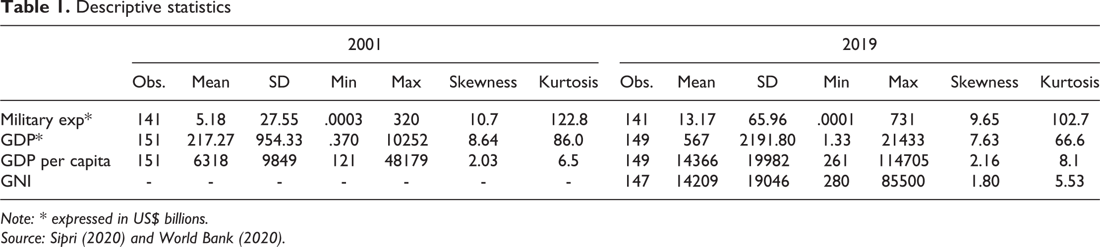
From Table 1, we do not have enough evidence to assume how military expenditure is distributed across countries in the sample. Figure 1 provides more evidence by making quantile plots of the raw data and the logged military expenditure variable for each year. The raw-scale military expenditure data is asymmetrical and with a heavy tail distribution. If it showed a normal distribution and direction of symmetry, and light tailed distribution, all the data would be plotted along the diagonal reference line. The plots show that the raw-scale variable is skewed right. A way to solve the high measure of skewness and extreme kurtosis is to use the natural log transformation of the military expenditure variable as shown in the lower two plots. Still, the actual values of the quantiles, or their equivalence in percentiles, can be subject to closer exploration.

Figure 1.

Distributional diagnostic plots for raw-scale and logged military expenditure in 2001 and 2019.

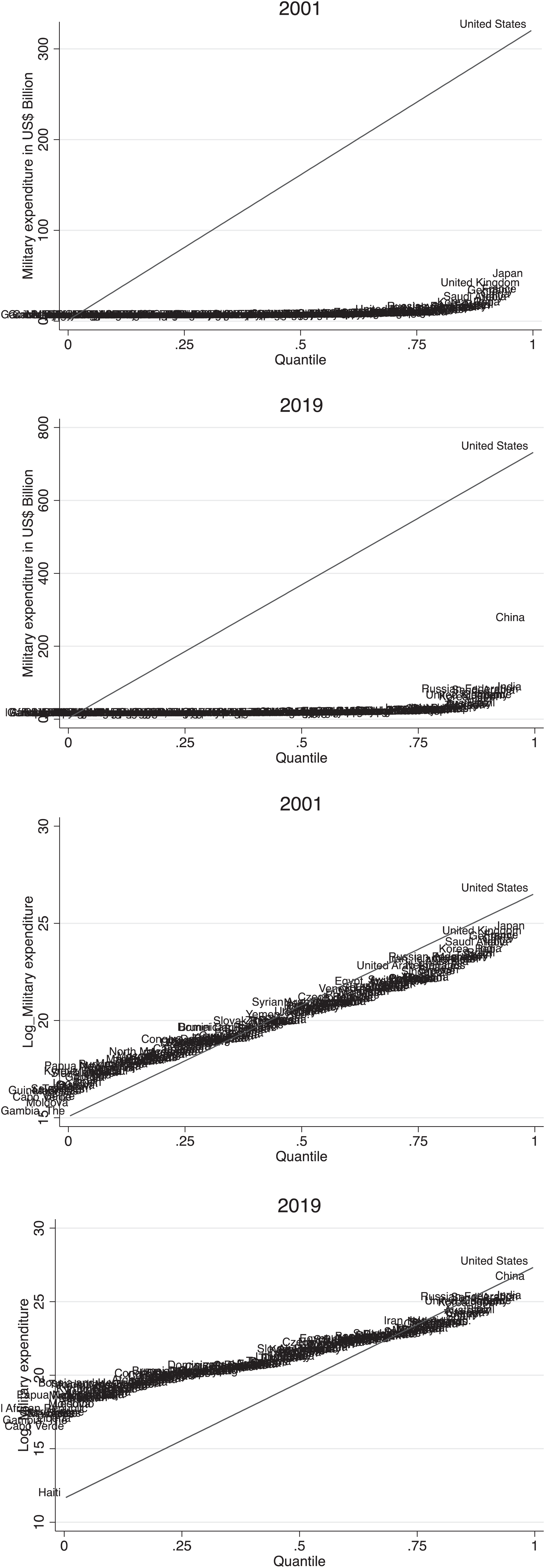
Table 2 presents the distribution of military expenditure in 2001 and 2019. Quantiles can be expressed as quartiles, quintiles, deciles, and percentiles. These are all valid ways of dividing the total number of rank-ordered cases or observations. Quantiles indicate the proportion of scores located below (and above) a given value (Vogt, 2011). For this part of the article, it is best to look at the untransformed data because we do not read percentiles using log-scale values. The analysis by columns shows that all the percentile increased in the most recent measure. The 50th percentile, also known as the median, increased from .34 to 1.00, that is, in 2019, half of the countries spent below US$ 1 billion, and half did above. Still, countries in the third quartile and above spent considerably more than the other two quartiles (as mentioned, from the plots in Figure 1 we know that the data has extreme outliers).

Table 2.

Military expenditure distribution by groups in 2001 and 2019

	Percentile
	1%	5%	10%	25%	50%	75%	90%	95%	99%
2001	.005	.010	.021	.055	.34	2.20	9.03	19.87	45.50
2019	.009	.025	.068	.23	1	5.17	20.46	48.65	261.08

Note: Military expenditure measured in US$ billion.

Source: Sipri (2020) and World Bank (2020).

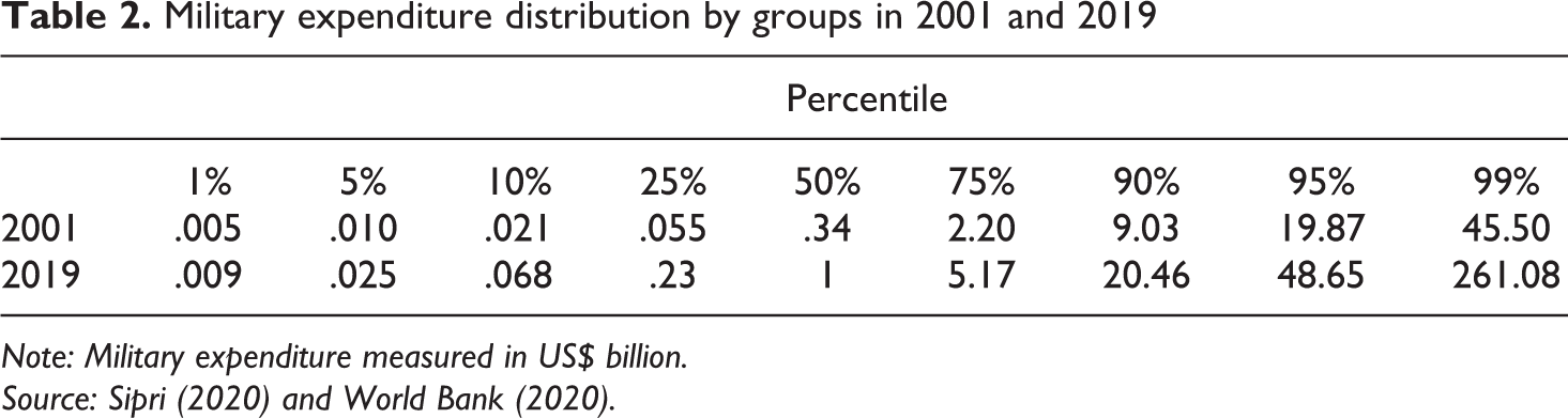
Figure 2 is a standard plot type showing level, spread, symmetry, and outliers with the numerical outcome scale on the y-axis, and the x-axis is categorical. The vertical box plots show the comparison of logged military expenditure for the groups observed in world regions for each pair of observations in 2001 and 2019. The boxes show a higher median (the line subdividing the boxes), and higher lower and upper quartiles for the logged military expenditure variable across all regions in 2019 in contrast to 2001. Whiskers extend to the outermost data points, and beyond lie individual data points at more than 1.5 times the interquartile range from the nearer quartile. Plots showing median and quartiles summaries provide more robust statistics than the mean and the standard deviation which can be highly sensitive to outliers (Cox, 2019).

Figure 2.

Box plots for logged military expenditure in 2001 and 2019 over regions, where 1 = South Asia, 2 = Europe and Central Asia, 3 = Middle East and North Africa, 4 = East Asia and Pacific, 5 = Sub Saharan Africa, 6 = North America, Latin America and the Caribbean.

Military expenditure disproportion is also evidenced by using the GNI measure to divide the sample in high-, middle- and low-income countries. Table 3 presents military expenditure distribution in 2019 in percentiles across the three groups. We can see that expenditure varies significantly across income groups, that is, looking at the rows, and by percentile, that is, looking at the columns (see Appendix Figure 1 for the scatterplots of raw-scale and logged military expenditure and GNI in 2019).

Next, the article introduces a comparison between ordinary linear squares regression (OLS) and QRM. Quantile regression allows examining the relationship between predictors and the outcome of specific quantiles of interests, sometimes at the extremes of the distribution, or multiple quantiles simultaneously (Staffa et al., 2019). The difference between OLS and QRM is that the latter unveils the entire distribution of the outcome being modelled, meanwhile the results of linear regression are interpreted in the context of the mean. Researchers give a twofold use to QRM in order to first deal with skewed distributions and outliers (Hao and DQ Naiman, 2007), and second, provide an estimated model for the conditional median function, and the full range of other conditional quantile functions; thus, ‘providing a much more complete statistical analysis of the stochastic relationships among random variables’ (Koenker and Xiao, 2002).

Table 3.

Military expenditure distribution by GNI groups: high, middle, and low-income countries in 2019

	Percentile
	1%	5%	10%	25%	50%	75%	90%	95%	99%
High (N=46)	.022	.083	.402	1.09	4.68	17.82	48.65	50.11	731.75
Middle (N=73)	.0001	.044	.08	.25	.62	3.46	10.08	27	261
Low (N=20)	0.14	.015	.021	.066	.17	.355	.595	.684	.722

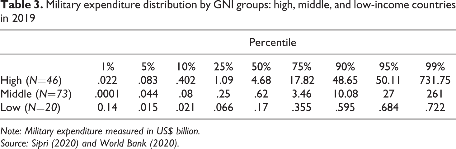
Note: Military expenditure measured in US$ billion.

Source: Sipri (2020) and World Bank (2020).

Suppose were to focus on the mean regarding the effect of economic growth on military expenditure. In that case, we could address the question ‘is economic growth important to understand the variation in military expenditure? However, we are after more intricate questions like ‘does economic growth have a significant effect on the tail levels of military expenditure?’ or ‘is the effect of economic growth as important on the tail levels of military levels as on its central level?’ Using QRM we can know the effect of the predictor at a specific quantile level of our dependent variable (Noh et al., 2013).

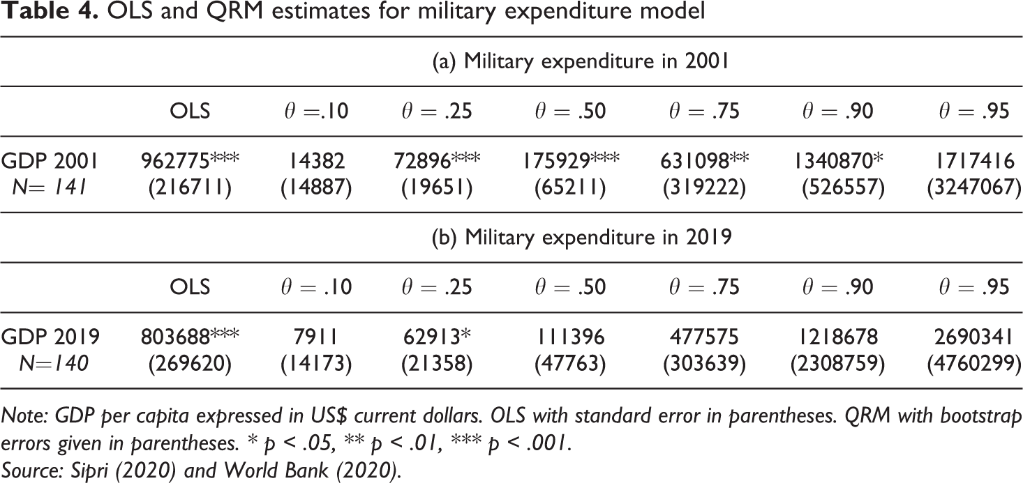
Table 4 presents the OLS coefficients, standard error, and an overall p value for the covariate. The quantile regression gives a coefficient estimate, bootstrap standard error, and p value for each model covariate at each quantile. Quantile regression coefficients describe how the associated quantile is affected by a 1-unit change in the corresponding factor. As argued by Staffa, Kohane, and Zurakowski (2019) quantile regression estimates for extreme quantiles, such as the 1st, 5th, 95th, or 99th quantiles, have more statistical uncertainty than central quantiles such as the median. Table 4 only uses one predictor (GDP per capita), but similar to a multiple variable linear regression, QRM can be used to specify coefficients on more than one covariate on a given quantile. Researchers are thus capable of introducing potential confounders for multivariable analysis testing the presence of predictors affecting a conditional quantile or across multiple quantiles (Rodriguez and Yao, 2017; Wang et al., 2018).

In general, quantile regression produces a distinct set of parameter estimates and predictions for each quantile level. In Table 4, the coefficients of the quantile regression models (a) and (b) should be interpreted in the context of the five quantiles θ = [0.1, 0.25, 0.5, 0.75, 0.9]. Because we produce different sets of parameters estimates the predictions for the quantile levels can and cannot be statistically significant. For example, the estimates for GDP in 2001 were not significant at both ends of the expenditure continuum (e.g., the 10th quantile and the 90th quantile).

Table 4.

OLS and QRM estimates for military expenditure model

	(a) Military expenditure in 2001
	OLS	θ =.10	θ = .25	θ = .50	θ = .75	θ = .90	θ = .95
GDP 2001 N= 141	962775^*** (216711)	14382(14887)	72896^*** (19651)	175929^*** (65211)	631098^** (319222)	1340870^* (526557)	1717416(3247067)
	(b) Military expenditure in 2019
	OLS	θ = .10	θ = .25	θ = .50	θ = .75	θ = .90	θ = .95
GDP 2019 N=140	803688^*** (269620)	7911(14173)	62913^* (21358)	111396(47763)	477575(303639)	1218678(2308759)	2690341(4760299)

Note: GDP per capita expressed in US$ current dollars. OLS with standard error in parentheses. QRM with bootstrap errors given in parentheses. ∗ p < .05, ∗∗ p < .01, ∗∗∗ p < .001.

Source: Sipri (2020) and World Bank (2020).

The QRM shows the median-regression model (the 50th quantile), which is the conditional median, and not the conditional mean as the OLS will report. These are both considered good cases for comparison because they try to model the central location of a response-variable distribution (Hao and D Naiman, 2007). The coefficient for GDP in the conditional-median model (a) for 2001 is U$ 175,929, which is lower than the coefficient in the conditional-mean model (OLS). This suggests that while an increase of one unit of GDP gives rise to an average increase of US$ 962,775 in expenditure, the increase would not be as substantial for most of the population. Similarly, the coefficient for model (b) for 2019 in the conditional-median model is US$ 111,396, lower than the corresponding coefficient in the conditional-mean model (b). However, in model (b) using a measure of GDP in 2019, the QRM coefficients were only statistically significant at the 25th quantile.

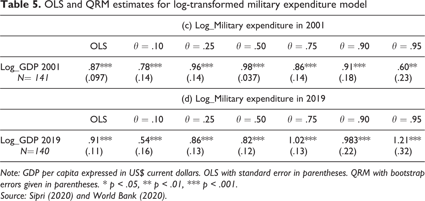
In Table 5, I return to the log-transformed data for military expenditure and GDP per capita in 2001 and 2019. The table presents the quantile regression to model for the five quantiles θ = [0.1, 0.25, 0.5, 0.75, 0.9]. I expect the quantile regression model on the median using a log-transformed response to be interpreted the same as when using non-logged data. That is, in the QRM models the conditional median model or 50th quantile, the regression line passes through data points dividing half the data points above the regression line and the other half falling below. Second, the QRM estimators for each quantile use the weighted data of the whole sample and not only the portion of the sample at that quantile (Li, 2015). The comparison of the OLS and QRM regression coefficients for models (c) and (d) reveal statistically significant estimates. In 2001 the conditional mean was lower than the conditional-median, and in 2019 the conditional mean was higher than the conditional-median. From the log-transformed models we see the benefits of using quantile regression as opposed to linear regression. By weighting different portions of the sample, the quantile regression coefficient estimates shown in models (c) and (d) allow us to detect differences in the upper and lower tails. Using model (d), for example, reveals a lower regression coefficient (β = .54, p < .001), meanwhile at the 95th quantile the coefficient is much higher (β = 1.21, p < .001). Also, looking at inter-quantile differences show that the 25th quantile regression coefficient is larger than the conditional-median estimate. As well, the 75th quantile coefficient is greater, only by a small difference, than the regression coefficient at the 90th quantile.

Table 5.

OLS and QRM estimates for log-transformed military expenditure model

	(c) Log_Military expenditure in 2001
	OLS	θ = .10	θ = .25	θ = .50	θ = .75	θ = .90	θ = .95
Log_GDP 2001 N= 141	.87^*** (.097)	.78^*** (.14)	.96^*** (.14)	.98^*** (.037)	.86^*** (.14)	.91^*** (.18)	.60^** (.23)
	(d) Log_Military expenditure in 2019
	OLS	θ = .10	θ = .25	θ = .50	θ = .75	θ = .90	θ = .95
Log_GDP 2019 N=140	.91^*** (.11)	.54^*** (.16)	.86^*** (.13)	.82^*** (.12)	1.02^*** (.13)	.983^*** (.22)	1.21^*** (.32)

Note: GDP per capita expressed in US$ current dollars. OLS with standard error in parentheses. QRM with bootstrap errors given in parentheses. ∗ p < .05, ∗∗ p < .01, ∗∗∗ p < .001.

Source: Sipri (2020) and World Bank (2020).

From Tables 4 and 5, we can suggest that QRM is a useful method, first, because it uses a general linear model on military expenditure to fit conditional quantiles without assuming a parametric shape in the distribution. Second, we can estimate the entire conditional distribution of the military expenditure while allowing the shape of the distribution to depend on the economic growth predictor. Third, the quantile plots reveal the effects of economic growth on different parts of the military expenditure distribution. And, finally, quantile regression can predict the quantile levels of observations while adjusting for the effects of covariates (Rodriguez and Yao, 2017).

Finally, I put the results of another quantile regression under graphical inspection. Figure 3 shows the slopes of the regression line across quantiles of the logged-transformed military expenditure scale and the three income categories of GNI. The conditional quantiles are shown in the x-axis and the coefficient values on the y-axis. The slope of the QR is represented in the green line and the black line is placed at the corresponding OLS estimates. For the low-income countries, the QR slope estimates are lower than the OLS counterpart below the 50th quantile, while the effect of the log-GNI on log-Military expenditure seems slightly higher at the 75th quantile. A similar reading can be done for the middle-income countries where the effect of the predictor over the outcome is stronger for the upper quantiles. For the high-income countries the QR slope estimates are higher than the OLS counterpart below the 25th quantile, while the effect of the log-GNI on log-Military expenditure seems slightly higher at the 90th quantile.

Figure 3.

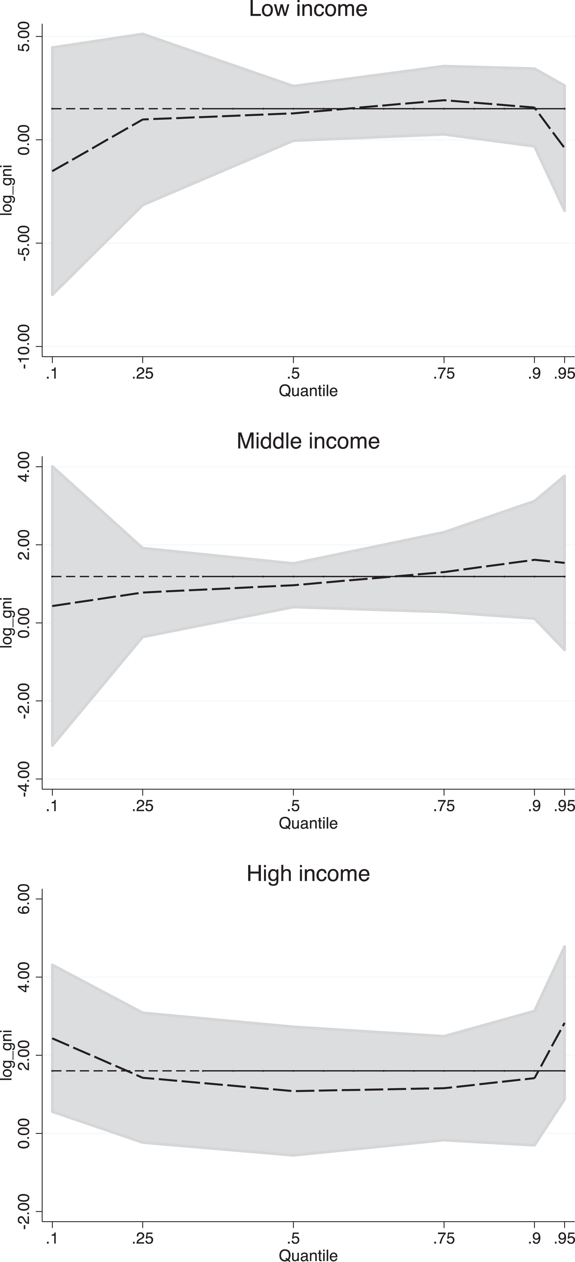
Graphical representation of the QRM estimates for log-transformed military expenditure model and GNI in 2019.

Limitations

The article has dealt with a central and straightforward methodological question dealing with heterogeneity and skewness in military expenditure and GDP data. The paper proposed QRM as a tool for panel heterogeneity, which is a problem not only for the study of data on government expenditure, but to many other themes based on sociological questions. A tool such as QRM is handy to consider in light of prevalent methodological problems any researcher will find when working with longitudinal and panel heterogeneity and skewness (Alejo et al., 2015; Lin and Wang, 2013; Rigby and Stasinopoulos, 2006; Scholtz, 2010).

To make the discussion clearer and pedagogical enough, a set of methodological suggestions from QRM should be transferable to other research projects. The use of QRM could indeed be directly related to projects beyond sociology, such as in the fields of economics, political economy, and even more broadly.² Although the purpose of this article was to test and illustrate QRM producing OLS estimates and comparing them to QRM estimates, it did not offer replication of previous studies. The paper began with a bivariate model to give support to the basic ideas that QRM is a stepping stone to replicate and complement multifaceted analyses on military expenditure such as those econometric models provided by Sandler and Hartley (1999), and more recently by Becker (2017), George and Sandler (2018), and Kim and Sandler (2020). Contrasting QRM to the use of rank correlations (common in the political economy literature), replicating analyses on the effects of military expenditure on GDP (Dunne and Smith, 2020), and then situating the results with larger meta-studies (Dunne and Tian, 2015) seems like doable and potentially natural next steps for quantile regression modelling. Recent examples of the disaggregation of defence expenditures, another way of dealing with heterogeneity, are provided by Bove and Cavatorta (2012), Becker and Malesky (2017), and Becker (2021). Replication of some of that work using QRM might also help make a better case for QRM as a tool to address heterogeneity and skewness issues with, for this case, military expenditure and GDP data.

Quantile regression’s methodological design, originality, and innovating approach have been used relatively little in, for example, the subfield of defence economics but as the article has shown it has been adopted theoretically and empirically. One way or another, previous works have utilized error correction when dealing with panel by including features like country fixed effects, panel-corrected standard errors, ARDL and error-correction models. Although the article compared QRM results to the most frequently used OLS estimates, the types of modelling mentioned above should also be put into comparison with quantile regression.

Conclusion

The theoretical and empirical data used in the article shed light on the complex relationship between military expenditure and economic progress in the rich economies and the rest of the world. The inequality in the distribution of military expenditure is similar to other topics for which social scientists have put their attention (i.e., wages, health access, drug and alcohol addictions, and life expectancy), and contribute with methodological innovation. Here I have argued the advantages of regression-modelling approaches in relation to the quality and nature of the data being explored. For the case of military expenditure data, which is non-normally distributed and have a non-linear relationship with predictor variables, the main advantage of using QRM is that it allows greater understanding of the relationships between variables outside of the mean of the data. On most occasion, we don’t want to know the estimates of regression methods in the “average” country. It is the countries with smaller and larger economies that present the most challenging questions in matters of military expenditure. What factors are important determinants of military expenditure for the small and large economies and what happens as we move along different subgroups of nations. While other scholars have suggested similar results could be estimated by stratifying different segments of the data and running separate regression, doing it in such a way would results in smaller sample sizes for each regression (Cook and Manning, 2013).

The article offered a gentle and systematic application to a methodology that can easily be adapted to more complex modelling. I provided solid arguments to use quantile regression in our search for non-central values in the study of military expenditure often laying in the lower and the upper tails. Quantile regression’s potentialities are undoubtedly beneficial to the study of military expenditure. In relation to its results, the linear regression estimated with raw-scale data obscured the effects and judged equivalent coefficients using only distributional moments such as the mean and standard deviation. The quantile function and the models using log transformation created a better model fit offering information on the whole conditional distribution of the response variable.

Footnotes

Acknowledgements

I wish to thank the editors at BMS and the two anonymous referees for their helpful comments during the review rounds.

Declaration of Conflicting Interests

The author declared no potential conflicts of interest with respect to the research, authorship, and/or publication of this article.

Funding

The author received no financial support for the research, authorship, and/or publication of this article.

Notes

Appendix

References

Aizenman

Glick

(2006) Military expenditure, threats, and growth. The Journal of International Trade & Economic Development 15(2): 129–155.

Alejo

Galvao

Montes-Rojas

, et al. (2015) Tests for normality in linear panel-data models. The Stata Journal 15(3): 822–832.

Becker

(2017) The correlates of transatlantic burden sharing: Revising the agenda for theoretical and policy analysis. Defense and Security Analysis 33(2): 131–157.

Becker

(2021) Rusty guns and buttery soldiers: Unemployment and the domestic origins of defense spending. European Political Science Review 13(3): 307–330.

Becker

Malesky

(2017) The continent or the ‘grand large’? Strategic culture and operational burden-sharing in NATO. International Studies Quarterly 61(1): 163–180.

Beckley

(2010) Economic development and military effectiveness. Journal of Strategic Studies 33(1): 43–79.

Béraud-Sudreau

Giegerich

(2018) NATO defence spending and European threat perceptions. Survival 60(4): 53–74.

Bitzinger

(2011) China’s defense technology and industrial base in a regional context: Arms manufacturing in Asia. Journal of Strategic Studies 34(3): 425–450.

Bove

Cavatorta

(2012) From conscription to volunteers: Budget shares in nato defence spending. Defence and Peace Economics 23(3): 273–288.

10.

Brauer

(2007) Data, models, coefficients: The case of United States military expenditure. Conflict Management and Peace Science 24(1): 55–64.

11.

Byers

(2006) Not yet havoc: Geopolitical change and the international rules on military force. In: Maiguashca

Armstrong

Farrell

(eds) Force and Legitimacy in World Politics. Cambridge: Cambridge University Press, 51–70.

12.

Caverley

(2018) The economics of war and peace. In: Gheciu

Wohlforth

(eds) The Oxford Handbook of International Security. Oxford: Oxford University Press, 304–318.

13.

Chan

Mintz

(1992) Defense, Welfare and Growth: Perspectives and Evidence. New York: Routledge.

14.

Christie

(2017) Does Russia have the fiscal capacity to achieve its military modernisation goals? RUSI Journal 162(5): 4–15.

15.

Clements

Gupta

Khamidova

(2019) Is military spending converging across countries? An examination of trends and key determinants. IMF Working Papers 19(196).

16.

Collier

(2006) War and military spending in developing countries and their consequences for development. The Economics of Peace and Security Journal 1(1): 10–13.

17.

Cook

Manning

(2013) Thinking beyond the mean: a practical guide for using quantile regression methods for health services research. Shanghai Archives of Psychiatry 25(1): 55–59.

18.

Cox

(2019) Stata tip 133: Box plots that show median and quartiles only. Stata Journal 19(4): 1009–1014.

19.

Coyle

(2015) GDP: A Brief but Affectionate History. Princeton: Princeton University Press.

20.

Das

Krzywinski

Altman

(2019) Quantile regression. Nature Methods 16(6): 451–452.

21.

Davino

Furno

Vistocco

(2014) Quantile Regression: Theory and Applications. Chichester: Wiley.

22.

Desli

Gkoulgkoutsika

Katrakilidis

(2017) Investigating the dynamic interaction between military spending and economic growth. Review of Development Economics 21(3): 511–526.

23.

Donnelly

Atkinson

Lindley-French

(2012) Affording war: The British case. In: Boyer

Lindley-French

(eds) The Oxford Handbook of War Edited. Oxford: Oxford University Press, 503–516.

24.

Dunne

Smith

(2020) Military expenditure, investment and growth. Defence and Peace Economics 31(6): 601–614.

25.

Dunne

Tian

(2015) Military expenditure, economic growth and heterogeneity. Defence and Peace Economics 26(1): 15–31.

26.

Emmanouilidis

Karpetis

(2020) The defense–growth nexus: A review of time series methods and empirical results. Defence and Peace Economics 31(1): 86–104.

27.

Feinstein

(2015) Misunderstanding data: Can researchers simplify longitudinal data for policymakers without it leading to errors? Available at: https://blogs.lse.ac.uk/impactofsocialsciences/2015/01/21/misunderstanding-data-feinstein/

28.

Fiott

(2017) A revolution too far? US defence innovation, Europe and NATO’s military-technological gap. Journal of Strategic Studies 40(3): 417–437.

29.

Gallup (2021) In-depth topics A to Z: Military and national defense. Available at: https://news.gallup.com/poll/1666/military-national-defense.aspx

30.

George

Sandler

(2018) Demand for military spending in NATO, 1968–2015: A spatial panel approach. European Journal of Political Economy 53: 222–236.

31.

Glaser

Funaiole

Hart

(2020) Breaking down China’s 2020 defense budget. Available at: https://www.csis.org/analysis/breaking-down-chinas-2020-defense-budget

32.

Green

Herzberg

(2017) Progress and regress: Understanding complex social measures and their trade-offs. Social Philosophy and Policy 34(2): 164–189.

33.

Han

Sadler

Quek

(2020) Guns and butter in China: How Chinese citizens respond to military spending. China Quarterly 245: 248–261.

34.

Hao

Naiman

(2007) Quantile Regression. Thousand Oaks: SAGE.

35.

Hewitt

(1992) Military expenditures worldwide: Determinants and trends, 1972–1988. Journal of Public Policy 12(2): 105–152.

36.

Hughes

(2011) The slow death of Japanese techno-nationalism? Emerging comparative lessons for China’s defense production. Journal of Strategic Studies 34(3): 451–479.

37.

Kang

(2017) American Grand Strategy and East Asian Security in the Twenty-First Century. Cambridge: Cambridge University Press.

38.

Kim

Sandler

(2020) NATO at 70: Pledges, free riding, and benefit-burden concordance. Defence and Peace Economics 31(4): 400–413.

39.

Koenker

(2017) Quantile regression: 40 years on. Annual Review of Economics 9: 155–176.

40.

Koenker

Bassett

(1978) Regression quantiles. Econometrica 46(1): 33.

41.

Koenker

Xiao

(2002) Inference on the quantile regression process. Econometrica 70(4): 1583–1612.

42.

(2015) Moving Beyond the linear regression model: Advantages of the quantile regression model. Journal of Management 41(1): 71–98.

43.

Lin

T-I

Wang

W-L

(2013) Multivariate skew-normal at linear mixed models for multi-outcome longitudinal data. Statistical Modelling 13(3). New Delhi: SAGE, 199–221.

44.

Mann

(2018) Have wars and violence declined? Theory and Society 47(1). Theory and Society 47(1): 37–60.

45.

Mathis

(2018) Defence: Member States’ Spending - European Parliament. Available at: https://www.europarl.europa.eu/RegData/etudes/BRIE/2018/621784/IPOL_BRI(2018)621784_EN.pdf.

46.

Mintz

Ward

(1989) The political economy of military spending in Israel. American Political Science Review 83(2): 521–533.

47.

Mueller

(2021) The Stupidity of War: American Foreign Policy and the Case for Complacency. Cambridge: Cambridge University Press.

48.

Noh

HGhouch A

Keilegom I

Van (2013) Quality of fit measures in the framework of quantile regression. Scandinavian Journal of Statistics 40(1): 105–118.

49.

Nordhaus

Oneal

Russett

(2012) The effects of the international security environment on national military expenditures: A multicountry study. International Organization 66(3): 491–513.

50.

O’Hanlon

(2019) Is US defense spending too high, too low, or just right? Available at: https://www.brookings.edu/policy2020/votervital/is-us-defense-spending-too-high-too-low-or-just-right/

51.

Pieroni

(2009) Military expenditure and economic growth. Defence and Peace Economics 20(4): 327–339.

52.

Rasmussen

(2015) The Military’s Business: Designing Military Power for the Future. Cambridge: Cambridge University Press.

53.

Rigby

Stasinopoulos

(2006) Using the box-cox t distribution in GAMLSS to model skewness and kurtosis. Statistical Modelling 6(3). SAGE Publications India: 209–229.

54.

Rodriguez

Yao

(2017) Five things you should know about quantile regression. Paper SAS525-2017: 2–6. Available at: https://support.sas.com/resources/papers/proceedings17/SAS0525-2017.pdf.

55.

Saba

Ngepah

(2019) Military expenditure and economic growth: evidence from a heterogeneous panel of African countries. Economic Research-Ekonomska Istraživanja 32(1): 3586–3606.

56.

Sandler

Hartley

(1999) The Political Economy of NATO. Cambridge University Press. Available at: https://econpapers.repec.org/RePEc:cup:cbooks:9780521638807.

57.

Scholtz

(2010) Inequality rose from above, so it shall fall again: Income skewness trends in 16 OECD countries as evidence for a second Kuznets cycle. International Journal of Comparative Sociology 51(4): 246–267.

58.

SIPRI (2020a) Global military expenditure sees largest annual increase in a decade – says SIPRI – reaching $1917 billion in 2019. Available at: https://www.sipri.org/media/press-release/2020/global-military-expenditure-sees-largest-annual-increase-decade-says-sipri-reaching-1917-billion.

59.

SIPRI (2020b) Military expenditure database. Available at: https://www.sipri.org/databases/milex

60.

Slantchev

(2012) Military Threats: The Costs of Coercion and the Price of Peace. Cambridge: Cambridge University Press.

61.

Smith

(2017) Military expenditure data: Theoretical and empirical considerations. Defence and Peace Economics 28(4): 422–428.

62.

Solar

(2020) China’s weapons transfer in the Western hemisphere. Journal of Strategic Studies 43(2): 217–244.

63.

Staffa

Kohane

Zurakowski

(2019) Quantile regression and its applications: A primer for anesthesiologists. Anesthesia and analgesia 128(4): 820–830.

64.

Techau

(2015) The politics of 2 percent: NATO and the security vacuum in Europe. Carnegie Europe (September): 1–30. Available at: https://carnegieendowment.org/files/CP_252_Techau_NATO_Final.pdf.

65.

Thorpe

(2014) The American Warfare State: The Domestic Politics of Military Spending. Chicago: University of Chicago Press.

66.

Topcu

Aras

(2017) Military expenditures and economic growth in Central and Eastern EU countries: Evidence from the post-Cold War era. European Review 25(3): 453–462.

67.

Vogt

(2011) Quantile. In: Dictionary of Statistics & Methodology. Thousand Oaks: SAGE, 256. Available at: https://dx.doi.org/10.4135/9781412983907.

68.

Wang

McKeague

Qian

(2018) Testing for marginal linear effects in quantile regression. Journal of the Royal Statistical Society. Series B: Statistical Methodology 80(2): 433–452.

69.

World Bank (2020) World Bank Open Data. Available at: https://data.worldbank.org.

70.

Yang

AJF

Trumbull

Yang

, et al. (2011) On the relationship between military expenditure, threat, and economic growth: A nonlinear approach. Defence and Peace Economics 22(4): 449–457.

71.

Zysk

(2021) Defence innovation and the 4th industrial revolution in Russia. Journal of Strategic Studies 44(4): 543–571.

Thinking beyond averages: Quantile regression modelling and military expenditure

Abstract

Keywords

Introduction

Thinking beyond averages

Military expenditure and economic growth

Research expectations

Data and methodology

Fitting quantile regression to military expenditure

Limitations

Conclusion

Footnotes

Acknowledgements

Declaration of Conflicting Interests

Funding

Notes

Appendix

References