
Abstract
In this article, we present an alternative approach to study dimensional stability and change in cultural divisions across time. Drawing on recent developments in Geometric Data Analysis (GDA), we combine the use of two distinct statistical techniques: Multiple Correspondence Analysis (MCA) and Class Specific MCA (CSA). Specifically, the approach allows for the systematic investigation of three key aspects: (i) whether and how the dimensionality and the structure of primary axes of geometrical spaces have been stable or subject to change; (ii) how the oppositions depicted by the axes of such spaces have become weaker or stronger; and (iii), how the connection between cultural divisions and class divisions has developed over time. Our exemplary case is Norway and the data stem from five different rounds of The Culture and Media Survey, conducted by Statistics Norway between 2000 and 2016.
Introduction 1
The question of stability versus change is fundamental in almost every sociological analysis. Methodologically, highly specialised statistical techniques, e.g. event history analysis or sequence analysis, have for instance addressed this problem by focusing on a restricted number of variables. Advanced techniques for dimension reduction, e.g. Geometric Data Analysis (GDA), has mainly been used on cross-sectional data to uncover structures at a specific point in time, leaving the question of cross-time stability or change a matter of speculation (though see Rosenlund, 2009). Thus, a methodology that in greater detail renders possible assessments of structural development across time is called for.
In this article, we aim to present a way of assessing temporal stability and change using GDA. Focusing on the question of whether and how the structure of cultural divisions has changed over time, as well as whether and how the homologous relationship between class divisions and cultural divisions has been subject to change, this article draws on the French statistician Brigitte Le Roux’s invention, Class-Specific MCA (CSA), to compare structural similarities and differences between geometrical spaces (Le Roux, 2014; see also Hjellbrekke 2018; Lebaron and Bonnet, 2019; Lebaron and Le Roux, 2015).
So far, this technique has mainly been used to analyse and compare structural correspondences between geometric spaces at one particular point in time (e.g. Bonnet et al., 2015; Hjellbrekke et al., 2015; Roose, 2015). In the analysis below, we will demonstrate how CSA also can be used to map the development of structural relations across time, and that the technique thus has a potential also for the analysis of structural stability and structural change. Inspired by Pierre Bourdieu’s classic study Distinction (1984), this will be done by way of an empirical study, aimed at mapping stability and change in cultural divisions across time, as well as stability and change in how such cultural divisions are connected to class structures.
We focus on the empirical case of Norway over a period of 16 years (2000–2016). Based on data from the quadrennial Culture and Media Survey (see e.g. Paulsen and Wilhelmsen, 2010), two sets of research questions are addressed: Has the structure of the Norwegian space of cultural practices and media preferences been stable or subject to change between 2000 and 2016? If so, are the dimensionality and the structure of the primary axes of the space similar or different? And have the oppositions depicted by these axes become stronger or weaker in this period? Has the connection between the space of cultural practices and media preferences and the class structure been stable or subject to change in this 16-year period? Has the strength of these connections changed over time? How do the class categories map onto the space of cultural practices and media preferences in the respective years? What are the distances between the categories?
Analysing structural homologies
In his now classic work Distinction (1984), Bourdieu set forth what has been labelled the ‘homology thesis’; that there exists a homology between the social space and the space of lifestyles. His claims were supported by analyses of French survey data from the 1960s and 1970s, demonstrating that the two spaces exhibited a similar structuring of their internal system of differences. The social space, i.e. Bourdieu’s model of the class structure, is primarily shaped by the distribution of, and relation between, economic and cultural capital (Bourdieu, 1984: 114–143). According to Bourdieu, the space of lifestyles, constructed on the basis of indicators of cultural practices and tastes in a wide range of cultural domains, exhibits a structure that is similar to that of the social space: ‘the spaces defined by preferences in food, clothing or cosmetics are organised according to the same fundamental structure, that of the social space’ (Bourdieu, 1984: 208). Bourdieu’s notion of homology thus pertains to the relationship between latent structures.
In this case, this means that the primary axes of the space of lifestyles map onto the primary axes of the social space in systematic ways. In order to prevent misunderstandings of the homology model, Bourdieu explicitly warned against what he called a ‘substantialist’ and ‘naively realist’ way of reading and assessing the validity of the model in other empirical cases, highlighting that one could not ‘reduce the homologies between systems of differences to direct, mechanical relationships between groups and properties’ (Bourdieu, 1984: 126). Instead, he argued, potential homologies can only by assessed by comparing ‘system to system’ (Bourdieu, 1998: 6). This implies that whatever is canonized, consecrated and recognized as markers of cultural distinction is context specific and may vary considerably across time and space. Yet homologies between social and symbolic structures may still be stable across contexts, as it does not pertain to connections between specific substances, e.g. between the upper class and a preference for works of classical music.
The ‘omnivore’ approach
Bourdieu’s work has been subject to multiple criticisms. The last 20 years, the proponents of the so-called omnivore-thesis has arguably been the most vocal. Within this framework, findings of broad and/or eclectic tastes among the upper classes are typically interpreted as a transformation of, and even challenge to, the old principles of cultural distinction (see e.g. Peterson and Kern, 1996). Many of these accounts are, however, not based on longitudinal analyses, but instead on the assumption that the upper classes used to be univores, exclusively enjoying highbrow culture.
Some notable exceptions have, however, sought to employ a longitudinal research design to investigate the rise and development of omnivorousness and also the transformations of cultural capital (e.g. DiMaggio and Mukhtar, 2004; Jæger and Katz-Gerro, 2010; Peterson and Kern, 1996; Rossman and Peterson, 2015; Katz-Gerro and Jæger, 2011). Jæger and Katz-Gerro (2010), for instance, attempt to track the development of omnivorousness by employing cross-sectional data collected at six points in time during a period of 40 years. Using a total of six indicators of cultural participation, categories are predefined as ‘highbrow’ (opera and classical music performances), ‘middlebrow’ (theatre and art museum/gallery attendance) and ‘popular’ (cinema attendance and reading newspapers). By way of latent class analysis, three clusters are identified: the ‘eclectic’ (a high probability of attending all six cultural activities); the ‘moderate’ (less likely to attend ‘highbrow’ activities compared to the ‘eclectics’); and the ‘limited’ (engaging only in ‘lowbrow’ activities) (Jæger and Katz-Gerro, 2010: 471-3). Focusing primarily on the ‘eclectic’ category, the authors compare the relative size of this cluster at six points in time, observing that cultural eclecticism has existed for the whole period and that it has slightly increased. This leads the authors to refute the homology model (2010: 479).
The analyses of Philippe Coulangeon (2011, 2021) lead to somewhat different conclusions. Although the general educational level has risen and institutionalized cultural capital thus has become accordingly less distinctive than what it was in the 1960s, and although the cultural oppositions in the 1960s now seem to have been replaced by an opposition between openness and closure towards cultural diversity, cultural class divisions have not become less prominent; they have rather been transformed. The dimension of openness versus closure to cultural diversity is not only structured along class lines. Cultural eclecticism is also a way of maintaining social distance: while the upper classes might exhibit increasing interest in select working-class cultural repertoires, Coulangeon argues, the working classes display ‘cultural insularity’ (Coulangeon, 2021: 358). Lifestyles and dispositions may have changed, but they are still classed, both in terms of their social structuring and in terms of their consequences in social life. Moreover, several authors have argued that the omnivore thesis is itself highly problematic in terms of its conceptual underpinnings, its operationalizations for empirical research, and the ways in which its proponents have interpreted empirical results (Brisson, 2019, 2021; Flemmen et al., 2018; Savage and Gayo, 2011) – a point also made by its originator, Richard A. Peterson (2005).
A relational approach
Bourdieu’s preferred approach has been developed further in the more recent methodological literature (Le Roux, 2014; Lebaron, 2009; Le Roux and Rouanet, 2010; Lebaron and Le Roux, 2015), and several studies have used various GDA techniques to assess the homology thesis. A space of lifestyles is typically constructed by subjecting a range of indicators of cultural taste to MCA. Subsequently, class categories derived either from various class schemes (see e.g. Bennett et al., 2009; Hjellbrekke et al., 2015; Le Roux et al., 2008), or from a separate MCA of a social space (see e.g. Flemmen et al., 2019; Prieur et al., 2008; Rosenlund, 2014), are projected into the space of lifestyles as supplementary variables. Structural correspondences are then assessed by investigating the pattering of how the class categories map onto the space of lifestyles, as well as calculating the distances between the categories.
Most of these studies have had to focus on analysing possible homologies at one given point in time. In some cases, it has been an alternative to use longitudinal data to construct separate spaces for a number of points in time, and then compare the structuring of the spaces. Alternatively, categories from other years might be projected into the reference space, in order to assess whether they have moved in one or more directions. Unfortunately, this juxtaposition of spaces does not allow for a direct investigation of how the dimensionality, the structure and the direction of the primary axes of the space have developed over time. Any inferences must be made between separately constructed spaces, rather from within the same space.
In the analysis below, we will demonstrate how this can be accomplished by way of CSA (Le Roux and Rouanet, 2010; see also Bonnet et al., 2015: 120–129; Le Roux, 2014: 264–269, 291–294). The active variables, i.e. the variables that are active in the construction the space of lifestyles, are those in the data from 2000. The active variables and their categories determine the axes orientation in this reference space. As in MCA, the contributions from the categories to the axes sum up to 100 for each axis for all active categories. Categories with contributions > the average contribution (1/K) should be emphasized in the interpretation of the axis (see Le Roux and Rouanet, 2010 for a detailed introduction to MCA).
Thereafter, the individuals from the subsequent years are projected into this space as supplementary individuals, or individuals that do not take part in the construction of the axes. We have chosen this option in order to study the stability or change occurring from a given point in time, in casu year 2000, instead of the deviation from the mean profile for the full period under investigation, which would have been the case if all individuals were defined as active. Thus, respondents from 2004 and later have neither a contribution to the inertia or variance in the global cloud, nor to any of the axes. But given that their positions in the space can be determined by their responses across the exact same set of variables as those of the active individuals (respondents in 2000), the supplementary individuals can also be projected onto the axes within the reference space, and thus be given factor coordinates in the same axes. This, in turn, opens up the possibility of doing a CSA on each of the subsets and to do a comparison of the results.
CSA can be compared to doing a non-normed Principle Component Analysis (PCA) on a subset of individuals, in which the individuals’ factorial coordinates one of the axes in the reference space are their values on the active variables. The geometrical distances between individuals are thus defined within a reference space constructed by means of MCA, and CSA then proceeds to establish new axes within a given subspace. Each subspace belongs to the same space as the global space generated by the original MCA. This also makes it possible to make direct statistical comparisons between this space and the sub-spaces, and to assess whether a given subgroup is structured in ways that are similar to, or different from the reference group and other subgroups. In our case, the reference group is constituted by the respondents in the survey from year 2000, and the subgroups the individuals in the surveys from the subsequent years.
The closer the distributions of the individuals in the subspaces are to the distributions of the individuals in the global space, the more similar the results from the CSA will also be to the results from the original MCA. In our case, this will be a clear indication of structural stability from t1 to t2. Conversely, the more the distributions in the subspaces differ from the ones in the reference space, the more the results from the CSA will differ from those obtained in the MCA, indicating structural change from t1 to t2.
The interpretation of the results from a CSA is done in the same way as when interpreting results from an MCA. The comparison between the CSA and the reference space proceeds in three steps: (i) comparing the eigenvalues from the MCA and the CSA; (ii) calculating the cosines for the angles between the axes from the MCA and the CSA; and (iii) comparing the contributions from the active categories to the retained axes between the subspaces.
Within social stratification research, CSA has been used to map for instance whether working class-internal differences in the French space of cultural consumption differs from the oppositions in the global space (Bonnet et al., 2015); whether the internal structuring of cultural consumption among particular age groups is similar to or different from other age groups (Hjellbrekke et al., 2015; Roose, 2015); whether there are homologies between the structures of various subfields within the field of power (Hjellbrekke and Korsnes, 2014); and whether the structuring of capital profiles among the women in the field of power differ from those of men (Hjellbrekke and Korsnes, 2016). Although it has not yet been used for the purpose of diachronic analysis, CSA is also well suited for investigating developments of spaces over time. Instead of running separate MCAs for each given point in time – and thus having to analyse each space in isolation from the reference space – CSA allows for a more direct measuring and comparison of how the structuring of the spaces have developed from a reference space.
And whereas Multiple Factor Analysis (Escofier and Pagès, 2016) makes it possible to also include metric variables in the construction of the space (e.g. the coordinates of axes from different spaces), CSA offers an interesting potential when mapping the development of structural homologies across time in sets of categorical variables. Instead of using cross-sectional data to map synchronic homologies between spaces, CSA permits using cross-sectional data, collected at different points in time, to map diachronic homologies in terms of similarities in the structuring of given space over a shorter or longer timespan. We will demonstrate this in an analysis of the Norwegian space of cultural participation and media practices over a period of 16 years.
Data and analytical strategy
The data stem from five different rounds of The Culture and Media Survey on cultural participation and media preferences, conducted by Statistics Norway (Bye, 2017; Høstmark and Lagerstrøm, 2007; Kleven, 2001; Paulsen and Wilhelmsen, 2010; Revold, 2013). The survey is distributed to statistically representative samples in the age span 9-79 years. Sample sizes vary from 2186 respondents in year 2000 to 1948 respondents in 2016. Net response rates have fallen from 70% and 69% in 2000 and 2004, to 57% and 59% in 2008 and 2012, and to 53% in 2016. But given the falling response rates for all surveys, the response rates are considered as acceptable. The overall data quality is also regarded as good. All data sets are available from the Norwegian Center for Research Data. The data were collected by way of personal interviews. We analyse a time period spanning a period of 16 years (2000-2016). 2 In our analysis, we focus on the adult population, and we have thus restricted the data sets to respondents aged 18–74. Respondents with a high number of ‘missing’ values have been excluded. The five data sets have been merged into one. We have included 28 of the variables on cultural and media practices that are identical across the original data sets. This allows for an analysis of both structural stability and change over the 16-year period under scrutiny.
The analysis is done in eight steps. First, subjecting the oldest data set (2000) to MCA, we construct and interpret the space of cultural participation and media practices. This serves as the reference space, or the baseline against which the results from the following years are compared. This construction is based on the respondents’ answers to all the 28 questions (see Matrix 1 below). Second, possible structuring factors (class, education, gender and age) are projected into the space as supplementary variables. The positions of the categories, as well as the distances between them, are then examined. In this way, one can assess the structural connections between the space of cultural participation and media practices and these structuring factors.
Third, the respondents in the 2004–2016 data sets are projected onto the space as supplementary individuals. These individuals have answered the exact same 28 questions, coded in the exact same way, as the reference individuals. As outlined above, the supplementary individuals have not been active in determining the orientation of the axes in the space, yet the individuals’ position in the space, as well as the distances between them, are determined by their scores on the active variables used to construct the space. Thus, they are situated within to the same space as the respondents in the 2000 data set.
Fourth, we use CSA to construct the subsequent subspaces for all the other measuring points (2004, 2008, 2012 and 2016), using the exact same active variables as in the baseline construction. In this way, instead of inferring distances between two or more points in two or more separate spaces, distances between categories’ positions can be compared directly within the same space. Fifth, we compare the eigenvalues from the MCA and the CSAs to see whether the oppositions depicted by the axes retained for inspection have become stronger or weaker during the 16-year period. Sixth, the cosines 3 for the angles between the axes from the MCA and the CSAs are compared to see whether the structuring of the spaces have changed over time. Seventh, the contributions from the active categories to the retained axes are compared, as part of the interpretation of the new axes from the CSAs. Finally, to assess how the structure of the spaces correspond to the class structure, 4 the class categories are projected into the reference space, and the categories positions on the axis inspected patterned along the relevant axes, as well as the scaled deviations between the categories (Le Roux and Rouanet, 2010). The same procedure is followed for each CSA subspace to assess whether the patterns and distances have changed over time.
To operationalize class, we have opted for the Oslo Register Data Class Scheme (ORDC) (Hansen et al., 2009; see Figure 1). This class scheme is inspired by Bourdieu’s model of the social space and distinguishes between classes and class fractions along two dimensions. It has a primary hierarchical dimension consisting of the total amount of capital and differentiates between four main classes: the upper, the upper-middle, the lower-middle and the working class. A second dimension of capital composition crosscuts these: the three highest classes are divided into cultural, economic and balanced fractions. ORDC is based mainly on occupational classification. Because of low frequencies for some class categories, we have used a five-class version of the scheme comprised by the following categories: cultural upper/middle class, balanced upper/middle class, economic upper/middle class, skilled/unskilled workers, and farmers/fishers/foresters.
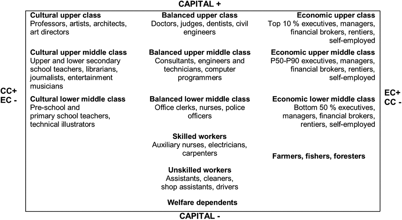
The ORDC class scheme
Educational capital is operationalized in two ways: first, in terms of whether the respondents have attained higher-education credentials (three categories: ‘no’, ‘yes’, some education from higher-education institutions’ and ‘yes, all education from higher-education institutions); and second, in terms of years of higher education (nine categories, ranging from 1–9 years). Age is coded into six categories: 18–24, 25–34, 35–44, 45–54, 55–64 and 65+. Gender is coded as ‘men’ and ‘women’.
Before we proceed to the analysis, it should be noted that there are some important limitations to our study. First, there is an element of political preconstruction in terms of the items included in the survey. The majority of the variables measure state-subsidized forms of culture. This means that the survey is skewed towards measuring participation in institutionally recognized culture, thus limiting the possibilities of mapping the social distribution of less legitimate cultural practices. It also means that what we refer to as ‘non-engagement’ should be seen relative to the legitimate items included in the survey and not as a ‘non-engaged’ lifestyle more generally. Second, some of the items included in the survey are broadly defined, meaning that the possibilities of analysing more fine-grained taste differences – for instance in terms of cultural hierarchies within cultural genres – is limited. Third, there are no indicators of lifestyle domains beyond cultural consumption and media preferences, meaning that we cannot construct an encompassing space of lifestyles, including for instance material consumption styles. This limits the possibilities of mapping intra-class divisions according to the capital-composition dimension of social space found in other Norwegian studies (Flemmen et al., 2019). There are good reasons to suspect that more substantial cultural changes would be detected if we had the proper data to go further back in time.
Even so, we still find the overall data quality to be strong. First, the response rates in these surveys are all above 50% (53% in 2016). Second, the included variables cover both classic ‘highbrow’ and ‘lowbrow’ indicators, and also a wide range of activities. They are thus valid indicators of broad spheres of cultural participation and of a wide range of media practices. Third, all included variables are present in all five data sets. Changes and stability can thus be mapped out with relatively great precision.
The reference space: The space of cultural participation and media practices in 2000
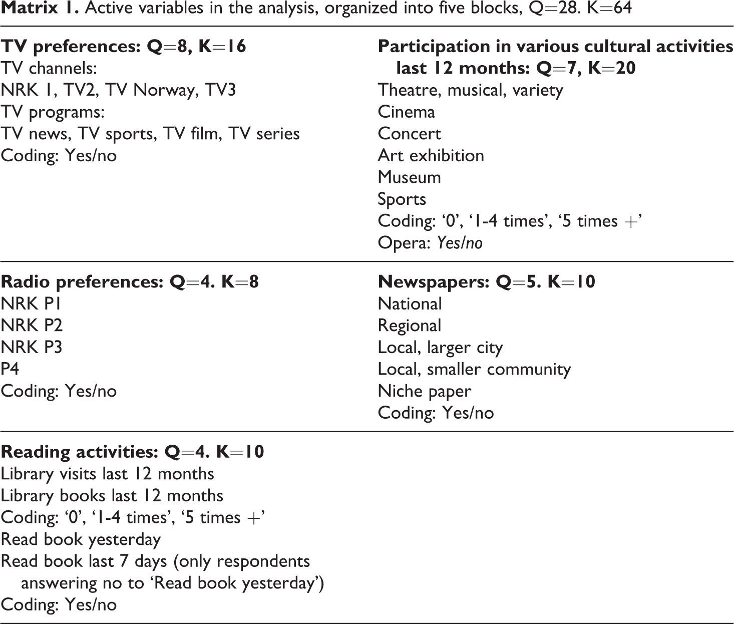
The reference space – the space to which all subsequent spaces are compared – is based on data from the 2000 survey. For the construction of this space, we have selected 28 variables, organised into five blocks. After recoding, there are 64 active categories.
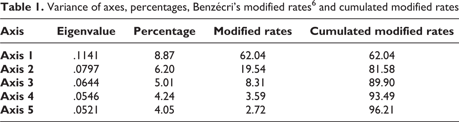
A standard MCA of these variables yields three axes for interpretation, summarizing 89.9 percent of the total variance in the cloud. As is clear in Table 1, Axis 1 is by far the most important dimension in the space, summarizing 62.04% of the total variance. Axes 2 and 3 summarise 19.54 and 8.31 percent, respectively. The relatively low variance summarised by Axis 3 means that this axis is clearly a second-order axis.
Variance of axes, percentages, Benzécri’s modified rates 5 and cumulated modified rates
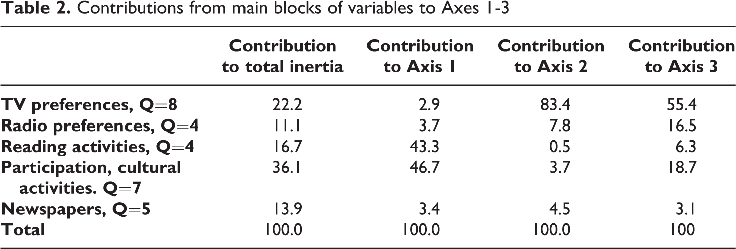
Although Axis 1 is by far the strongest dimension in the space, the results in Table 2 show that it does not represent a general opposition across all active variables. To simply the first, general interpretation, we have reorganized the variables into the same five block or headings as in Matrix 1, and summed up their contributions. Axis 1 first and foremost depicts an opposition related to two blocks of variables: participation in cultural activities and reading activities; 90 percent of the contributions to Axis 1 stem from these two blocks.
Contributions from main blocks of variables to Axes 1-3
Active variables in the analysis, organized into five blocks, Q=28. K=64
Axis 2, on the other hand, receives >95 percent of its contributions from the media blocks (TV preferences, radio preferences and newspapers). Axis 3 is slightly more balanced in terms of contributions from the various blocks. Yet it is clearly a media dimension: 75 percent of its contributions stem from the three media blocks.
Interpretation of Axis 1
Figure 2 depicts the categories with the highest contributions to Axis 1. The axis is dominated by categories involving legitimate and institutionally recognised cultural forms such as opera, art exhibitions, theatre, as well as reading and visits to the library. The only media category with a contribution above the threshold (>1/K. i.e. 1/64 = .0156) is NRK P2, a national public radio channel with the most distinct legitimate cultural profile in Norway. To the left of the figure, we find active engagement in all of these activities. To the right, we find the opposite: non-engagement in all these legitimate cultural forms. Axis 1 thus depicts an opposition between engagement and non-engagement in institutionally recognized forms of culture.
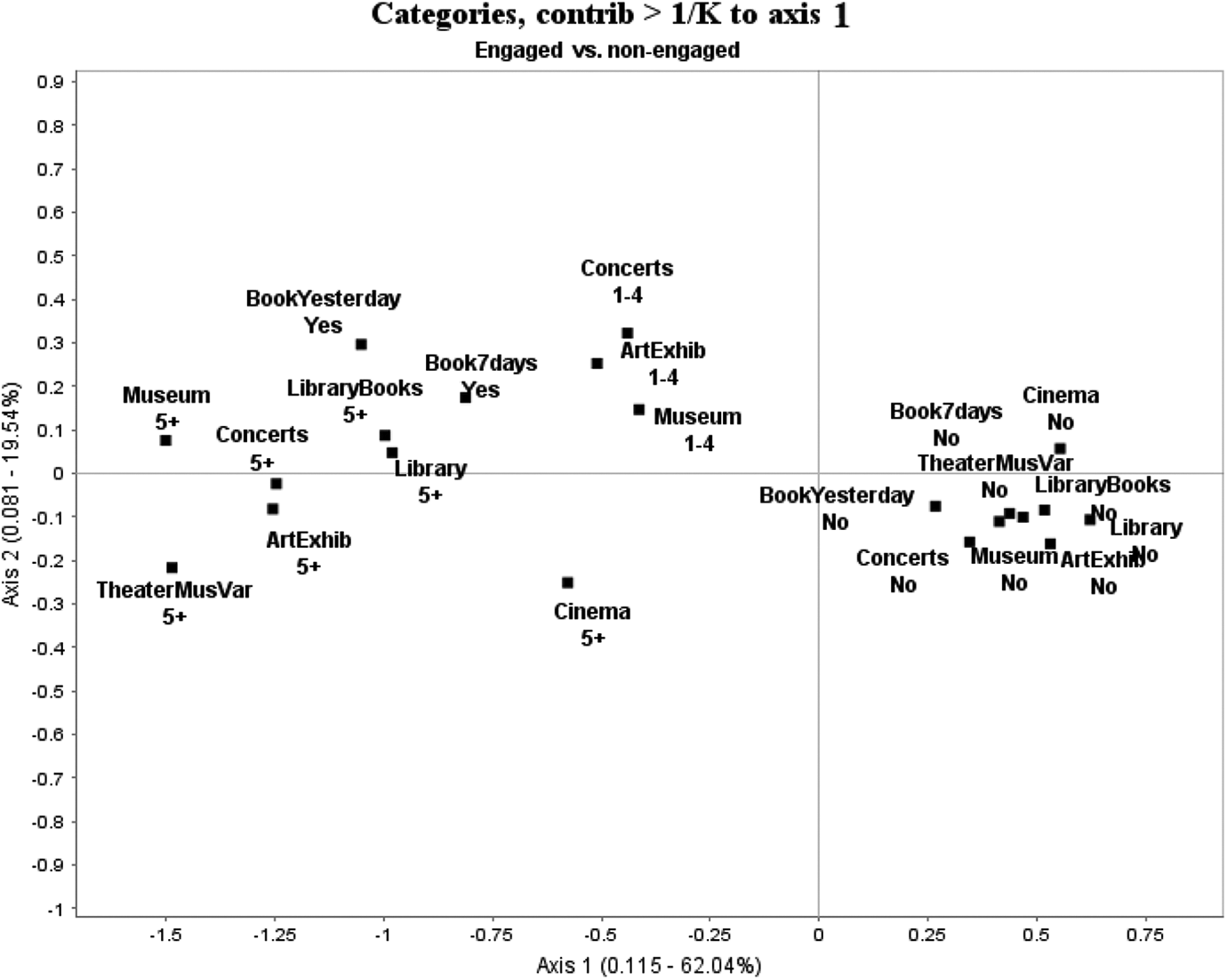
Categories with the highest contributions to Axis 1, factorial plane 1–2
Interpretation of Axis 2
Figure 3 depicts the categories with the most important contributions to Axis 2. This axis stands out as a strong media axis, dominated by categories involving television, radio and cinema. At the top of the figure, we find distinct non-engagement in media participation, in particular television. At the bottom of the figure, we find those who are highly engaged in cinema and various television channels and programmes. Axis 2 thus depicts an opposition between engagement and non-engagement in visual media.
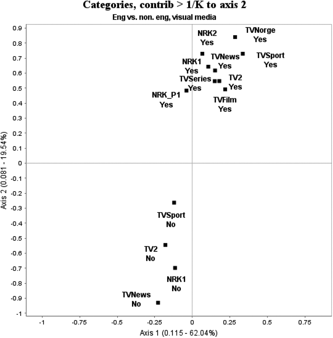
Categories with the highest contributions to Axis 2, factorial plane 1–2
Interpretation of Axis 3
Figure 4 depicts the categories with the highest contributions to Axis 3. The axis receives its highest contributions from a subset of media variables. At the top of the figure, we find several indicators of non-engagement in commercial media (the television channels TV Norway and TV3, and the radio channel P4) and media explicitly targeting young audiences (the radio channel NRK P3). This non-engagement is combined with engagement in cinema, reading library books, as well as established, national public media (television channel NRK1 and radio channel NRK P1). At the bottom of the figure, we find the opposite profile: non-engagement in established, national public media, combined with engagement in TV series and art exhibitions. In sum, the axis depicts an opposition between engagement and non-engagement in specific forms of media. Although not a clear-cut opposition in terms of the content of these media, the axis describes an opposition between commercial media preferences and state-funded media preferences.
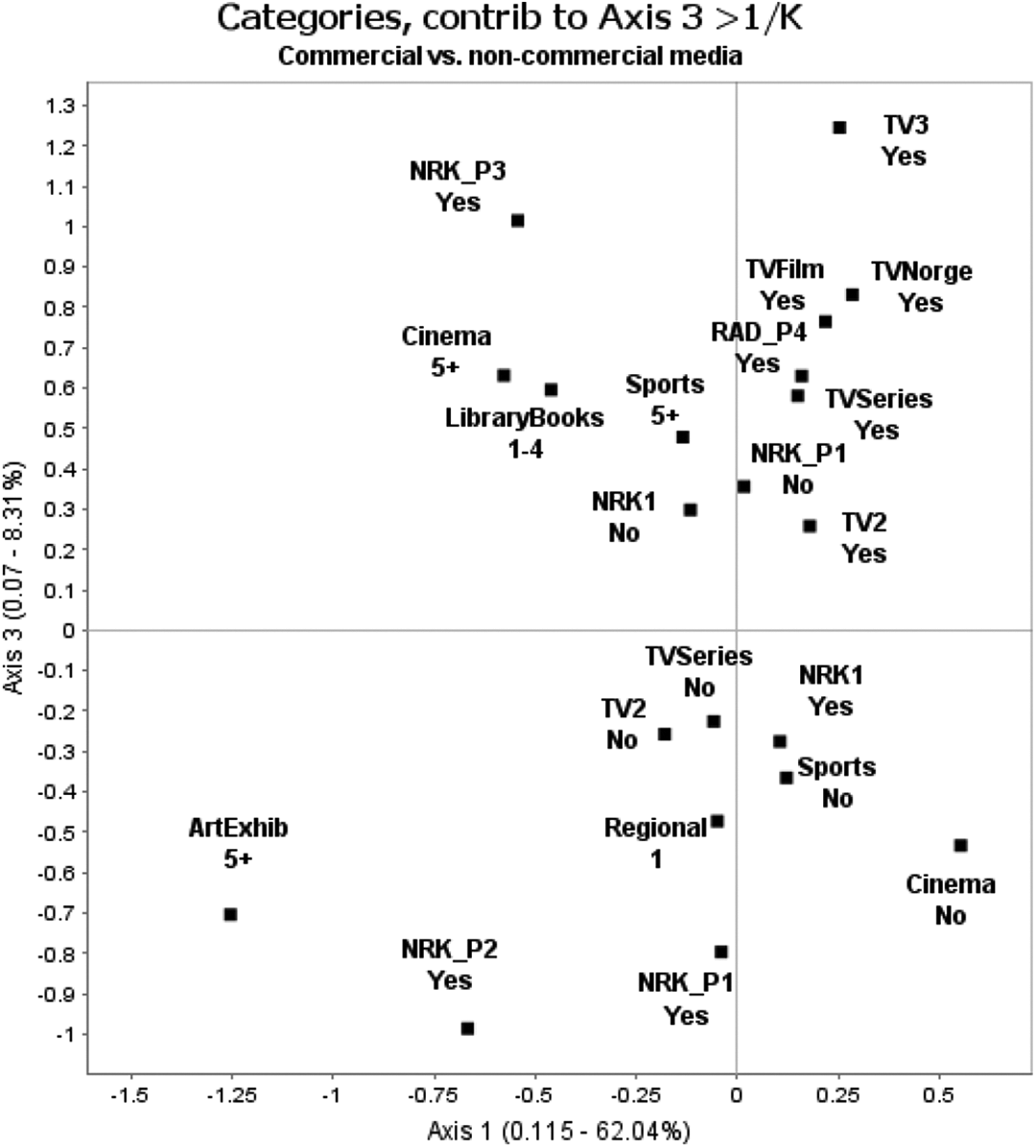
Categories with the highest contributions to Axis 3, factorial plane 1-3
Structuring factors
Figures 5 and 6 depict how class position and level of educational capital systematically correspond to Axis 1. Those with no higher-education degree and those in working class positions are drawn towards the ‘non-engaged’ pole; having attained a university degree is drawn towards the ‘engaged’ pole; while having attended some university courses is occupying a middle position. 6 The scaled deviation between the categories indicating no higher education and having completed a university degree is notable: >.80.
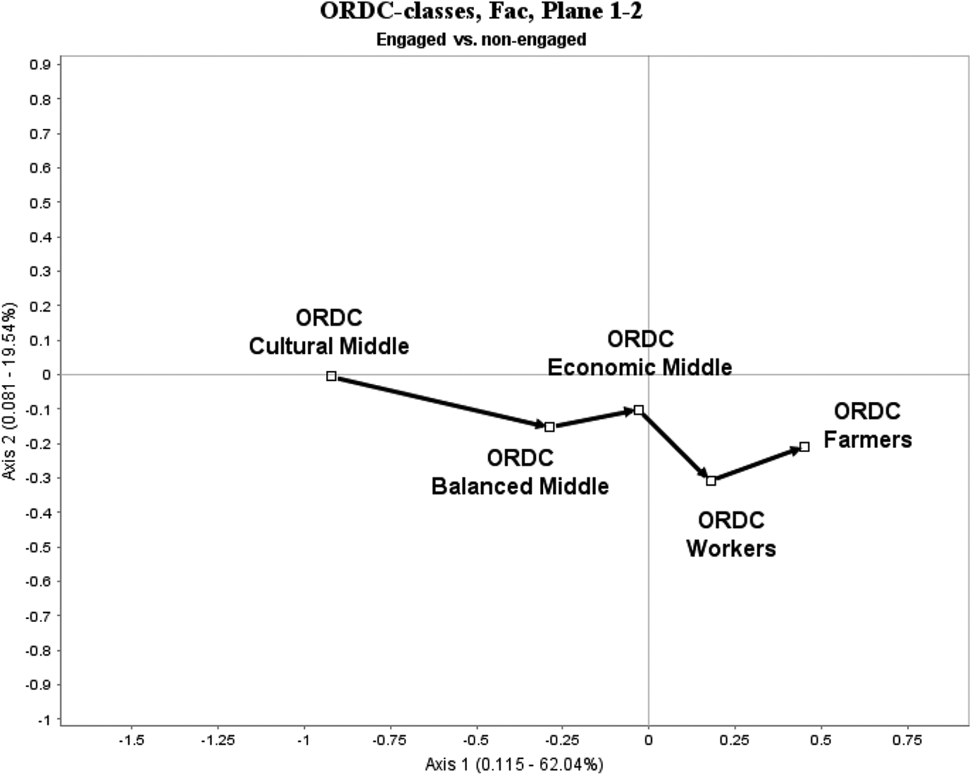
ORDC classes in factorial plane 1-2
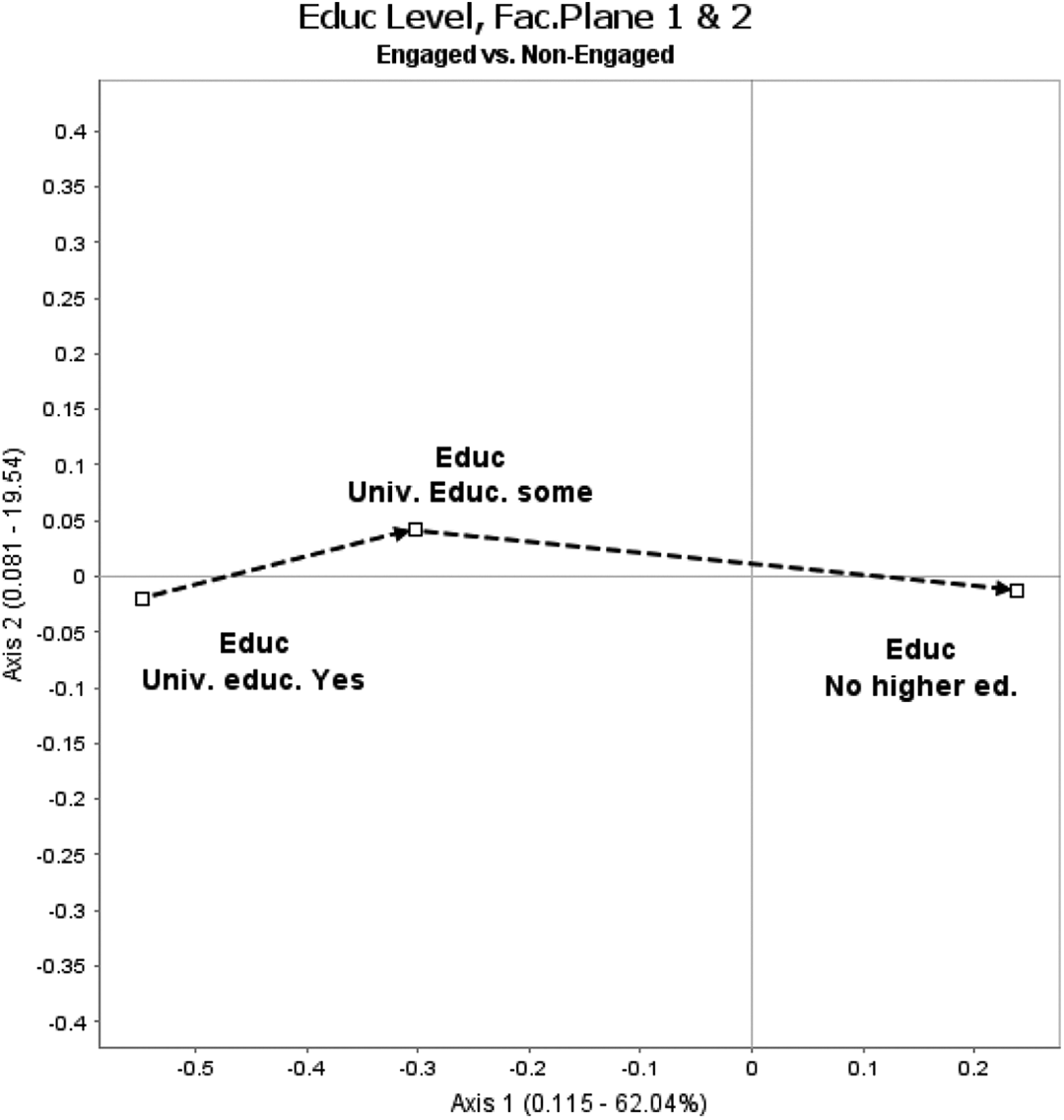
Education in factorial plane 1-2
Previous studies have revealed a strong association between age and cultural practices (see e.g. Bennett et al., 2009). The same association is found in this data set. Figure 7 displays factorial plane 1-3 in the space from 2000. Along Axis 3, the youngest respondents are drawn towards the commercial media pole, while the older respondents are drawn towards the state-funded media pole. The scaled deviation between the oldest and the youngest respondents is >1.5, i.e. a large deviation.
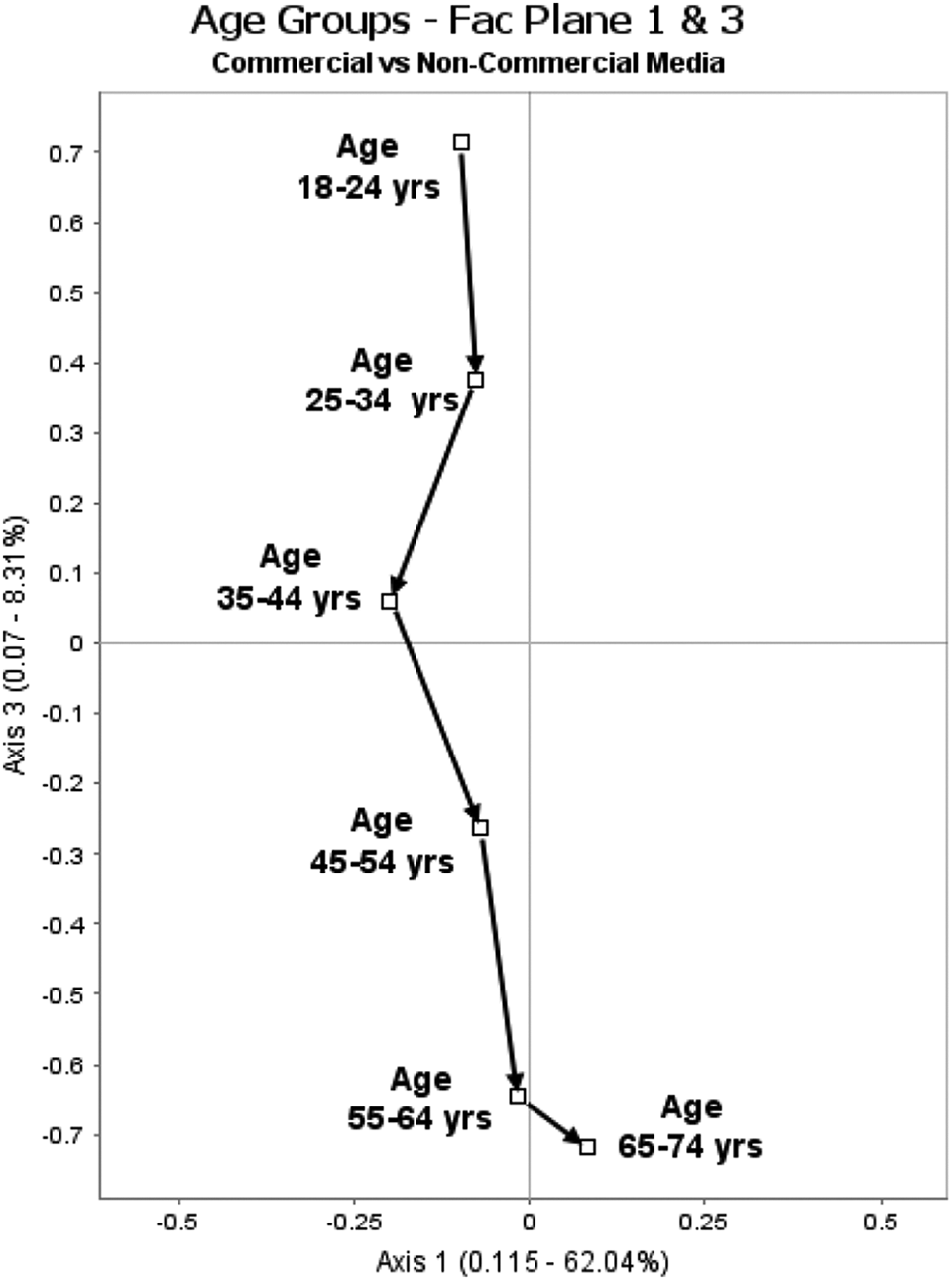
Age groups in factorial plane 1-3
Along Axis 2 (not shown), the younger respondents are drawn towards the pole signifying engagement in visual media, while the older respondents are drawn towards the pole signifying non-engagement. The scaled deviation between the youngest (18-24) and the oldest (64-74) respondents is notable, at .76, but not as clear as the deviation along Axis 3.
Somewhat surprisingly, gender differences (also not shown) are far less clear. Although more women than men are drawn towards the ‘legitimate’ pole, the scaled deviation is only .33 along Axis 1 (and <.03 on both Axes 2 and 3).
Stability and change, 2000-2016
Having mapped the structures of the reference space from 2000, we now proceed to the analysis of structural stability and change. The results of the CSAs of the data sets from 2004-2016 are summarized in Table 3. For all five axes included in the analysis, the eigenvalues are stronger in 2016 than in any of the previous years. This indicates that all the oppositions depicted in reference space have intensified over the 16-year period.
Eigenvalues, MCA of data from 2000. Specific eigenvalues from CSA of data from 2004–2016
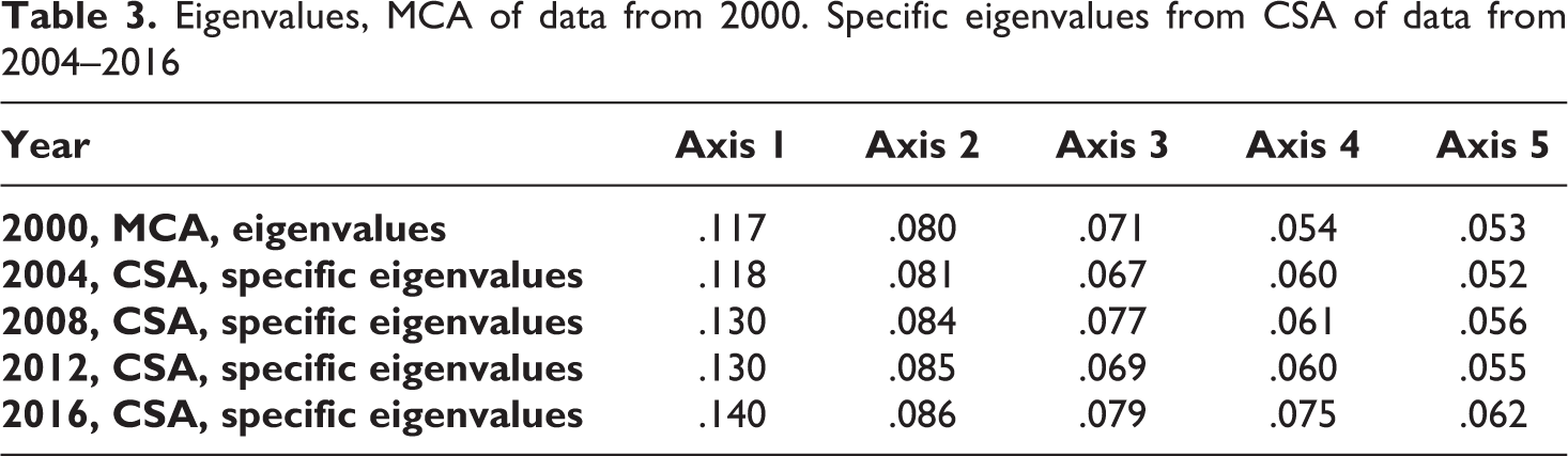
There are, however, some nuances to this general picture. First, the eigenvalues from the CSAs indicate that the oppositions along the first two axes are continuously getting stronger during this period. In other words, the difference between those who are engaged in legitimate culture and those who are not, as well as the difference between those who are engaged in visual media and those who are not, have intensified systematically between 2000 and 2016. Second, the trend, if any, for Axis 3 is less clear. While the eigenvalues for the first two axes steadily increase, the eigenvalues for Axis 3 shift in both directions. This might indicate an element of structural instability: the development of the opposition between commercial media preferences and state-funded media preferences does not seem to follow a specific pattern in this time period. Third, the eigenvalues for Axis 4 indicate a change from 2000 to 2004, followed by 8 years of structural stability. Notably, however, the eigenvalues increase sharply between 2012 and 2016, indicating that this opposition has gained importance at the end of the period.
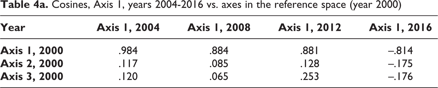
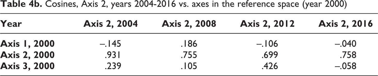
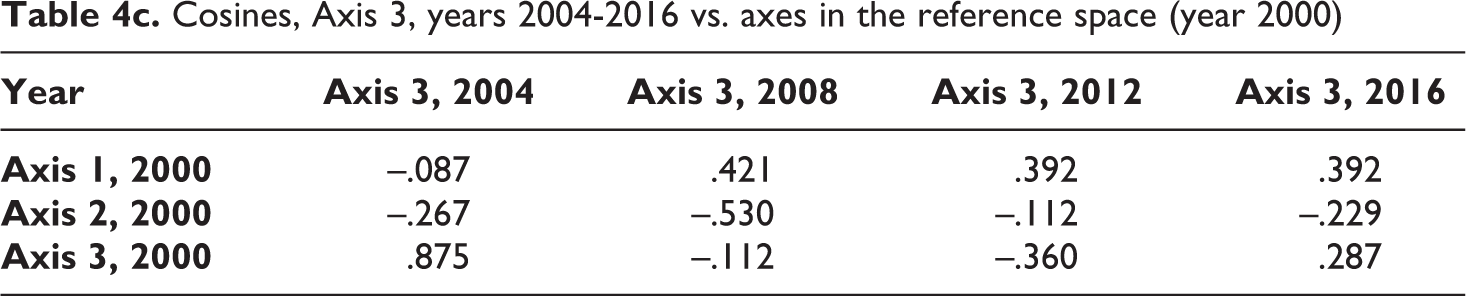
To assess developments in the structuring of the spaces, we measure the ways in which the primary axes of the CSA spaces deviate from the primary axes of the reference space. Tables 4a -c depict the cosine values (or correlations) between the axes of the reference space and the axes of the spaces for the four subsequent surveys.
Cosines, Axis 1, years 2004-2016 vs. axes in the reference space (year 2000)
Cosines, Axis 2, years 2004-2016 vs. axes in the reference space (year 2000)
Cosines, Axis 3, years 2004-2016 vs. axes in the reference space (year 2000)
In 2004, the cosine values for all the axes are high, meaning that the structuring of the space has not changed much since 2000. We have therefore decided not to go into detailed examination of the results from the analysis of the 2004 data.
From 2008 and onwards, however, the structuring of the space starts to change. Axis 1 is increasingly rotating away from the reference space. In 2016, the cosine value is -.81, which means that Axis 1 has rotated 36 degrees during the 16-year period. This is mainly due to a high contribution from one single category, ‘Going to live concerts 5 times or more per year’, a practice that plays a far more important role in the CSA than in the MCA. This is most likely caused by changes in the young practices (e.g. increased orientation towards the internet): in our data sets, this change makes going to live concerts 5 times or more per year more distinctive for this age group. We regard this as an artefact of the available variables for constructing the reference space. Apart from this, the list of the most contributing categories and variables remain more or less the same from year to year.
The changes for Axis 2 are more pronounced. In 2008, it has rotated 40 degrees from the original 2000 axis, and in 2012, it has rotated a full 45 degrees. Like Axis 1, this change in orientation stems mainly from a higher contribution from one category - ‘Going to live concerts 5 times or more per year’ (2008: 25 percent; 2012; 16 percent; 2016; 20.7 percent). Nonetheless, in all three data sets (2008. 2012 and 2016), the axis remains strongly related to media practices in ways we have outlined above, i.e. engagement versus non-engagement in traditional, visual media. In sum, the changes indicate that elements from Axes 2 and 3 in the reference space are integrated in the new Axis 2 in the subsequent CSAs.
For Axis 3, the changes are more profound. As the cosine values indicate , this axis takes on a new orientation vis-à-vis the reference space from 2008 and onwards. The correlation between the new axis 3 and the old axes 1-3 are all low, and the angle degrees between the new axes 3 and the old axis 3 are all >45 degrees. Axis 3 in the 2016-data has a cosine of .287 against axis 3 in the 2000-data, i.e. an angle between the two axes of 73.3 degrees. This might indicate axis instability and fluctuations in what oppositions the new Axis 3 describe. In the reference space, Axis 3 describes an opposition between commercial and state-funded media preferences. In the CSA based on the data from 2008, Axis 3 is strongly dominated by high contribution from the category indicating high frequenting of concerts (24 percent), watching the news on television (6.1 percent) and watching TV2 (5.2 percent) versus not watching the news on television (9.2 percent) and not watching the major TV channels (Not TV2: 5.1 percent; Not NRK 1: 4.6 percent).
In 2012 and 2016, this shifts to an opposition between high attendance at music concerts (a contribution of 31.3 percent in 2012 and 14.8 percent in 2016), listening to the youth radio channel, NRK P3 (2012: 5 percent; 2016: 18.8 percent;), on the one hand and, on the other, the most eager book readers. i.e. having read a book yesterday (2012: 9.3 percent; 2016: 5.8 percent) and having read a book the last 7 days (2012: 6.4%; 2016: 5.1%). Since the eigenvalues for axes 4 and 5 are low, these are not retained for a more detailed interpretation.
Social class: Stability and change
Above, we have seen how the structuring of the space of cultural participation and media practices has developed over time. We now turn to an assessment of whether the connection between this space and the class structure has been stable or subject to change. In Table 5 the coordinates for the ORDC classes on the first three axes of the CSAs from 2008, 2012 and 2016 are listed. The coordinates are retrieved from non-normed PCAs of the cloud of individuals. 7
Coordinates in cloud of individuals, ORDC-classes, MCA 2000, CSAs 2008, 2012 and 2016
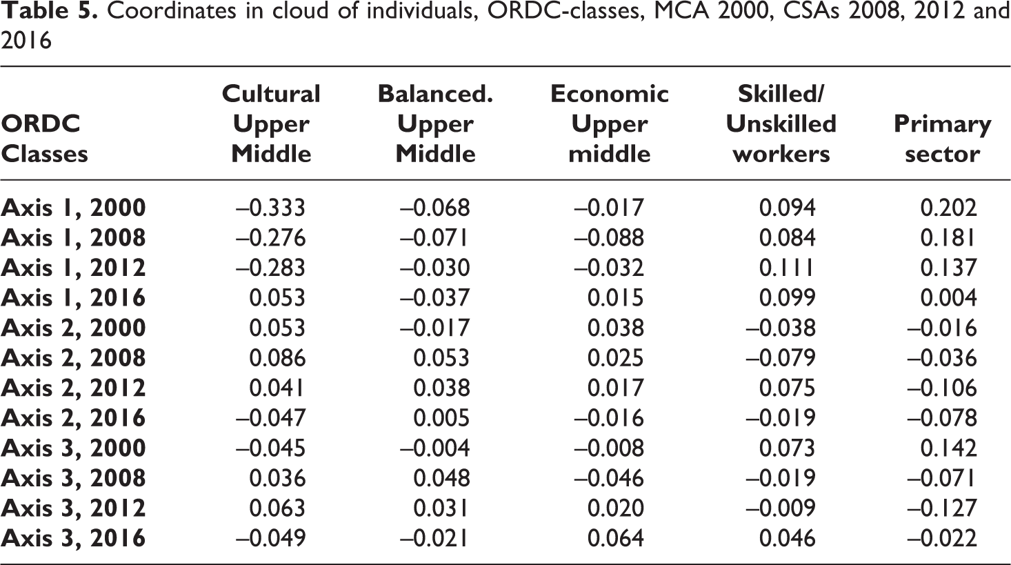
The overall pattern is clearly one of structural stability across time. Despite any variation that might stem from sampling differences, the changes are mainly <.10 from one year to the next.
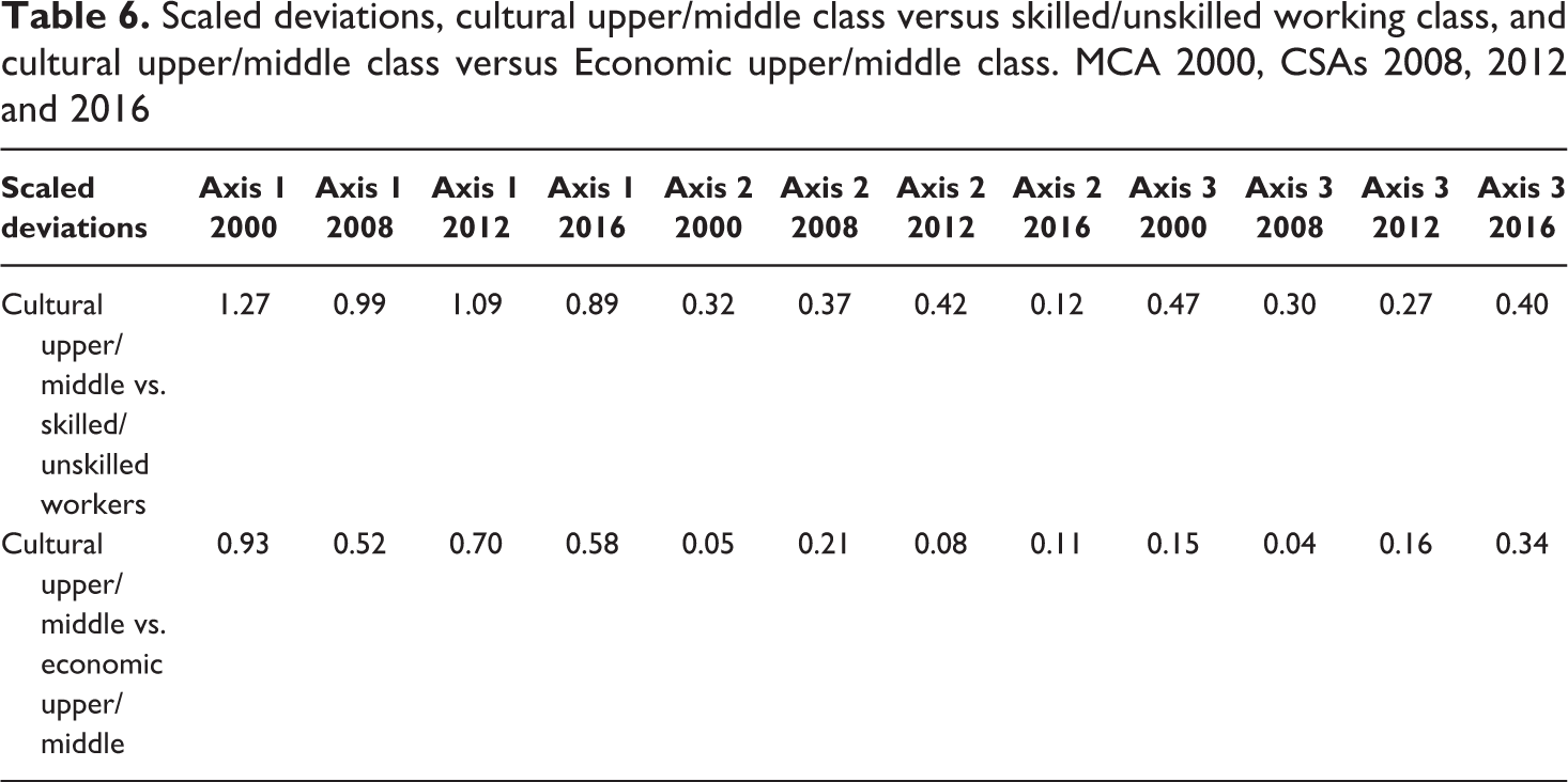
The same pattern of stability is found when examining the scaled deviations 8 between select class categories (see Table 6). The scaled deviation between the cultural upper/middle class and the skilled and unskilled working class is consistently >.90 on Axis 1. We also find that while there was not a notable distance between these class categories on Axis 3 in 2000, it rises just above the threshold for a notable distance in 2008 (.57), and then decrease to .12 in 2016.
The intra-class division along Axis 1, between the cultural and the economic fractions of the upper/middle class, is consistently notable across the period, although the scaled deviations fluctuate between .93 and 0.52.
Scaled deviations, cultural upper/middle class versus skilled/unskilled working class, and cultural upper/middle class versus Economic upper/middle class. MCA 2000, CSAs 2008, 2012 and 2016
Summed up, the results thus indicate both structural stability and structural change. The principal opposition has remained stable over the period we have analyzed, and so is the polarity that can be described as a class hierarchy. The secondary oppositions, axes 2 and 3, have partly changed, but mainly because of increased importance of specific, rather than general media and cultural practices, i.e. a partial and gradual, rather than a global change.
Conclusion
Drawing on Bourdieu’s theoretical-methodological ideas on how cultural divisions are best conceived of as a system of relations between cultural properties, we have presented an alternative approach to study stability and change in cultural divisions across time, as well as stability and change in how such cultural divisions are connected to class divisions. Expanding on recent developments within GDA, we have combined the use of two distinct statistical techniques: MCA and CSA. Whereas CSA has been used in synchronic analyses to assess whether and how the structure of subspaces is similar to or different from other subspaces (and structural wholes) at a given point in time, we have sought to demonstrate how CSA also can be applied in the assessment of structural stability and change across time. By projecting class categories onto our MCA and CSA spaces as supplementary points, the development of how cultural divisions have remained connected to class divisions can be traced across time.
This methodological approach, we would argue, has three promising potentials. Specifically, the approach allows for the systematic investigation of three key aspects: (i) whether and how the dimensionality and the structure of primary axes of geometrical spaces have been stable or subject to change; (ii) the extent to which the oppositions depicted by the axes of such spaces have become weaker or stronger; and (iii), how the connection between cultural divisions and class divisions has developed over time.
Although the main aim of the article has been methodological, our analysis has also sought to contribute to research on the class-lifestyle nexus. First, the analysis indicates both structural stability and change in terms of the connection between cultural divisions and class divisions. Overall, the basic dimensionality of the spaces has remained similar in this period: the CSA spaces display strong resembles to the reference space from 2000. However, the analysis indicates at least some cultural change. Although most of the primary axes in the CSAs appear close to the primary axes in the reference space, some of them rotate slightly away from the original axes. This is particularly the case with Axis 2 and 3. This suggests that some of the specific cultural practices and media preferences that make up the cultural divisions have been subject to change.
Second, the analysis indicates that cultural divisions in terms of cultural participation and media practices are growing increasingly entrenched in Norwegian society: The strength of the oppositions depicted by the primary axes in the CSA spaces grows continuously over the 16-year period under scrutiny. This highlights the point that even if some of the substances involved in the structure of cultural divisions may change, the divisions themselves may nonetheless grow stronger.
Finally, our analysis supports the hypothesis that the homology, or structural connection, between the structure of cultural divisions and the structure of class divisions is steadfast, although some of the specific cultural goods and activities making up the structure of the former have changed over time. The geometrical distances between the upper and lower classes are strikingly similar across the whole period. This contradicts the hypothesis that changes in the content of cultural divisions also implies that the class-lifestyle nexus is gradually crumbling.
Footnotes
Notes
Acknowledgements
We would like to thank two anonymous reviewers and the editors of BMS for constructive criticisms to earlier version of this manuscript. The analyses are done in SPAD and in specialized software for CSA written by prof. Brigitte Le Roux. Neither of the above are responsible for any mistakes we might have done.
Declaration of Conflicting Interests
The authors declared no potential conflicts of interest with respect to the research, authorship, and/or publication of this article.
Funding
The authors received no financial support for the research, authorship, and/or publication of this article.