PHASE: An Open-Source Program for the Analysis of Drosophila Ph ase,A ctivity,and S leep Under E ntrainment

Abstract

The problem of entrainment is central to circadian biology. In this regard, Drosophila has been an important model system. Owing to the simplicity of its nervous system and the availability of powerful genetic tools, the system has shed significant light on the molecular and neural underpinnings of entrainment. However, much remains to be learned regarding the molecular and physiological mechanisms underlying this important phenomenon. Under cyclic light/dark conditions, Drosophila melanogaster displays crepuscular patterns of locomotor activity with one peak anticipating dawn and the other anticipating dusk. These peaks are characterized through an estimation of their phase relative to the environmental light cycle and the extent of their anticipation of light transitions. In Drosophila chronobiology, estimations of phases are often subjective, and anticipation indices vary significantly between studies. Though there is increasing interest in building flexible analysis tools in the field, none incorporates objective measures of Drosophila activity peaks in combination with the analysis of fly activity/sleep in the same program. To this end, we have developed PHASE, a MATLAB-based program that is simple and easy to use and (i) supports the visualization and analysis of activity and sleep under entrainment, (ii) allows analysis of both activity and sleep parameters within user-defined windows within a diurnal cycle, (iii) uses a smoothing filter for the objective identification of peaks of activity (and therefore can be used to quantitatively characterize them), and (iv) offers a series of analyses for the assessment of behavioral anticipation of environmental transitions.

Entrainment to environmental cycles is a key property of circadian clocks and is critical for maintaining the adaptive advantage of rhythmic phenomena across taxa (Pittendrigh, 1981; Vaze and Sharma, 2013). Critical markers of entrainment are (i) the stable and reproducible daily timing of behavior (phase of entrainment), (ii) systematic changes of these phases under various zeitgeber regimes, and (iii) anticipation of predictable environmental transitions (for instance, lights-ON and lights-OFF) (Pittendrigh, 1981; Moore-Ede et al., 1982; Roenneberg et al., 2005). Therefore, measures of phases and estimates of anticipation are critical to characterizing entrained behavior of organisms.

Drosophila has proved to be an insightful model system in which many of the molecular and neuronal underpinnings of entrainment have been revealed, owing to its ease of maintenance, its relatively simple nervous system, and the availability of powerful genetic tools (Hardin, 2011; Helfrich-Förster, 2020). The daily morning and evening peaks of activity are the most prominent features of the Drosophila locomotor activity rhythm under light/dark (LD) cycles. The timing and amounts of activity underlying these peaks are therefore of significant interest to those using the fly to understand entrainment (Hamblen-Coyle et al., 1992; Renn et al., 1999; Grima et al., 2004; Stoleru et al., 2004). Thus, the objective estimation of the phases of these peaks and the extent of their anticipation of environmental transitions is critical for the characterization of the entrained circadian system of flies.

Recently, there has been an increasing interest in the development of open-source software and teaching tools to analyze and understand features of circadian rhythms (Schmid et al., 2011; Cichewicz and Hirsh, 2018; Geissmann et al., 2019; Abhilash and Sheeba, 2019; Cenek et al., 2020; Kostadinov et al., 2021; Hammad et al., 2021). However, to the best of our knowledge, a program that supports the standard analysis and visualization of Drosophila activity and sleep rhythms that is also easily accessible, incorporates objective analysis of phases of activity, and includes measures of anticipation is not currently available. To this end, we present PHASE – a freely available MATLAB program to analyze Drosophila Phase, Activity, and Sleep under Entrainment.

Materials and Methods

PHASE: System Requirements, Installation, and the GUI

PHASE is a freely available, open access, and stand-alone program written for MATLAB and hosted on GitHub (https://github.com/ajlopatkin/PHASE). However, users can also run PHASE in MATLAB, which requires a current MATLAB license (Runtime R2020 or later; The MathWorks, Inc, Natick, MA). The PHASE bundle can be downloaded from GitHub (https://github.com/ajlopatkin/PHASE/tree/master/Installer%20Downloads) and instructions in the supplemental manual can be used to install and run the program on Windows (7 or later) and Mac (10.13 or later) computers. Only data acquired using Drosophila Activity Monitor (DAM) systems via DAMSystem3 and processed using the DAMFileScan can be used as input for PHASE (Trikinetics, Waltham, MA; https://www.trikinetics.com). The DAM system is the most commonly used apparatus for recording locomotor activity in flies and is also widely used to measure sleep in the fly (Chiu et al., 2010; Cichewicz and Hirsh, 2018; Kostadinov et al., 2021).

The graphical user interface (GUI) of PHASE can be divided into 5 sections (Figure 1a). The first is where users choose the directory where all their files for analysis are stored (Figure 1a-i). Input files for the analysis must be DAM-scanned channel files. The second section of the interface is “Data Settings” and is one of the most critical components of PHASE (Figure 1a-ii). From left-to-right, “Data Settings” consists of the following: a display window which lists all the monitors that are available in the user-chosen folder (specified in the first section), a display window showing all the channels within the monitor files, a display window that shows which monitor and channels have been selected by the user for analysis, and input settings for the desired analysis (Figure 1a-ii). Details regarding how to use these input settings are included in the figure legends and the supplemental user manual. The third section is where the user chooses which of the PHASE functions to execute (Figure 1a-iii, 1b and 1c). The user chooses a scaling option for the y-axis in the plots, the folder in which to save all the plots and spreadsheets generated by PHASE, and the name of the output files in section 4 (Figure 1a-iv). The buttons to execute the functions chosen in Figure 1a-iii are in the fifth section of the user interface (Figure 1a-v). The 3 available buttons are “Sleep Analysis”, “Normalized Activity Analysis,” and “Averaged Activity Analysis.” Each of these buttons will use a different data set to perform all the user-chosen analysis. In the case of “Sleep Analysis,” PHASE will use standard sleep data (see Shafer and Keene, 2021). For “Normalized Activity,” PHASE uses activity data normalized to the total activity per cycle, and for “Averaged Activity,” it uses activity data averaged over the length of the user-defined bin (see Figure 1a-iii). We encourage users to read the figure legends and consult the user manual for detailed instructions.

Figure 1.

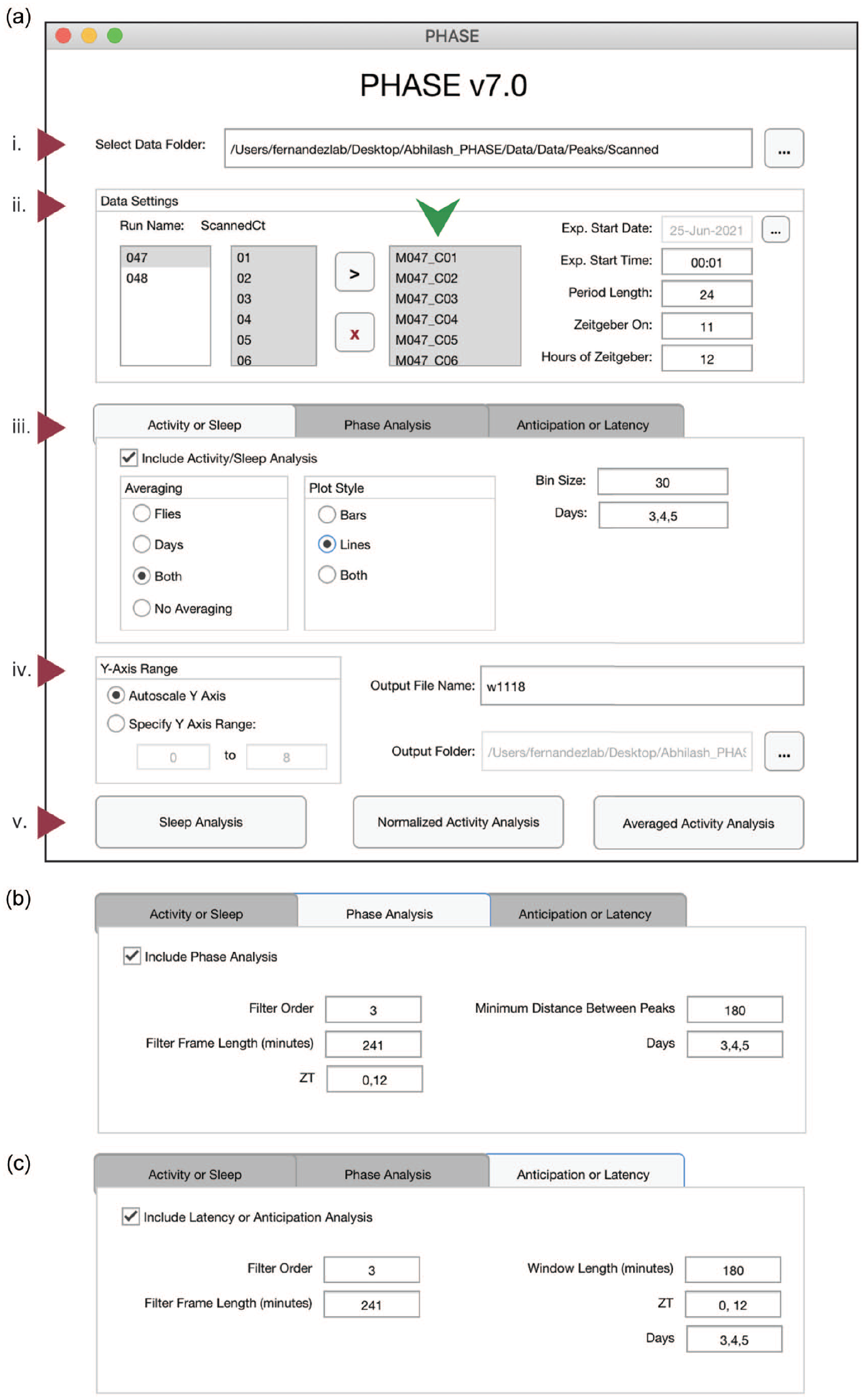
The PHASE graphical user interface. (a) The PHASE window as displayed on startup. The interface can be divided into 5 sections. (i) The “Select Data Folder” dialogue box: users click the button with 3 dots on the right to locate and open the folder containing 1-min scanned DAM channel files for analysis. PHASE automatically detects the monitor numbers and displays all available channels under “Run Name: ScannedCt” in the “Data Settings” section (ii). Users must move the channels to be analyzed by pushing them to the small display window to the right (green arrowhead) using the black “>” symbol. All channels within this box must then be selected for analysis to continue. Monitors must be analyzed one at a time. Experimental (Exp.) Start Date must be indicated by clicking the button with 3 dots in the top-right corner of section (ii). Exp. Start Time must be input in the HH:MM format using military time (00:00-23:59) and must start 1 min after the intended experimental start time. In this example, the experiment would begin at midnight on 25 June 2021. “Period Length” is the length of one full environmental cycle. This defaults to 24 in PHASE but can be adjusted for experiments using non-24-h environmental cycles. “Zeitgeber On” is the time at which experimental Zeitgeber (e.g., light, or high temperature) starts and is indicated as hours after Exp. Start Time. “Hours of Zeitgeber” indicates the duration of the zeitgeber ON time and is expressed in hours. In this example, the lights on period lasted 12 h per cycle, and lights turned on at 1100 h. (iii) The “Analysis” section has 3 tabs. Users can visualize and analyze activity/sleep profiles and export corresponding metrics using the “Activity or Sleep” tab; the timing of daily peaks of activity can be analyzed using the “Phase Analysis” tab (b); and the anticipation of environmental transitions can be analyzed using the “Anticipation or Latency” tab (c). These 3 analysis tabs can be run singly or in any combination. The “Phase Analysis” and “Anticipation or Latency” tabs have distinct interfaces and require the inputs shown in panels (b) and (c). To include these analyses in PHASE output files, the “Include . . . ” box on the top-left of each tab must be checked (iii). For the “Activity or Sleep” analysis, users must also choose the way the data will be averaged (across days, across flies, or both), the plot style (lines or bars), the bin size (in minutes), and the days to be analyzed (separated by commas). In this example (a-iii), we have used 30 min bins and analyzed days 3, 4, and 5. The following inputs described are relevant for both the “Phase Analysis” and “Anticipation or Latency” tabs (b) and (c). The values of these inputs need not necessarily be the same for the 2 options. Filter Order and Filter Frame Length (minutes) inputs pertain to the Savitzky-Golay smoothing filter used for identifying peaks (see text for details). ZT indicates the times of the day around which peaks must be identified (for “Phase Analysis”) or before which anticipation must be quantified (for “Anticipation or Latency” analysis), with ZT00 always defined as the onset of zeitgeber. Multiple ZT values can be provided, separated by commas, to characterize any number of consistently timed peaks or anticipation of environmental transitions within the time series. Days should indicate the days over which phase and/or anticipation or latency must be estimated. These can be different from the days used as input in panel (a-iii). The “Phase Analysis” tab requires an additional input, “Minimum Distance Between Peaks” (b), which must be provided in minutes and is used by PHASE to identify multiple peaks outside this user-defined window. The “Anticipation or Latency” tab has an additional input, Window Length, which is expressed in minutes and sets the window of time prior to the chosen ZTs within which PHASE will estimate anticipation. The “Output” section (iv) has 3 dialogue boxes. The first, “Y-Axis Range” determines if the range of y-axis values in the sleep/activity plots will be set automatically or by user-specified values. The remaining dialogue boxes require the user to the set “Output File Name,” and the “Output Folder,” which determines where output files will be saved. The 3-dot button on the right of the Output Folder dialogue box is where the user navigates to the target. (v) The analysis execution buttons allow to either analyze Sleep, Normalized Activity, or Averaged Activity (see text for details). All the analysis chosen in panels (a-iii, b, or c) will be executed only when 1 of these 3 buttons is clicked. Abbreviations: PHASE = Phase, Activity, and Sleep under Entrainment; DAM = Drosophila Activity Monitor; ZT = Zeitgeber Time. Color version of the figure is available online.

Results

Activity and Sleep Analysis

PHASE allows users to view activity and sleep profiles in ways that facilitate easy visual inspection of inter-individual and cycle-to-cycle variations in temporal patterns (Figures 2 and 3). It also computes and exports all underlying data to spreadsheets that also contain commonly used metrics for assessment of sleep and activity, such as the number of beam crossings (i.e. activity) and the number and duration of sleep bouts in the day and night windows (see manual). Distinct types of sleep and activity plots can be generated in PHASE using different approaches (see Figure 1a-iii): averaging data across flies, days, and/or both (Figures 2a-2c and 3a-3c). When averaging across “Days” is chosen, 1 plot for every individual fly (i.e. channel) is generated wherein activity/sleep is averaged across all cycles indicated by the user (Figures 2a and 3a). PHASE generates 1 PDF file for every 12 channels. Thus, the 32 channels of a standard DAM monitor are saved as 3 PDF files. When averaging across “Flies” is chosen, a single averaged plot of the activity or sleep time series is generated for the days indicated in 1A-iii and data are averaged across all the channels chosen by the user (Figures 2b and 3b). When averaging across “Both,” a single plot of activity/sleep profile is generated, wherein data are averaged across all the days and flies indicated by the user (Figures 2c and 3c).

Figure 2.

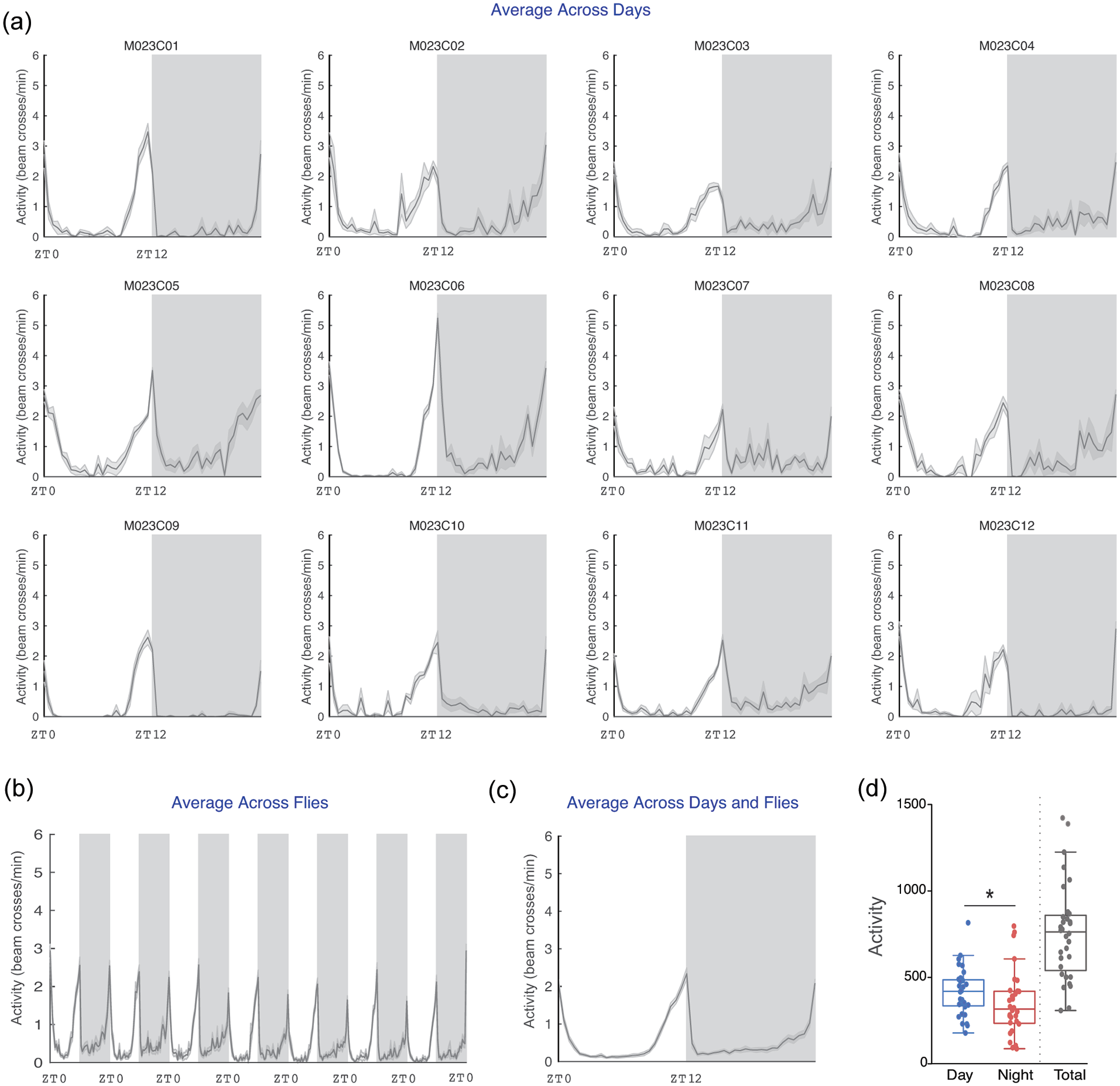
“Averaged Activity Analysis” outputs from PHASE summarizing activity across flies and environmental cycles. Here, example activity time-courses are displayed for male Canton-S (CS) flies recorded under LD12:12 cycles at a constant 25 °C. (a) Averaged activity output from PHASE when time series are averaged across days for 12 individual flies (see panel a-iii in Figure 1). (b) Output from PHASE when time series are averaged across all 32 flies (see panel a-iii in Figure 1). (c) Output from PHASE when time series are averaged across both days and flies (see panel a-iii in Figure 1). Gray-shaded regions in panels (a) through (c) indicate the scotophase (i.e. darkness) of the light/dark cycle. When these analyses are executed, corresponding spreadsheets are generated (see user manual for details), which can be used to visualize and perform statistical tests on activity parameters. One such example is shown in (d), wherein total daytime and nighttime activity in CS flies is compared. As described previously, daytime activity is significantly higher than nighttime activity as judged by a Wilcoxon’s matched pairs test implemented in R (V = 395; p = 0.013; also indicated on the plot using an asterisk). Also shown, for relative comparison, is the total activity counts across 1 full cycle (not included in any statistical comparisons). Note that such plots can be visualized as normalized time series using the “Normalized Activity Analysis” output button (Figure 1a-v). Abbreviation: PHASE = Phase, Activity, and Sleep under Entrainment. Color version of the figure is available online.

Figure 3.

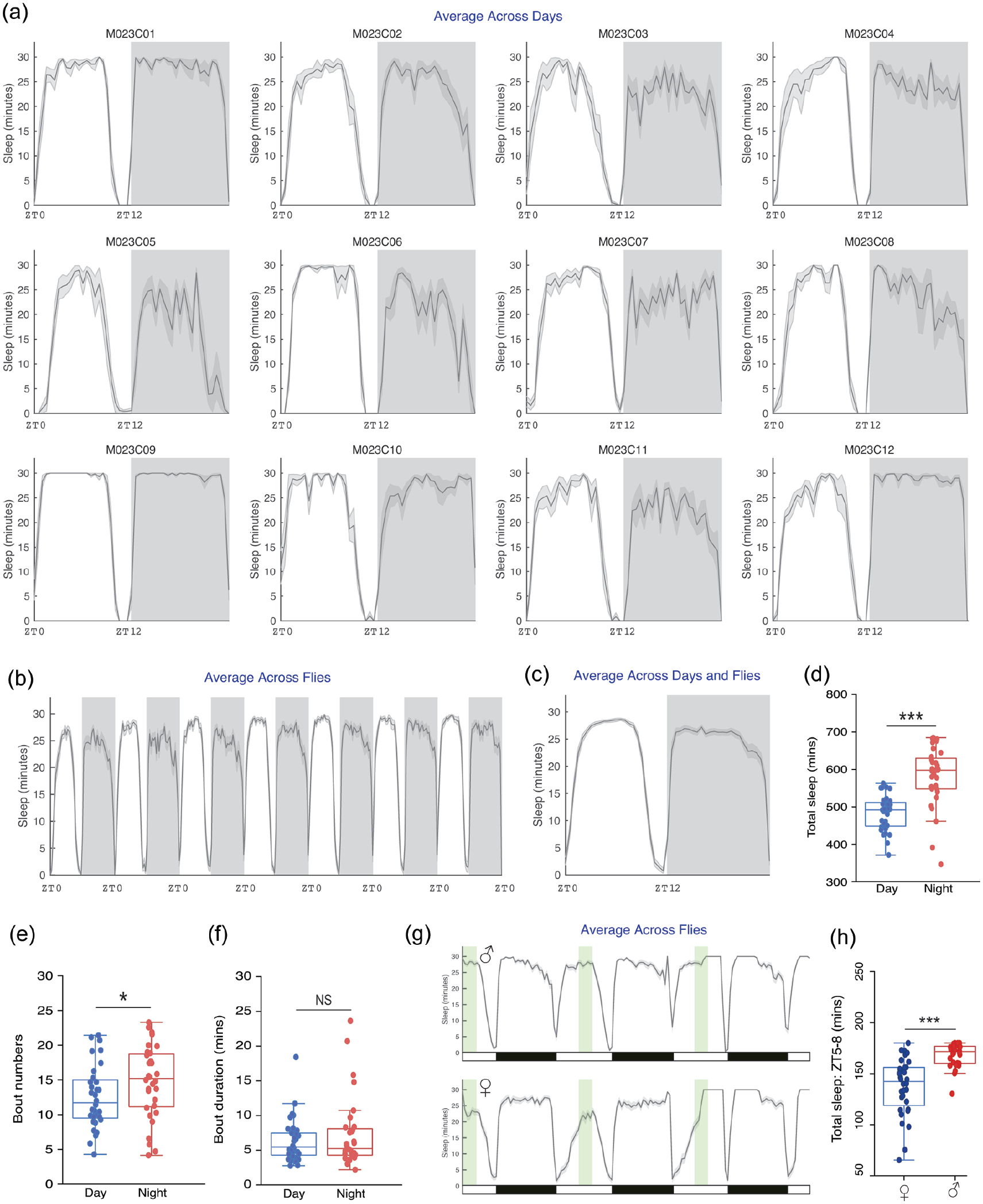
“Sleep Analysis” outputs from PHASE. Shown here are plots of sleep, measured as minutes/user-defined bin, averaged across days for 12 individual flies (a), across all 32 flies (b), and across both days and flies (c) in the same manner as that shown for averaged activity, using the same time series used for the analysis described in Figure 2 (see Figures 1a-iii and 2). Gray-shaded regions in panels (a) through (c) indicate the scotophase of the light/dark cycle. The exported spreadsheets from the PHASE’s sleep analysis were used to compare total sleep, sleep bout numbers and duration across day and night in male CS flies. (d) As previously described, total minutes of sleep is higher during the night (V = 15; p = 6.38e-08). (e) The number of sleep bouts was significantly higher during the night (V = 153.5; p = 0.04). (f) Sleep bout duration was not significantly different between day and night (V = 241; p = 0.68). All statistical inferences in panels (d), (e), and (f) were drawn based on Wilcoxon’s matched pairs tests implemented in R. (g) Also shown are plots of sleep, measured as minutes/user-defined bin, averaged across flies for males (top) and females (bottom) for 3 consecutive LD cycles. To select a 3-h window around ZT06, 3-h was defined as the “Hours of Zeitgeber” and “Zeitgeber On” time was changed accordingly in the “Data Settings” input panel (see Figure 1a-ii). This modified daytime window is shown in green, while the actual LD cycle during the experiment is indicated by the black and white bars underneath the plot. In this window, we quantified total minutes of sleep for females and males. (h) As expected from previous work, total minutes of sleep in this 3-h window was significantly higher in males than in females as judged by a Mann–Whitney U test implemented in R (W = 133.5; p = 3.84e-07). Abbreviations: PHASE = Phase, Activity, and Sleep under Entrainment; CS = Canton S; LD = light/dark; NS = not significant. For all panels: *p < 0.05. **p < 0.01. ***p < 0.001. Color version of the figure is available online.

As previously described by many investigators, activity was significantly higher during the day in wild-type Canton S (CS) male flies under LD12:12 (Figure 2d) and total sleep was higher during the night (Hamblen-Coyle et al., 1992; Majercak et al., 1999; Hendricks et al., 2000; Shaw et al., 2000). Increased nighttime sleep was accompanied by increased bout numbers at night (Figure 3e) with no differences in the bout duration between night and day (Figure 3f). Sexual dimorphism in sleep is well documented (Huber et al., 2004; Andretic and Shaw, 2005), with females sleeping less during the day than males. We quantified sleep within a 3-h window around mid-day (ZT05-ZT08) to highlight how window-specific analysis of sleep/activity can be carried out using PHASE (Figure 3 g). As expected, this analysis revealed that daytime sleep was significantly higher in males than in females (Figure 3 h).

Savitzky-Golay Filtering for the Quantification of Behavioral Phase

One of the earliest methods used to objectively characterize the timing of activity peaks in Drosophila was described by Hamblen-Coyle et al. (1992). These authors employed a Butterworth filter to remove high-frequency components of beam crossing time-course data and used a search algorithm to look for peaks within specific windows of interest from the filtered data. Other objective measures have included the use of a non-recursive digital filter (Helfrich-Förster, 1998) and dual smoothing (non-recursive digital filter + moving averages) (Rieger et al., 2003). Recent studies have used various alternative methods of peak detection (Potdar and Vasu, 2012; De et al., 2013; Das et al., 2015; Liang et al., 2019), which supports the need for a robust peak detection method and software to implement it. While it is useful to use smoothed data to quantify the timing of behavioral peaks, there are limitations to using filters like the Butterworth because such filters work well only for stationary time series (wherein frequency and amplitude are maintained from cycle-to-cycle). Behavioral rhythms are typically non-stationary and therefore require tools that work well for such time series (Leise, 2013, 2017). One such digital filter is the Savitzky-Golay (SG) filter (Savitzky and Golay, 1964; Schafer, 2011). The SG filter is known for its ability to preserve amplitude of the signal while de-noising the data set, thereby making it extremely useful for the identification and characterization of peaks and the estimation of their phases. While it has been used in other sub-disciplines of biology (Azami et al., 2012; Chu et al., 2014), it has not, to our knowledge, been applied to circadian data.

Mathematically, the SG filter fits a polynomial of order p, to a window of size n over the original time series using linear least squares. This window of the time series then slides across the entire length of the time series, fitting a polynomial of order p for each window. In the case of equally spaced data, as is the case with Drosophila activity and sleep time series, there exists an analytical solution to this set of least squares equations as a single set of convolution coefficients, thereby making this a fast and computationally straightforward filter. These coefficients can then be used to derive signal estimates (e.g., activity or sleep) at a given time t. This smoothed, estimated signal can then be used to make peak calls and characterize anticipation of environmental transitions (see below). For its implementation in PHASE, it is important to note that the sliding window must consist of an odd number of time points, whose units must be in minutes.

To demonstrate the effect of polynomial order and window length on smoothing, we used SG filters with varying values of p and n and overlaid smoothed estimates over the raw data (Suppl. Fig. S1). These results show that, for a given filter order, increasing window lengths results in smoother time series. Furthermore, for a given window length, increasing the filter order increases the ability of the filter to capture nuances of the time series (Suppl. Fig. S1). Therefore, the most useful filter order and frame length will depend on the nature of both the raw data and the question being posed, which can be established using an iterative process to determine the most appropriate parameters. As an example, we have documented the phases of morning and evening peaks of activity, the associated inter-individual variation, and the amplitude of morning and evening peaks of CS males under LD12:12 at 25 °C using different polynomial orders (p) and filter frame lengths (n) (Suppl. Tables S1-S3). It is immediately clear that although the mean values of morning and evening peak phases do not vary much, the coefficients of variation across individual flies differ vastly. For instance, lower polynomial orders and longer filter frame lengths have higher inter-individual variation, which may indicate that phase calls were made with reduced accuracy (Suppl. Tables S1 and S2). In the case of amplitude, the maximum activity counts around the morning and evening peaks of activity in the average profile were 1.48 and 2.11/min. From Supplementary Table S3, it is clear that lower and higher polynomial orders and filter frame lengths, in most cases, provide estimates of amplitude that are further away from the actual values of activity. Using such measures, users could vary the polynomial order and filter frame length to determine which combinations best capture their raw data most closely and use that for downstream analyses.

We used a filter order of 3 and a frame length of 241 min to estimate peak times in the analysis presented here to illustrate how this filter can be used to characterize activity peaks in Drosophila behavioral time series (employing the iterative approach discussed above). Filtering with these parameters captures the activity patterns of wild-type CS males entrained to 3 LD cycles of differing day lengths well (Figure 4a-left). For equinox and short-day cycles (LD 8:16, 8 h of light and 16 h of darkness), the morning peaks of activity immediately follow lights-on but occur about an hour after lights-on under long-day conditions (Figure 4b). Evening peaks of activity are clearly adjusted to occur just before dusk (Figure 4c) in CS males, as previously described (e.g. Qiu and Hardin, 1996). In contrast, per ⁰¹ mutants, which lack a functional molecular clock, are characterized by evening peaks that occur after lights-off under all day lengths (Figure 4a-right and 4c), suggesting that these are masked peaks of activity and not clock-driven activity peaks. This illustrates the utility of the SG filter for determining if behavioral peaks anticipate or follow environmental transitions.

Figure 4.

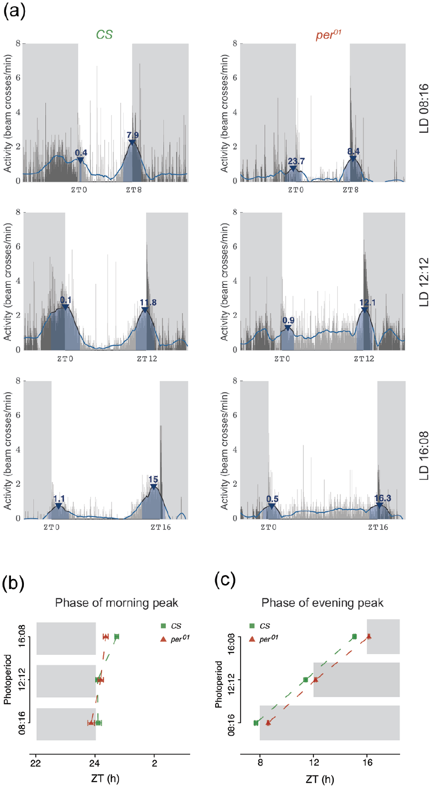
“Phase Analysis” outputs from PHASE. (a) Representative activity of CS male flies under LD08:16 (top-left), LD12:12 (middle-left), and LD16:08 (bottom-left), and per ⁰¹ flies in the same 3 regimes (right). In all cases, the thin gray vertical bars show the activity of the fly in 1-min bins averaged across all days chosen by the user. The blue line is the smoothed waveform produced by the Savitzky-Golay filter (see text for details). Peaks are identified based on the smoothed waveform represented by the blue line and are indicated by the blue arrowheads. Annotated above the arrowheads are the phases of the identified peaks expressed as ZTs. The blue-shaded region under the arrowhead is the width of the peak. Also shown are mean ± SEM (standard errors of the mean) of the phases of morning (b) and evening (c) peaks of activity for CS and per ⁰¹ flies under the 3 photoperiods. Gray-shaded regions in both (b) and (c) indicate the scotophase of the light/dark cycle in their respective photoperiod regimes. Abbreviations: PHASE = Phase, Activity, and Sleep under Entrainment; CS = Canton S; ZT = Zeitgeber Time; LD = light/dark. Color version of the figure is available online.

We used a second fly mutant to demonstrate the utility of the SG filter in the characterization of behavioral timing. As previously shown, pdf ⁰¹ mutants have an advanced evening peak of activity and a reduced or absent morning peak of activity under LD cycles (Renn et al., 1999). Comparing the top and bottom rows of Figure 5a reveals that the morning peaks of activity are highly reduced in pdf ⁰¹ flies compared with their genetic control background, w ¹¹¹⁸ . We extracted peak information with PHASE using the order and window length values described above and quantified both the phases and heights of activity peaks for both genotypes. As expected from previous work (Renn et al., 1999), the morning peaks of pdf ⁰¹ mutants were delayed (Figure 5b) and their heights significantly reduced (Figure 5c), whereas the evening peak phases were significantly advanced (Figure 5d) and their heights significantly reduced compared with w ¹¹¹⁸ controls (Figure 5e). These examples further illustrate the utility of smoothing time series data with the SG filter to characterize the timing and magnitude of activity peaks. A similar approach can be used to estimate and characterize peaks of sleep in flies using PHASE.

Figure 5.

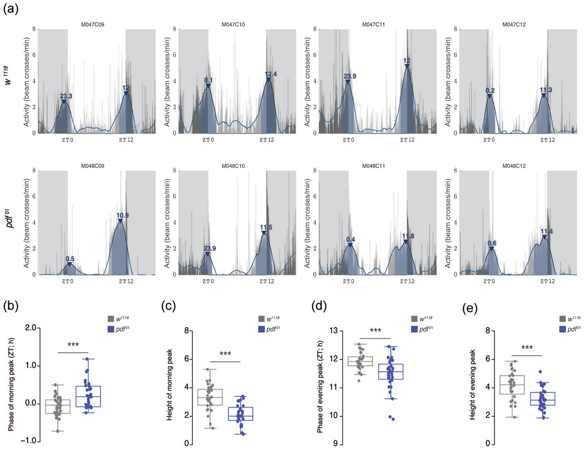
Characterization of activity peaks in pdf ⁰¹ mutants. (a) Representative activity profiles of 4 males each of w ¹¹¹⁸ controls (top) and pdf ⁰¹ mutants (bottom) overlaid with Savitzky-Golay-filtered waveforms show advanced evening peaks and reduced morning peaks in pdf ⁰¹ flies. We quantified phases and heights of both morning and evening activity peaks and found that phase of morning peak is significantly delayed in pdf ⁰¹ flies (b; W = 264.5; p = 0.0009), and the height of morning peak is significantly lower compared with w ¹¹¹⁸ flies (c; W = 879; p = 1.581e-07). On the other hand, the phase of evening peak is significantly advanced (d; W = 794.5; p = 0.0001521) and its height significantly lower (e; W = 800; p = 6.718e-05) in pdf ⁰¹ mutants compared with w ¹¹¹⁸ flies. Comparisons were done using Mann–Whitney U tests implemented on R. Abbreviation: ZT = Zeitgeber Time. *p < 0.05. **p < 0.01. ***p < 0.001. Color version of the figure is available online.

The Use of Slopes for Estimating Anticipation

The behavioral anticipation of predictable environmental transitions depends on a functional and entrained circadian system. One of the first methods of estimating anticipation was proposed by Stoleru et al. (2004) who used an estimate of anticipation that was directly proportional to the gradual, stepwise increase in activity prior to environmental transitions, and inversely proportional to the startle response due to the transition. Only a few studies have made use of this method (Stoleru et al., 2004, 2007; Sheeba et al., 2010). A simpler approach to the estimation of anticipation was proposed by Harrisingh et al. (2007), who used the ratio of activity in a 3-h window before a transition of interest and the activity in a 6-h window before the same transition. The expected value of this metric in case of a complete lack of anticipation is 0.5. As anticipation increases, the value of this metric is also expected to increase. This approach has been used in many studies (Im and Taghert, 2010; Sheeba et al., 2010; Potdar and Vasu, 2012; De et al., 2013; Prakash et al., 2017; Baik et al., 2018; Schlichting et al., 2019). A recently published approach to quantifying anticipation made use of slopes from least squares linear regression modeling of the increase in activity before specific environmental transitions (Fernandez et al., 2020). While both the above discussed measures of anticipation can be easily calculated from the activity data exported by PHASE, the slope method requires additional steps. We therefore implemented slope calculations into our analysis package to ease the use of this approach for Drosophila behavioral time series data.

For the calculation of slopes, PHASE allows users to choose the duration of the time-window and the temporal resolution of time series data sets to conduct linear regression analysis. Using this method, we compared the activity of wild-type (CS) and per ⁰¹ mutant males in the hours before lights-on and light-off under LD12:12 cycles. Best fitting lines for each fly reveal that CS flies (Figure 6a) display steeper increases in activity (i.e., higher slopes) before both the morning and evening transitions compared with per ⁰¹ mutants (Figure 6b). We quantified morning and evening slopes for every fly and compared average slope values for each genotype. The results revealed that, as expected, per ⁰¹ mutants do not display significantly positive slopes in the hours leading to light transitions, indicating that there is no morning or evening anticipation, consistent with the absence of circadian timekeeping (Figure 6c and legend therein). Furthermore, CS flies consistently displayed significantly positive slopes that were on average much higher than those of per ⁰¹ flies, consistent with the presence of robust anticipatory activity in CS controls (Figure 6c). It is important to note here that this functionality is available only for the “Averaged Activity Analysis” option (see Figure 1a-v) and not for the “Normalized Activity Analysis” option. It is also useful to contrast this method to the method of estimating anticipation described by Harrisingh et al. (2007). We found that using Harrisingh’s method for per ⁰¹ mutants indicates anticipation in both morning and evening windows. Furthermore, while CS flies did not show higher anticipation than per ⁰¹ flies in the morning window, they had higher statistically significant anticipation index compared with per ⁰¹ flies in the evening window (Suppl. Fig. S2). These results show that, at least in this context, the slope method of estimating anticipation is better at capturing the differences between mutants and controls than the previously used metrics of anticipation.

Figure 6.

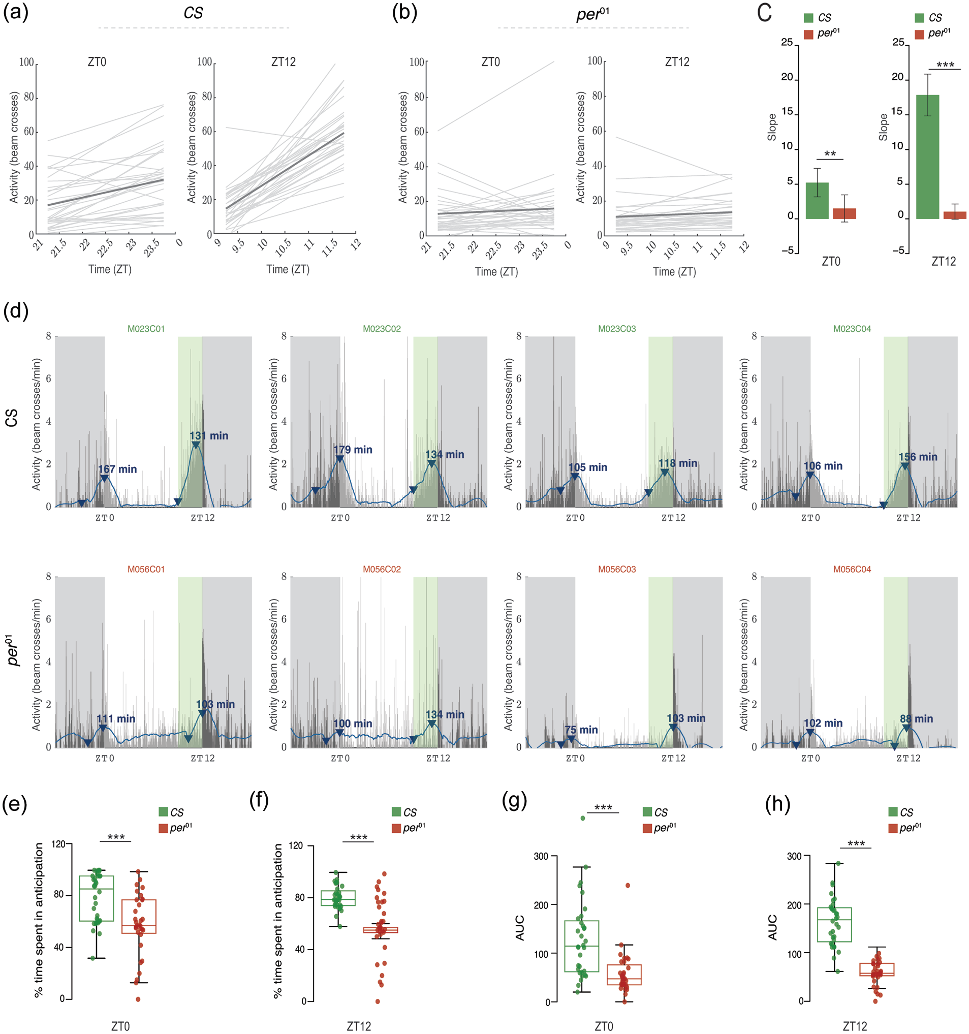
“Anticipation or Latency” outputs from PHASE. Plots indicating slopes of activity levels in user-defined windows for individual male CS (a) and per ⁰¹ (b). Light gray lines represent least squares linear regressions for individual flies, and the dark gray line represents the averaged regression across all flies. (c) The slope values represented in panels (a) and (b) are exported within a PHASE-generated spreadsheet and are used to making comparisons between genotypes or treatments. A population with no anticipation would be expected to show a slope of zero. We performed single-sample t tests to determine if the mean slope for each genotype was different from zero. CS flies have slope values that are significantly greater than zero in both the morning (left; t₃₁ = 5.2057; p = 1.191e-05) and evening (right; t₃₁ = 12.051; p = 3.118e-13) windows. On the other hand, per ⁰¹ flies did not have significant anticipation in the morning (left; t₃₁ = 1.564; p = 0.128) or evening (right; t₃₁ = 1.928; p = 0.063) window. The error bars on these plots are 95% confidence interval (CI) based on the reported t tests. Therefore, any mean with error bars that cross the zero-mark is not different from zero. We also performed Welch’s t tests to compare anticipation values between CS and per ⁰¹ flies in both windows. We found that anticipation in the morning (left; t_61.87 = 2.686; p = 0.009) and evening (right; t_39.04 = 10.669; p = 3.912e-13) windows is significantly greater in CS flies as compared with per ⁰¹ mutants. (d) Representative activity profiles (channels 1 through 4) of CS (top) and per ⁰¹ (bottom) flies under LD12:12. The thin vertical bars represent the activity of the fly in 1-min bins averaged over all days chosen by the user. The blue line is the smoothed waveform after applying a Savitzky-Golay filter (see text for details). Gray–shaded region is the scotophase of the light/dark cycle. The green-shaded region in the plot (clearly visible before ZT12) is the user-defined window in which anticipation/latency is computed. This green-shaded region is not an output of PHASE and has been shown here only for illustration. The blue arrowheads show the minimum and maximum value of activity on the smoothed waveform in the user-defined window. Note that the arrowhead is not displayed for smoothed data points that are negative. The arrowhead marking the maximum value is annotated with the duration of anticipation or latency (in minutes; in other words, duration between the minimum and maximum value). (e-f) Percentage of time spent in anticipation is significantly higher in CS than per ⁰¹ flies in both the morning (e; ₁χ² = 13.052; p = 0.0003) and evening (f; ₁χ² = 40.713; p = 1.763e-10) windows. Similarly, AUC were also significantly higher in CS than per ⁰¹ flies in morning (g; ₁χ² = 19.043; p = 1.278e-5) and evening (h; ₁χ² = 37.324; p = 1e-09) windows. All inferences in panels (b) through (e) were made using Kruskal-Wallis tests implemented in R. For all panels: *p < 0.05, **p < 0.01, ***p < 0.001. Note that a similar approach can be used on sleep data to summarize increases in sleep following environmental transitions as a means of quantifying the latency of sleep (see manual). Abbreviations: PHASE = Phase, Activity, and Sleep under Entrainment; CS = Canton S; CI = confidence interval; AUC = areas under the curve; ZT = Zeitgeber Time. Color version of the figure is available online.

The SG filter can also identify the highest and lowest points of activity in the smoothed data within the user-defined window (Figure 6d). PHASE uses these values to estimate the duration of anticipatory activity and the area under the curve between the minimum and maximum data points identified by PHASE (Figure 6d). Based on these measurements (see manual for details), we found that the percent time spent in anticipation was significantly higher in CS controls compared with per ⁰¹ mutants for both morning (Figure 6e) and evening (Figure 6f) transitions. We also found that the area under the curve was significantly larger for CS controls for both transitions (Figure 6 g and 6 h), consistent with significantly reduced anticipation in per ⁰¹ mutants. In addition, the slope method is utilized by PHASE to calculate anticipation of environmental transitions for “Normalized Activity” and latency of sleep following environmental transitions using the smoothed normalized activity and sleep data, respectively (see manual for details). We note that each method of measuring anticipation has its own set of limitations and the ability to implement multiple measures in a program like PHASE will be helpful for researchers interested in quantitatively characterizing anticipation in fly behavioral time series.

Discussion

In conclusion, we offer PHASE as a platform to support the visualization and analysis of behavioral time series through user-defined, window-based measurements of activity and sleep data. Furthermore, PHASE implements a powerful smoothing filter to model fly activity and sleep rhythms, which allows for the quantitative characterization of activity peaks and anticipation, a feature that is not currently widely available. All codes for PHASE are open-source and available at: https://github.com/ajlopatkin/PHASE. The software bundle for installation can be downloaded from the same link. A detailed user manual is available as supplementary online material. This user manual contains detailed information regarding the interface, suggestions to make analyses easier, details about the graphs generated, and descriptions of common errors and how to troubleshoot them, all of which we hope will make this program useful for the circadian fly community and support future breakthroughs in our understanding of circadian entrainment.

Supplemental Material

sj-docx-1-jbr-10.1177_07487304221093114 – Supplemental material for PHASE: An Open-Source Program for the Analysis of Drosophila Phase, Activity, and Sleep Under Entrainment

Supplemental material, sj-docx-1-jbr-10.1177_07487304221093114 for PHASE: An Open-Source Program for the Analysis of Drosophila Phase, Activity, and Sleep Under Entrainment by J. L. Persons, L. Abhilash, A. J. Lopatkin, A. Roelofs, E. V. Bell, Maria P. Fernandez and Orie T. Shafer in Journal of Biological Rhythms