Sage Journals: Discover world-class research

Abstract

The daily proportion of light and dark hours (photoperiod) changes annually and plays an important role in the synchronization of seasonal biological phenomena, such as reproduction, hibernation, and migration. In mammals, the first step of photoperiod transduction occurs in the suprachiasmatic nuclei (SCN), the circadian pacemaker that also coordinates 24-h activity rhythms. Thus, in parallel with its role in annual synchronization, photoperiod variation acutely shapes day/night activity patterns, which vary throughout the year. Systematic studies of this behavioral modulation help understand the mechanisms behind its transduction at the SCN level. To explain how entrainment mechanisms could account for daily activity patterns under different photoperiods, Colin Pittendrigh and Serge Daan proposed a conceptual model in which the pacemaker would be composed of 2 coupled, evening (E) and morning (M), oscillators. Although the E-M model has existed for more than 40 years now, its physiological bases are still not fully resolved, and it has not been tested quantitatively under different photoperiods. To better explore the implications of the E-M model, we performed computer simulations of 2 coupled limit-cycle oscillators. Four model configurations were exposed to systematic variation of skeleton photoperiods, and the resulting daily activity patterns were assessed. The criterion for evaluating different model configurations was the successful reproduction of 2 key behavioral phenomena observed experimentally: activity psi-jumps and photoperiod-induced changes in activity phase duration. We compared configurations with either separate light inputs to E and M or the same light inputs to both oscillators. The former replicated experimental results closely, indicating that the configuration with separate E and M light inputs is the mechanism that best reproduces the effects of different skeleton photoperiods on day/night activity patterns. We hope this model can contribute to the search for E and M and their light input organization in the SCN.

Keywords

photoperiodism mathematical modeling computer simulations circadian oscillator evening and morning oscillators suprachiasmatic nucleus synchronization

Natural environments undergo cyclic seasonal changes in biotic and abiotic factors throughout the year. Accordingly, organisms have evolved seasonal adjustments in physiology and behavior associated with these changes (Baker, 1938), such as seasonal reproduction, migration, and hibernation. Synchronization of these seasonal phenomena is attained by diverse annual environmental cues that serve as natural calendars. One of these cues is photoperiod, the daily proportion between light and dark hours within the 24-h light/dark cycle (Bradshaw and Holzapfel, 2007; Fig. 1A, top). Thus, given the regularity of photoperiodic changes that recur from year to year, many organisms have evolved the ability to interpret photoperiod and use it as a highly reliable anticipatory cue for future seasonal conditions (Bradshaw and Holzapfel, 2007).

Figure 1.

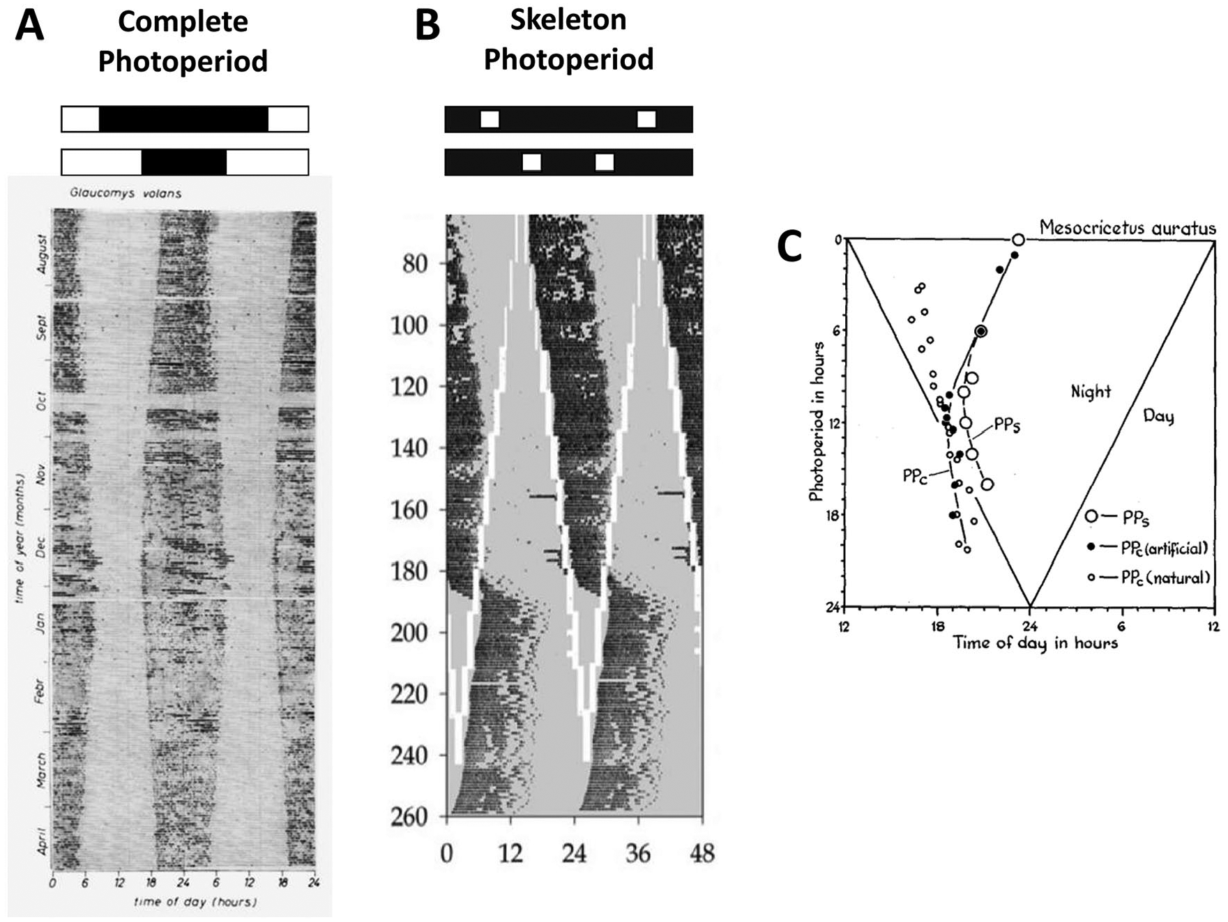
Examples from the literature of activity patterns under varying photoperiods. (A) Double-plotted actogram depicting the 9-month activity record (black marks) of a nocturnal flying squirrel (Glaucomys volans) exposed to natural, complete photoperiod variation schematized on top. Each line represents 48 h of data, and the vertical axis shows consecutive days, one below the other. Daily activity duration (α) parallels the length of the dark phase. (B) Double-plotted actogram depicting the activity record (black marks) of a mouse exposed to varying skeleton photoperiods, as schematized on top, in which 2 light pulses (white) occur daily on a darkness background (gray). The interpulse interval (“night” interval) that contains the activity phase is progressively shortened throughout the days. α is gradually compressed on days 140 to 180. Thereafter, the phase of entrainment is reversed to the complementary interpulse interval (psi-jump), and α is decompressed. (C) Phase of daily activity onset of hamsters (Mesocricetus auratus) exposed to different photoperiods. PPc, complete photoperiod; PPs, skeleton photoperiod. A: Daan and Aschoff (1975); B: Spoelstra et al. (2014); C: Pittendrigh and Daan (1976a). (A) Reprinted by permission from Springer Nature: Oecologia. Circadian rhythms of locomotor activity in captive birds and mammals: their variations with season and latitude. Daan S and Achoff J, 1975. (B) Reprinted by permission from Taylor & Francis Ltd (http://www.tandfonline.com): Chronobiology International. Compression of daily activity time in mice lacking functional Per or Cry genes. Spoelstra K, Comas M, and Daan S, 2014. (C) Reprinted by permission from Springer Nature: Journal of Comparative Physiology A: Neuroethology, Sensory, Neural, and Behavioral Physiology. A functional analysis of circadian pacemakers IV: entrainment: pacemaker as clock. Pittendrigh CS and Daan S, 1976.

In addition to its role as seasonal synchronizer, photoperiod variation also has profound effects on the day/night patterns of activity on a 24-h scale (Pittendrigh, 1988). As reported in different species, 2 parameters of daily activity are modified along with the day-to-day changes in photoperiod: activity duration (time between daily activity onset and offset, α) and its phase of entrainment (time between a reference phase in the light/dark cycle and a reference phase in the activity rhythm, ψ). For instance, in day-active (diurnal) animals, α lasts longer during spring/summer than on winter/autumn days. This has been reported in different vertebrate species exposed to natural photoperiods, for example, grizzly bears (Ware et al., 2012), squirrels (Wauters et al., 1992; Williams et al., 2012), birds (Daan and Aschoff, 1975), and humans, as inferred from sleep duration (de la Iglesia et al., 2015; Yetish et al., 2015). The inverse is observed for night-active (nocturnal) animals, which present a shorter activity phase in the spring/summer, as reported for a few rodents (Boulos and Macchi, 2005; Daan and Aschoff, 1975; Kenagy, 1976) and bats (Erkert, 2000). Representative data from a nocturnal rodent in Figure 1A illustrate the photoperiod-dependent changes in α (Daan and Aschoff, 1975).

As for ψ, it is remarkably fixed when photoperiod is varied in the vicinity of LD12:12, as shown in data from hamsters in Figure 1C in the interval LD9:15 to LD15:9. Activity onset occurs shortly after lights-off, independent of photoperiod. The same has been observed in flying squirrels (DeCoursey, 1972). For these and other nocturnal animals, this means that activity onset is locked to dusk, whatever the timing of dusk throughout the seasons; this is an adaptive strategy from the ecological point of view (Pittendrigh and Daan, 1976b). However, experiments with systematic photoperiod manipulation have shown that the tight phase association between activity onset and dusk is lost under extreme, long or short days (Elliott, 1976). This is illustrated in the extreme values of Figure 1C. Our aim is to understand complex response patterns such as the abrupt phase changes and α modulations displayed in Figure 1, using mathematical modeling and computer simulations. Our simple model is based on physiological and anatomical knowledge of the circadian system that has been accumulated over decades. Our objective is to indicate the minimum elements of this system that are sufficient to process the length of the day throughout the year.

In mammals, a circadian oscillator located in the hypothalamic suprachiasmatic nuclei (SCN) has a dual role in mediating the photoperiodic transduction on physiology and behavior (Coomans et al., 2015; Goldman, 2001). On one hand, it generates daily activity rhythms in behavior that display photoperiod-dependent patterns, as indicated above. On the other hand, it shapes photoperiod-dependent melatonin profiles that relay time-of-year information to the hypothalamus-hypophyseal axis for control of seasonal phenomena (Ikegami and Yoshimura, 2012; Illnerová and Vaněček, 1982). These 2 functions are achieved through a reorganization of the SCN internal structure as the photoperiod changes (Buijink et al., 2016; Ciarleglio et al., 2011; Evans et al., 2013; Mrugala et al., 2000; Schwartz et al., 2001; Sumová et al., 1995; Tackenberg and McMahon, 2018; VanderLeest et al., 2007). While the first function evokes day-to-day responses on activity patterns, the second allows anticipatory initiation of cascades of developmental and reproductive processes that culminate in seasonal events distant in time. In this work, we focus on the first function and pursue how daily locomotor activity is affected by different photoperiods.

In the 24-h time scale, the circadian oscillator/pacemaker in the SCN is entrained by the daily light/dark cycle, via direct neuronal inputs from the retina (Abrahamson and Moore, 2001). To explain how this entrainment mechanism could account for daily activity patterns under different photoperiods, Pittendrigh and Daan (1976b) proposed that the pacemaker could be composed of 2 coupled oscillators. The oscillators have been named “evening” (E) and “morning” (M). The authors proposed that this qualitative dual-oscillator model could potentially account for photoperiodic changes in α if one oscillator tracked dawn (M) and the other tracked dusk (E), changing the phase relationship to one another throughout the year.

Although the E-M model has existed for more than 40 years, its physiological bases are still not fully resolved (Daan et al., 2001; de la Iglesia et al., 2000 Helfrich-Förster, 2009; Inagaki et al., 2007; Yoshikawa et al., 2017), and it has not been quantitatively tested under varying photoperiods using mathematical models. For instance, it is still not clear to what extent 2 SCN components separately entrained by dawn and dusk are necessarily required for photoperiod encoding, both from the physiological and from the dynamical points of view.

To better explore this proposition, previous studies have recorded daily activity rhythms of rodents exposed to skeleton photoperiods (Pittendrigh and Daan, 1976a; Spoelstra et al., 2014). Instead of a full light/dark cycle, this protocol consists of 2 light pulses given at the times corresponding to the transitions between the light and dark phases of the full cycle (Fig. 1B, top). Therefore, photoperiod is modeled as the ratio of the 2 intervals between “dawn” and a “dusk” light pulses. Despite the simplicity of skeleton photoperiods, they are sufficient (1) to adjust reproductive function according to the seasons (Milette and Turek, 1986; Wade et al., 1986) and (2) to induce daily changes in α according to photoperiod (Pittendrigh and Daan, 1976a; Spoelstra et al., 2014; Takahashi and Menaker, 1982).

When exposed to skeleton photoperiods, animals always concentrate daily activity in one of the darkness intervals between light pulses, which is assigned the “night interval” for nocturnal species. Whether activity occurs in the longer or the shorter interval between pulses depends on previous light conditions and on the relative lengths of the intervals. Curiously, for nocturnal animals, when α is gradually compressed by reducing the current night interval, the activity phase eventually shifts to the complementary interval, thus inverting the day and night references of the cycle (Fig. 1B). This inversion of the phase of entrainment ψ (psi) is denoted “psi-jump” (Pittendrigh and Daan, 1976a). Critically, before the psi-jump, the activity phase tracks one pulse of the skeleton photoperiod and, afterward, it tracks the opposite pulse (Fig. 1B).

Modeling efforts have been made before to understand E and M dynamics in constant conditions (Daan and Berde, 1978; Kawato and Suzuki, 1980; Oda and Friesen, 2002; Oda et al., 2000). Other studies have modeled entrainment of a single oscillator (Pittendrigh and Daan, 1976b; Schmal et al., 2015) or very complex oscillator networks (Taylor et al., 2017) under different photoperiods. In the present study, we simulate a system of 2 coupled limit-cycle oscillators under skeleton photoperiod manipulations and seek minimal configurations that could display photoperiod dependent α compression and psi-jump. To our knowledge, this is the first attempt to explicitly model E and M dynamics in the context of photoperiodism.

Materials And Methods

To investigate the effects of photoperiod on the E-M model, we used 2 coupled nonlinear limit-cycle oscillators, governed by the Pittendrigh-Pavlidis equations. These equations have been previously used to model circadian rhythms in Drosophila (Pittendrigh, 1981; Pittendrigh et al., 1991) and the E and M oscillators in rodents (Oda and Friesen, 2002; Oda et al., 2000). Each oscillator is described by a set of 2 equations (1-4). Following previous conventions (Oda et al., 2000), the terms from E and M oscillators are identified by subscribed letters.

Evening oscillator (E):

d R_{E} / d t = R_{E} - c_{E} S_{E} - b_{E} S_{E} 2 + (d_{E} - L) + K

(1)

d S_{E} / d t = R_{E} - a_{E} S_{E} + C_{M E} S_{M}

(2)

Morning oscillator (M):

d R_{M} / d t = R_{M} - c_{M} S_{M} - b_{M} S_{M} 2 + (d_{M} - L) + K

(3)

d S_{M} / d t = R_{M} - a_{M} S_{M} + C_{E M} S_{E}

(4)

State variables R and S together describe the state of one oscillator at a given time point. The R variable is prevented from reaching negative values. Parameters a, b, c, and d are set to fixed values and collectively define an oscillator configuration, with intrinsic period and amplitude. K (Kyner) is a small nonlinear term that guarantees numerical smoothness (K = k₁/(1 + k₂R²), k₁ = 1, k₂ = 100; Oda et al., 2000). The L term simulates the light input (forcing variable). Its value is maintained at zero to simulate the dark hours. When lights are turned on, it is changed to a positive amplitude value in arbitrary units (a.u.), which simulates the light intensity. In one particular case indicated below, we used pulses of negative amplitude. The coupling term C controls the strength with which the E oscillator influences the morning oscillator (C_EM) and vice versa (C_ME). When coupling is symmetric, C_EM = C_ME.

In most cases, we used a standard configuration (a = 0.85, b = 0.3, c = 0.8, d = 0.5), previously employed to model circadian rhythms in rodents (Oda et al., 2000). Other configurations have been explored to investigate the dependence of phenomena on the period and amplitude of oscillators (see the supplemental materials). Computer simulations were performed in the CircadianDynamix extension of the Neurodynamix II software (Friesen and Friesen, 1994) using the Euler method for numerical integration, with 1000 integration steps per 24 h.

In our simulations, we portray the phases of the circadian oscillators (squares and triangles) and of the behavioral rest/activity rhythm (black bars) separately (Fig. 2), to emphasize the temporal interdependence between oscillator and behavioral activity. In Figure 2, we explicitly show how the phases corresponding to activity were transduced from the phases of the circadian oscillator. This was achieved by defining a threshold, which was set to 40% of the state variable amplitude. Whenever the S variable of either oscillator went above its threshold, the model organism was considered as resting (activity was inhibited); otherwise, it was considered as active. Thus, in the dual-oscillator model, the total activity band was determined by E and M together (Fig. 2), with activity set in antiphase to the peak amplitude of the circadian oscillators. This is equivalent to the phase relationship between behavioral activity and peak SCN electrical discharge in nocturnal mammals (Houben et al., 2009).

Figure 2.

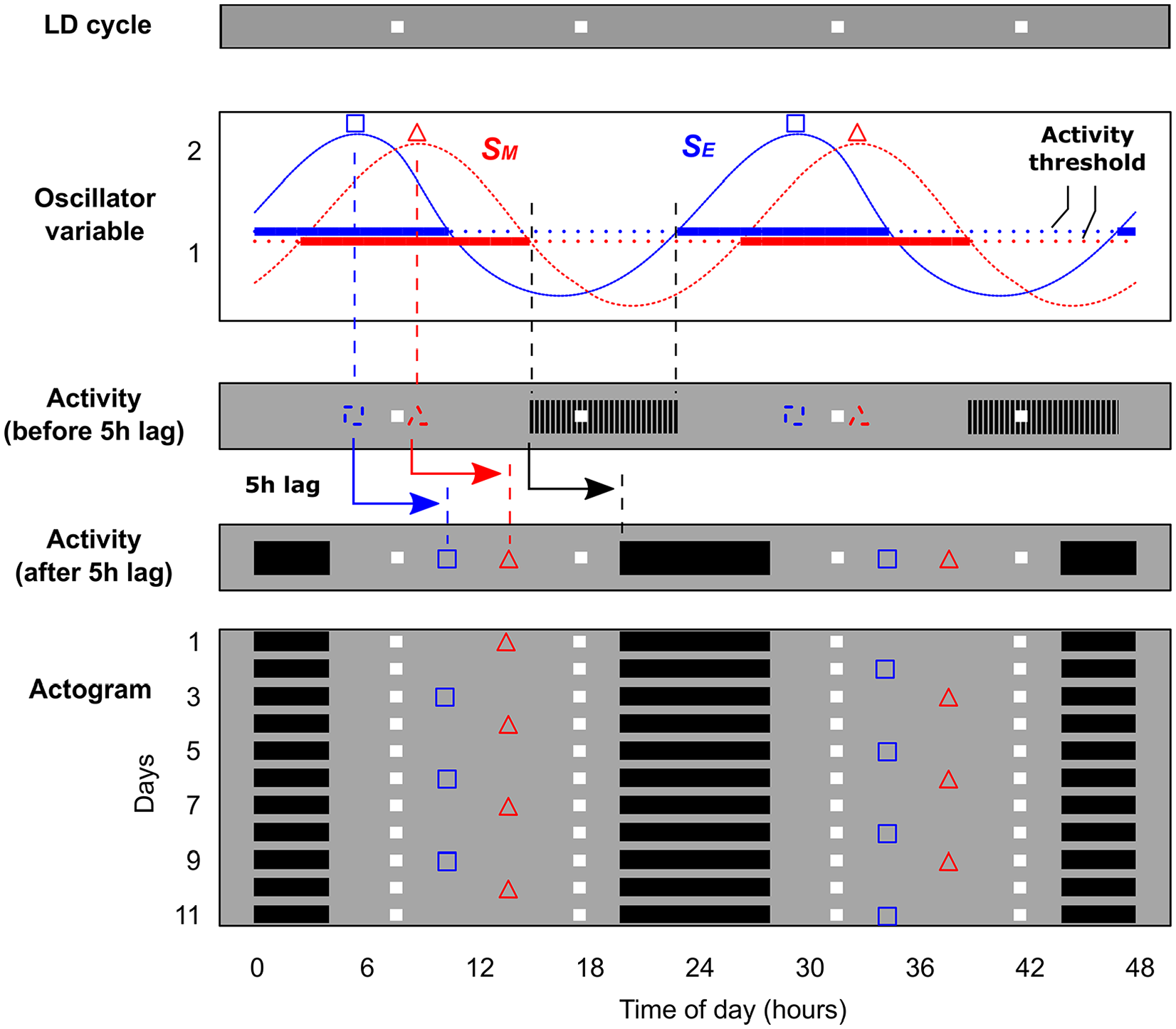
Conversion of oscillators’ state variables to daily activity/rest rhythms in the simulated animal. The process is illustrated for a 48-h section of a simulation record. The oscillator is exposed to skeleton photoperiods indicated by “LD cycle” at the top, with white squares representing light pulses in a darkness (gray) background. The state variable S from the evening (S_E) and morning (S_M) oscillators is recorded continuously and compared with the activity thresholds. The peaks of the state variables are also recorded and represented as squares (evening) and triangles (morning). Whenever the state variables from both oscillators are below the threshold, the model animal is considered active; otherwise, it is set as inactive. This preliminary activity phase as well as the state variable peaks are represented by dashed symbols in the section “Activity (before 5h lag).” The pulses of the skeleton photoperiod are indicated as white squares. An addition step is made to better fit the phase to experimental data reported in the literature. We set a 5-h lag (arrows) to the composite phases of oscillators and activity, relative to the light-dark cycle, as indicated in “Activity (after 5h lag).” The data for consecutive days is plotted one day below the other in the “Actogram.” Each day represents 48 h of data, with days 1 to 2 in the first line, 2 to 3 in the second line, and so forth. In the actogram, state variable peaks are shown only every 3 days to make visualization easier. Color versions are available online.

Finally, an extra step was added in the simulations to better fit experimental data for nocturnal animals under skeleton photoperiods. The composite phases of oscillators and activity were delayed by 5 h throughout all simulations, establishing an interval lag relative to the light signal. Importantly, we maintained the same fixed phase relationship between oscillators and activity rhythm (Fig. 2). This step was necessary because although activity patterns in the simulations matched closely to experimental data, there was a discrepancy between the exact time of their occurrences. This discrepancy was resolved by setting a phase difference between the light pulses and the simulated oscillator.

The daily light/dark cycle was modeled as a skeleton photoperiod, with 2 light pulses every 24 h (Fig. 1B, top; Pittendrigh and Daan, 1976a; Spoelstra et al., 2014). We simulated 4 configurations of the model to represent different putative physiological mechanisms (Fig. 3, top). As a control, in model I, we first simulated a single oscillator subjected to the skeleton photoperiod (isolated E, with null coupling; Fig. 3A, top). All of the remaining configurations had both E and M oscillators, with symmetric coupling. In model II, each of the 2 pulses of the skeleton photoperiod was applied to only 1 of the oscillators (Fig. 3B, top). In model III, both pulses were applied to both oscillators (Fig. 3C, top). Finally, in model IV, the M oscillator received pulses with negative amplitude (Fig. 3D, top).

Figure 3.

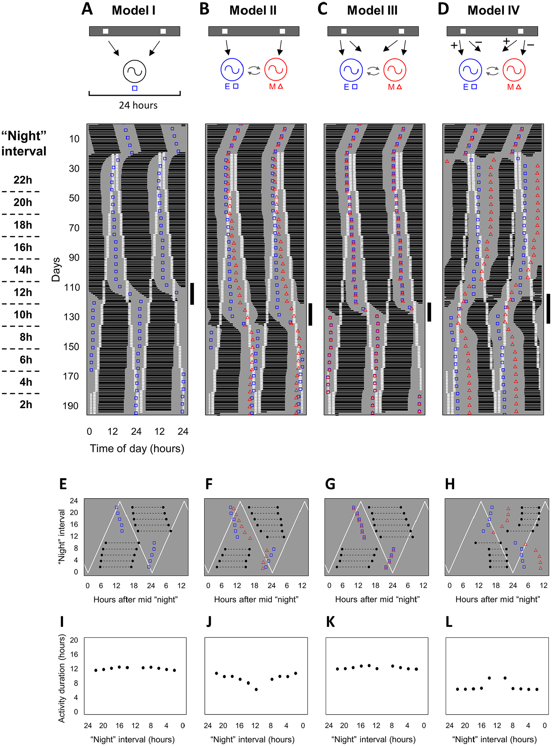
Four configurations of the model and their entrainment to different photoperiods. (A-D, top) Schematic representation of model configurations depicting the skeleton photoperiods (gray-white bars), the oscillators (circular symbols), and the effects of the light pulses on the oscillators (arrows). When 2 oscillators are present (models II-IV), curved arrows indicate coupling between them. (A-D, bottom) Double-plotted actograms illustrating the activity rhythm of the model organism. Plotting conventions are the same used in Figure 2. (A) Model I, single oscillator responsive to both pulses of the skeleton photoperiod. (B) Model II, each oscillator is responsive to one of the pulses of the skeleton photoperiod. (C) Model III, both E-M oscillators respond to both pulses of the skeleton photoperiod. (D) Model IV, same as previous model, except that the M oscillator receives pulses of negative amplitude (−), while the E oscillator receives regular pulses of positive amplitude (+). The days during the psi-jump are highlighted with a vertical line on the right of each actogram. (E-L) Phase of entrainment and activity duration of the 4 model configurations, under different skeleton photoperiods. Measurements were taken on the last day of exposure to each photoperiod, with stable entrainment of the activity rhythm. (E-H) Phase of entrainment. The times of activity onset and offset (black-filled circles) are measured relative to the midpoint of the interpulse interval, in a circular scale (x-axis). Onset and offset points are connected by a black dashed line. Diagonal white lines indicate the times of the pulses, as the skeleton photoperiod changes in the y-axis. Peaks of the state variables are indicated for the evening (squares) and morning (triangles) oscillators in each photoperiod. (I-L) Activity duration (α) under different photoperiods. Entrainment was not stable (missing points) at 12-h “night” intervals in E, H, I, and L and at 10-h “night” intervals in F, G, J, and K. In all versions of the model, oscillators have the standard configuration: a = 0.85, b = 0.3, c = 0.8, d = 0.5. Coupling is symmetric and positive (C_EM = C_ME = 0.07). Pulse duration: 1 h; pulse amplitude: 1.1 or −1.1 (arbitrary units). Color versions are available online.

A model in which one oscillator receives light input and the other does not was not considered, because the light-insensitive oscillator would just passively follow the phase of the sensitive one, with negligible changes in the phase relationship.

The 4 configurations of the model were exposed to different skeleton photoperiods, with different intervals between the daily light pulses. Intervals were reduced from 22 to 2 h, in 2-h steps applied sequentially, each for 15 days. Importantly, this 15-day interval ensures the end of transients and that the entrainment phase achieved by the circadian oscillator is the steady-state phase for each different photoperiod. The lengths of the intervals were measured from the beginning of the first pulse to the beginning of the second pulse. On the last day of exposure to each photoperiod, we measured α and the phase of entrainment. α was measured as the interval between the daily onset and the daily end of activity. The phase of entrainment was measured as the interval between the midpoint of pulses and 2 reference phases of the rhythm, activity onset and offset, and then converted to the 0- to 24-h circular scale.

Simulation Results

We tested the photoperiodic response of the 4 putative models. When exposed to different skeleton photoperiods, all configurations of the model are successfully synchronized to 24 h. Representative actograms are shown in Figure 3A-D (bottom). For the single oscillator in model I (Fig. 3A), only the E oscillator is simulated. The actogram in Figure 3A (bottom) depicts a daily activity band in black, with the 2 pulses of the skeleton photoperiod in white and the oscillator variable peaks as empty squares. We assign “dusk” to the pulse that is locked to activity onset and “dawn” to the other pulse. When the “night” interval between pulses is decreased from 22 to 14 h, the onset of activity remains phase locked to the dusk pulse. This is summarized in Figure 3E, which shows the phase of entrainment quantified on the last day of exposure to each photoperiod. With a single oscillator, there is no noticeable change in α between photoperiods, as observed in the actograms (Fig. 3A, bottom) and quantifications (Fig. 3I). When the interval between pulses is decreased to 12 h, a psi-jump is observed (Fig. 3A, bottom), and from that point onward, the activity onset follows the dawn pulse of the skeleton photoperiod (Fig. 3A, bottom; Fig. 3E). In summary, with 1 oscillator, we can observe the psi-jump phenomenon, but α remains unchanged throughout different photoperiods.

Having observed the behavior of a single oscillator, we can then explore putative E-M mechanisms. In model II, the actogram depicts the activity band, together with squares and triangles representing E and M state-variable peaks, respectively (Fig. 3B, bottom). For simplicity, we chose to model a completely symmetric system in terms of oscillators and coupling, which leads to an overlap between E and M peaks in constant conditions (Fig. 3B, bottom), as reported previously (Oda and Friesen, 2002). When the system is exposed to different photoperiods, again, the activity onset is phase locked to the dusk pulse, up to the 12-h “night” interval (Fig. 3B, bottom; Fig. 3F). Furthermore, the E and M peak phases separate from each other upon initiation of the skeleton photoperiods (squares and triangles in Fig. 3B, bottom), and this becomes more pronounced as the “night” interval between pulses is decreased from 22 to 12 h (Fig. 3B, bottom). Consequently, there is a corresponding decrease in α (Fig. 3B, bottom; Fig. 3J). When the interval between pulses is further decreased to 10 and then 8 h, there is a psi-jump (Fig. 3B, bottom; Fig. 3F). After this, α is gradually increased (Fig. 3J), and the activity onset tracks the opposite, dawn pulse of the skeleton photoperiod (Fig. 3F). These results indicated that model II accounts for photoperiod-induced α adjustments.

One feature observed experimentally in α adjustments is the maintenance of α on the first days after an animal is released in constant darkness from a photoperiod protocol (Pittendrigh and Daan, 1976a). We released the oscillators of model II in constant conditions, after being held in different photoperiods, and observed that α was very similar on the first day. Throughout the days in constant conditions, α gradually lengthened to a steady-state value (Suppl. Fig. S1).

We then explored variations in the coupling strength between E and M in model II (Fig. 4). With very weak coupling, each oscillator tracks one of the pulses, following the pulse times almost passively (Fig. 4A). This results in a great modulation of α (Fig. 4A). Upon a slightly stronger coupling (Fig. 4B), the oscillators remain closer together in the more extreme photoperiods, with a more stable and larger α when the interval between pulses is too long. As the “night” interval between pulses is changed to intermediate photoperiods, E and M separate from each other, and α is modulated (Fig. 4B). With stronger coupling, higher than the standard value used in Figure 3B, E and M stick together throughout most photoperiods (Fig. 4C, D), initially following the dusk pulse and then shifting to the opposite pulse. Consequently, α remains more stable throughout photoperiods. Strikingly, when we compare the weaker coupling with the stronger ones, there is a change in the threshold photoperiod before the psi-jump. With weaker coupling, psi is reversed when the “night” interval between pulses is set to 10 h (Fig. 4A, B), whereas with higher coupling strengths, the psi-jump happens at “night” intervals of 8 and 6 h (Fig. 4C, D).

Figure 4.

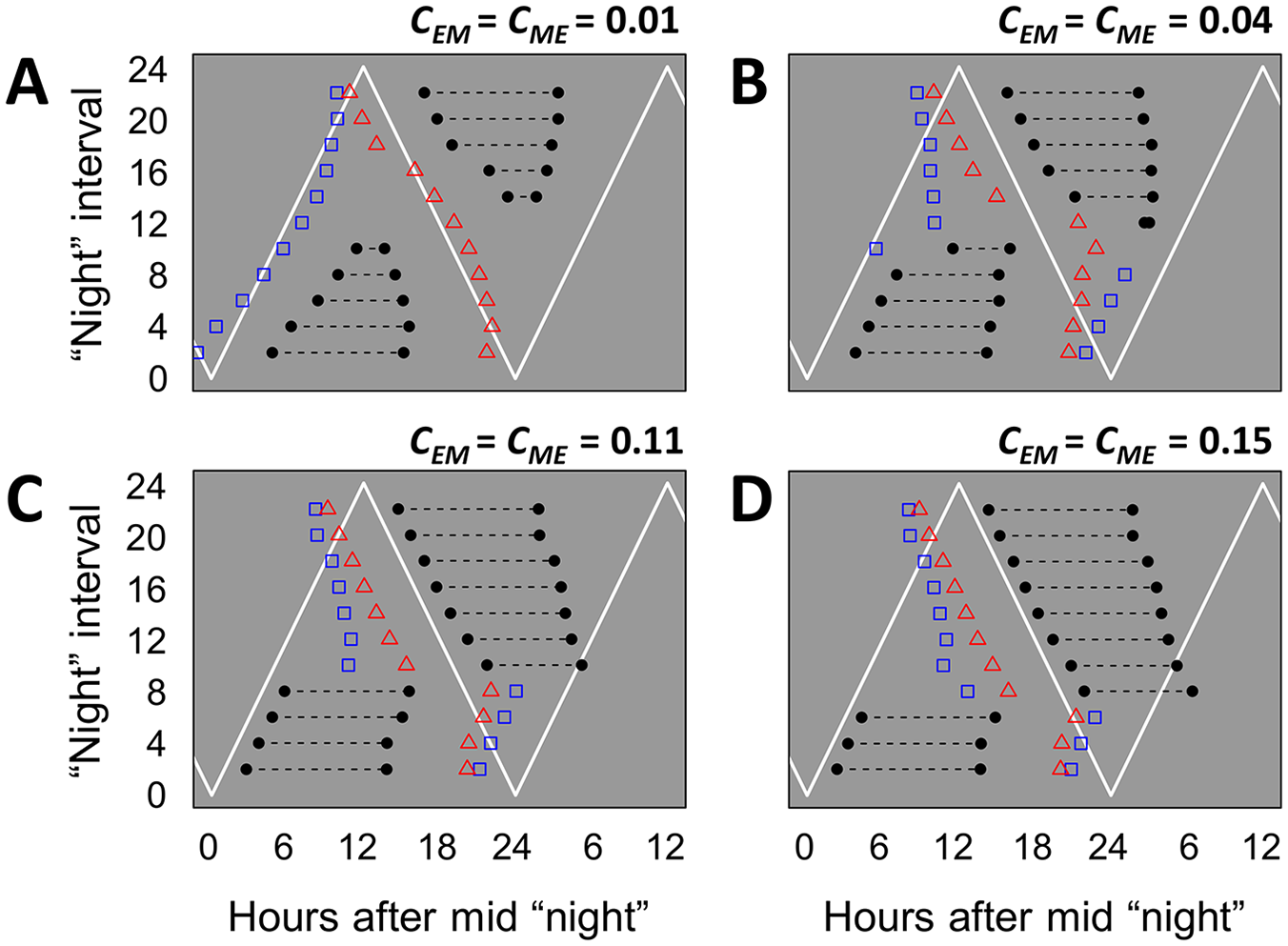
Effects of the coupling strength between evening (E) and morning (M) on the phase of entrainment for model II (Fig. 3B, top). Graphs are plotted following the same conventions of Figure 3E-H. (A-D) Different (symmetric) coupling strengths, as indicated above the graphs. Other model parameters as in Figure 3. Coupling determines how independently the phases of the oscillators change with different photoperiods. Coupling also affects the threshold photoperiod before the psi-jump. Color versions are available online.

The E-M model above is responsive to photoperiod variations; however, it would imply that, in the SCN, distinct subregions corresponding to E and M responded separately to dawn or dusk inputs. Alternatively, it is possible that E and M subregions are equally responsive to dawn and dusk stimuli. To test this hypothesis, in model III, we again have a completely symmetric set of E and M oscillators, but both oscillators are directly synchronized by both pulses of the skeleton photoperiod (Fig. 3C, top). When exposed to the different photoperiods, the E and M phases remained completely overlapped, as seen from the squares and triangles (Fig. 3C, bottom). This overlap remained regardless of the interval between pulses (Fig. 3C, bottom). As a result, α remained basically unchanged (Fig. 3K). The psi-jump occurred just like in the previous versions of the model (Fig. 3G). In short, a completely symmetric E-M model behaves essentially as the single oscillator, when both E and M are equally responsive to the pulses of the skeleton photoperiod. We then hypothesized that if a phase difference between E and M existed in model III, it could generate different responses to light. As reported previously (Oda et al., 2000), a phase difference can generate separate responses to single light pulses in a DD background (Elliott and Tamarkin, 1994). To this end, simulations were performed with an asymmetric configuration. We used 2 oscillators with different intrinsic periods (Suppl. Fig. S2A, B), which results in a basal phase difference in constant conditions (Suppl Fig. S2C). Despite this basal phase difference, E and M phases still overlap in the presence of 2 light inputs in a model III configuration (Suppl. Fig. S2C, D). As shown in Supplemental Figure S2E, each individual oscillator, when isolated, presents very similar phases of entrainment to the different skeleton photoperiods. This explains why, in the coupled system, the phases of the 2 oscillators are brought together by the pulses. Thus, model III does not allow independent E and M shifts that could generate α changes.

The original E-M conceptual model suggested that the component oscillators should have different intrinsic properties, such as period and phase response to light (Pittendrigh and Daan, 1976a, 1976b). As a result, each component oscillator would phase lock to a different pulse of the skeleton photoperiod. As the interval between pulses changed with different photoperiods, the oscillators would tend to separate from each other and promote α adjustments. In the asymmetric E-M case described above, however, both oscillators tracked the dusk pulse, despite their asymmetries (Suppl. Fig. S2E). In this sense, we hypothesized that a fourth version of the model could be made responsive to photoperiodic variations if we added novel, specific asymmetries between E and M, so that each oscillator would track a different pulse of the skeleton photoperiod when isolated.

After several attempts, as described in the supplemental material (and Suppl. Figs. S3–8), we arrived at model IV (Fig. 3D, top). Model IV is a variation of model III, in which the M oscillator receives negative pulses. This guarantees that the isolated E and M go to opposite directions when the photoperiod is changed, because of a change in the phase response to the pulses (Suppl. Fig. S8). When isolated, E behaves as the single oscillator in Figure 3A, following the dusk pulse, while M follows the dawn pulse (Suppl. Fig. S8). In the coupled system (Fig. 3D, top), the free-running rhythm is again equivalent to E-M models II and III (Fig. 3D, bottom). After exposure to skeleton photoperiods, the E and M activities separate (Fig. 3D, bottom). Moreover, the phase relationship between E and M is adjusted with varying intervals between pulses (Fig. 3D, bottom). Hence, there is a change in α, especially in photoperiods close to the 12-h interval (Fig. 3L). As with all previous models, the compound system first tracks one pulse, then there is a psi-jump when the “night” interval is decreased beyond 10 h, and the system tracks the opposite pulse (Fig. 3H). Altogether, these results indicate that the addition of specific asymmetries can rescue a photoperiodic response in a coupled E-M model in which both oscillators are directly synchronized to both pulses of the skeleton photoperiod.

Model Limitations

Our dual-oscillator model, with only 2 emergent components, has been enough to coordinate our understanding of photoperiod-induced α changes and psi-jumps, which are phenomena observed at the behavioral level. However, several experiments at the neural level indicate that the photoperiodic adjustments in the rhythm of the compound nuclei result from the phase distribution of the rhythms from single SCN cells or subregions composed of groups of cells (Brown and Piggins, 2009; Buijink et al., 2016; Inagaki et al., 2007; Jagota et al., 2000; Naito et al., 2008; Rohling et al., 2006; Schaap et al., 2003; VanderLeest et al., 2007; Yoshikawa et al., 2017). It is likely that E and M correspond to SCN subregions, formed by coherent groups of cells. The particular properties of each oscillator may arise not only from variations in intracellular mechanisms (Nuesslein-Hildesheim et al., 2000) but also from differences in intercellular coupling within cell groups (Evans et al., 2013; Farajnia et al., 2014; Lucassen et al., 2012). A model that included changes in single-cell and oscillator network properties could certainly contribute to elucidating the explicit mechanisms and refined aspects of photoperiod encoding in multioscillatory organs. For example, an in silico study on evolving genetic networks suggests that a greater complexity (more oscillators and interactions) can be advantageous for a proper response to photoperiod when it is accompanied by noise fluctuations in environmental light (Troein et al., 2009).

Different photoperiods impose modifications within the fine structure of circadian oscillators, which persist under constant conditions (Mrugala et al., 2000). For instance, pineal glands from birds, explanted in vitro, express melatonin patterns that match the previous photoperiodic conditions experienced by the animals in vivo (Brandstätter et al., 2000). In mammals, it has been shown that, unlike the wild-type mice, vasoactive intestinal polypeptide (VIP) knockout mice fail to display aftereffects of entrainment to different photoperiods (Lucassen et al., 2012). Since VIP is a peptide that promotes interneuronal coupling in the SCN, this indicates that cell-to-cell communication is indispensable for endogenous encoding of photoperiodic information. These examples strongly imply that photoperiod coding has long-lasting effects, likely involving coupling reorganization within the cellular population that comprises the circadian clocks. Buijink et al. (2016) reported greater period instability in Per2::Luc rhythms of individual cells in the mouse SCN on long days versus short days, which further indicates a photoperiod-dependent change in coupling strength.

Coupling changes certainly entail oscillator amplitude changes (Oda et al., 2000), which in turn affect the clock phase-response curve to light (Lakin-Thomas et al., 1991). The ultimate mechanism behind photoperiod encoding could possibly lie on the seasonal modulation of the clock responses to light inputs (Evans et al., 2004; Pittendrigh et al., 1991). In this sense, the model proposed in the present work could be refined by splitting E and M into a distinct subpopulation of oscillators and manipulating individual coupling parameters in a complex neuronal network. This strategy was used by Taylor et al. (2017) to model different regions of the SCN, and they found a mild photoperiodic modulation in the phase difference between the regions. In their case, however, only one region received light inputs, which may explain the lack of pronounced photoperiodic effects.

Finally, our models do not consider the interaction of a homeostatic sleep drive and a circadian oscillator (Borbély et al., 2016; Deboer, 2018) in determining activity onsets and offsets under different photoperiods. Although prior activity is known to affect sleep propensity, several studies have indicated that the timing of sleep under different photoperiods is more strongly determined by the circadian pacemaker. In rats, sleep deprivation under different photoperiods is compensated for on the next day by different sleep compositions, with little change in sleep timing (Franken et al., 1995). In Borbély and Neuhaus (1978), the timing of sleep and wake onsets on the first day of abrupt photoperiod change was still shaped by the photoperiod of the previous day. Trachsel et al. (1986) showed that this also happens in rats released into constant darkness. We recognize that a sleep homeostat could potentially refine timing of activity. Thus, the model could be further complemented by the addition of a homeostatic oscillator. However, we would still consider a system composed of 2 coupled circadian oscillators to explain the complex dynamics of activity onsets and offsets in different light conditions.

Discussion

From an ecological viewpoint, it is tempting to interpret the duration of daily activity in different seasons as a direct response of organisms to the availability of favorable conditions for activity along the 24 h (Bennie et al., 2014). For instance, compression of daily activity in diurnal organisms during autumn/winter can be viewed simply as a reaction to fewer available light hours or to the concentration of warm temperatures around noon. However, laboratory studies with photoperiod manipulations have established that seasonal variation in α has an endogenous component, as shown by the establishment of nonlinear α and ψ variations when photoperiod is varied linearly (Fig. 1B, C; Elliott, 1976). Understanding the mechanisms of photoperiod dependence in α and ψ is still a challenge that requires mathematical modeling. It has been proposed that, in mammals, photoperiod variations of daily activity patterns involve (at least) 2 oscillators, E and M, which control activity onset and offset and are differentially entrained by dawn and dusk (Pittendrigh and Daan, 1976b).

In the mammalian circadian system, the SCN mediates photoperiodic adjustments in activity α; therefore, the nuclei have been strong candidates for the physical substrate of the E and M oscillators (Daan et al., 2001; Helfrich-Förster, 2009). The SCN functions as an overt oscillatory unit, expressing a 24-h profile in multiunit electrical activity (Houben et al., 2009). The duration of this high-electrical-activity state depends on the length of the photophase (reviewed in Coomans et al., 2015) and is mirrored in the daily α duration of overt activity rhythms (Houben et al., 2009) and melatonin profiles (Illnerová and Vaněček, 1982).

Our quantitative analysis of putative E-M models is an attempt to elucidate the requirements of the dual-oscillator system, which allows a response to different photoperiods. The general model predictions should be valid, irrespective of the precise tissue/cellular correspondence, as long as E and M behave as limit-cycle oscillators. In the current study, we searched for model configurations that presented the experimentally observed responses to (skeleton) photoperiods (Fig. 1B). After changes in the interval between pulses, a successful model should present (1) photoperiod-driven adjustments in α, with one oscillator tracking dawn and the other tracking dusk, and (2) a psi-jump after the interpulse interval reaches a threshold duration.

One emergent feature of all simulations is that when 2 light pulses are applied per day, the phase of the oscillator system tracks one of the pulses and remains this way upon systematic changes in the interval between pulses, until a certain threshold value. After this threshold, it tracks the other pulse, and the transition of these 2 regimes occurs abruptly, resulting in a psi-jump. This is true for a 1- or 2-oscillator system and independent of the configurations that were tested (Fig. 3E-H). The switch in the pulse association is typical of models with 2 zeitgeber inputs when the phase difference between them is systematically varied (Oda and Friesen, 2011), and it illustrates the contribution of mathematical modeling in coordinating our interpretation of complex dynamical phenomena. The 2-zeitgeber model configuration also predicted that bistability phenomena would occur when the 2 zeitgebers attained the vicinity of an antiphase relationship. This is in fact observed when skeleton photoperiods are systematically varied and the light pulses attain intervals around 12 h, when the “night interval” chosen by the nocturnal individual depends on the previous phase of activity (Pittendrigh and Daan, 1976a; Takahashi and Menaker, 1982).

While psi-jumps are easily replicated, photoperiod-driven adjustments in α appear to be more challenging. In the simplest configuration, model I, a single oscillator presented no considerable change in α. Model II, on the other hand, expressed photoperiod modulation of α. In this model, the coupling strength between oscillators determined how independently they moved under different photoperiods. In a loosely coupled system, the oscillators were almost independent from each other (Fig. 4A), passively following dawn and dusk. Therefore, model II was able to replicate photoperiod-induced changes in α, especially with low to mid coupling strengths (Fig. 4A, B). Interestingly, these α changes persisted when the simulated light pulses were turned off, mimicking photoperiod aftereffects on α (Suppl. Fig. S1). However, the aftereffects persisted for a short time, up to 8 days, depending on the initial value. The quick α decompression likely happened because our model did not include coupling changes in different photoperiods, which may enhance the aftereffects (Lucassen et al., 2012). But it is all the more striking to show that, even without these internal coupling changes, photoperiod aftereffects on α can be simulated in model II.

Despite the success of model II in replicating experimental results, to our knowledge, there has not been any evidence that specific SCN subpopulations receive dawn-only or dusk-only signals from its neuronal inputs. Signals from the retina reach the SCN through direct retinohypothalamic (Abrahamson and Moore, 2001) and indirect geniculohypothalamic (Jacob et al., 1999) pathways. In the former, light signals are conveyed by glutamatergic synapses to that VIP-containing neurons (Jones et al., 2018). In the indirect geniculohypothalamic pathway, neuropeptide Y (NPY) projections from the intergeniculate leaflet (IGL) input zeitgeber information to the SCN (Harrington et al., 1985). This pathway has been previously associated with photoperiodic responses. IGL-NPY signals have been implicated in entrainment of activity rhythms to fixed skeleton photoperiods (Edelstein and Amir, 1999), to complete photoperiods (Freeman et al., 2004; Kim and Harrington, 2008), and in the photoperiodic adjustments in the SCN (Menet et al., 2001). Moreover, NPY levels are crepuscular in the rat SCN (Shinohara et al., 1993), and the peptide has been shown to interfere with phase shifts in vivo (Weber and Rea, 1997) and in the SCN in vitro (Biello et al., 1997). Nevertheless, both afferent pathways input the SCN on its ventrolateral region. There remains, however, a possibility that dawn and dusk signals are equally received in the ventrolateral SCN, but there is a downstream switch that processes and transmits this information differently to the SCN network, depending on time of day.

In the dorsoventral plane of the mouse SCN, a photoperiod-dependent phase difference was recorded in PER2::LUC rhythms between the ventrolateral and dorsomedial regions (Evans et al., 2013). Photoperiod also modulates the spatiotemporal organization in clock gene rhythms in the anteroposterior plane (Inagaki et al., 2007; Yoshikawa et al., 2017). However, we find it hard to relate E-M to a binary subdivision of the SCN, since photoperiod affects the rhythms not only between the different subregions in a plane but also within each subregion. As reviewed in Coomas et al. (2015), the duration of nocturnal c-fos expression is longer in long nights versus short nights, within both the ventral and the dorsal SCN. Also, Buijink et al. (2016) recently showed a photoperiod-dependent change in the phase distribution within the anterior SCN.

Considering the difficulty in relating model II to known physiological mechanisms, a more plausible configuration was tried in model III, in which both E and M are sensitive to both dawn and dusk. However, in this configuration the 2 oscillators track the same pulse, and α does not change at all under different photoperiods, regardless of oscillator asymmetries. It essentially resembles the behavior of a single oscillator in model I. Model IV was an attempt to introduce a stereotyped asymmetry in the E and M responses by inverting the sign of the light pulses to the M oscillator. This resulted in an inversion of the shape of its phase-response curve (Johnson, 1999) relative to the E oscillator. Although some changes in α were observed, the resulting patterns do not match experimental ones.

In sum, model II best replicates experimental results, but it requires 2 SCN subpopulations, each exclusively responsive to either dawn or dusk. While it still seems challenging to assign any of these features to the SCN and their light inputs, this model has a potential physiological counterpart at another step of photoperiod transduction beyond the SCN. As mentioned before, the SCN are the first step in a series of complex neuroendocrine pathways that regulate seasonal physiology, specifically seasonal reproduction (Nishiwaki-Ohkawa and Yoshimura, 2016; Wood and Loudon, 2014). In short, photoperiod-shaped neural outputs from the SCN control the nocturnal release of the pineal hormone melatonin, such that the duration of the melatonin signal matches the length of the night (Bartness et al., 1993). Melatonin information is, in turn, decoded in the pars tuberalis (PT) of the pituitary. Studies in sheep and hamsters suggest that, in the PT, the processing of melatonin duration depends on 2 events, the daily times of melatonin rise and fall (Lincoln et al., 2003). Increasing melatonin levels at dusk control the phase of the clock gene Cryptochrome1 (Cry1), whereas the decreasing melatonin levels at dawn control the phase of the clock gene Period1 (Per1; Lincoln et al., 2002; Messager et al., 2000; West et al., 2013). It has been proposed that the phase relationship between the 2 clock genes transduces the photoperiodic information to downstream molecular pathways, which ultimately regulate reproductive physiology (Lincoln, 2006; Lincoln et al., 2003). This mechanism is analogous to the “internal coincidence” model postulated long ago for photoperiod decoding (Pittendrigh, 1972). The molecular events in the PT are compatible with our E-M model II, in which each oscillator is responsive to either dawn or dusk alone. Melatonin rise at dusk and melatonin fall at dawn are sensed by different oscillating molecules (Cry1 and Per1), which are likely mutually regulated (coupled) in a molecular network (Lincoln, 2006; Lincoln et al., 2003). Alternatively, however, other mechanisms have also been proposed to explain the processing of the melatonin signal in the PT (Dardente and Cermakian, 2007; Masumoto et al., 2010).

In summary, in mammals there are 2 physiological steps in the decoding of photoperiodic information, which depend on the phase relationship between dawn and dusk events. The different working versions of the mathematical model could represent the decoding of daily light/dark proportion within the SCN or the transduction of the nocturnal melatonin signal duration within the PT. We found it challenging to quantitatively simulate a plausible E-M model that could match known physiological properties in the SCN and, at the same time, respond to photoperiod by promoting adjustments in α and psi-jumping at critical interpulse intervals. The models at which we arrived are overall approximations, each with its pros and cons. We hope this first approach can provide coordinating steps toward other ongoing modeling efforts.

Supplemental Material

Figure_S1 – Supplemental material for Quantitative Study of Dual Circadian Oscillator Models under Different Skeleton Photoperiods

Supplemental material, Figure_S1 for Quantitative Study of Dual Circadian Oscillator Models under Different Skeleton Photoperiods by Danilo E. F. L. Flôres and Gisele A. Oda in Journal of Biological Rhythms

Supplemental Material

Figure_S2 – Supplemental material for Quantitative Study of Dual Circadian Oscillator Models under Different Skeleton Photoperiods

Supplemental material, Figure_S2 for Quantitative Study of Dual Circadian Oscillator Models under Different Skeleton Photoperiods by Danilo E. F. L. Flôres and Gisele A. Oda in Journal of Biological Rhythms

Supplemental Material

Figure_S3 – Supplemental material for Quantitative Study of Dual Circadian Oscillator Models under Different Skeleton Photoperiods

Supplemental material, Figure_S3 for Quantitative Study of Dual Circadian Oscillator Models under Different Skeleton Photoperiods by Danilo E. F. L. Flôres and Gisele A. Oda in Journal of Biological Rhythms

Supplemental Material

Figure_S4 – Supplemental material for Quantitative Study of Dual Circadian Oscillator Models under Different Skeleton Photoperiods

Supplemental material, Figure_S4 for Quantitative Study of Dual Circadian Oscillator Models under Different Skeleton Photoperiods by Danilo E. F. L. Flôres and Gisele A. Oda in Journal of Biological Rhythms

Supplemental Material

Figure_S5 – Supplemental material for Quantitative Study of Dual Circadian Oscillator Models under Different Skeleton Photoperiods

Supplemental material, Figure_S5 for Quantitative Study of Dual Circadian Oscillator Models under Different Skeleton Photoperiods by Danilo E. F. L. Flôres and Gisele A. Oda in Journal of Biological Rhythms

Supplemental Material

Figure_S6 – Supplemental material for Quantitative Study of Dual Circadian Oscillator Models under Different Skeleton Photoperiods

Supplemental material, Figure_S6 for Quantitative Study of Dual Circadian Oscillator Models under Different Skeleton Photoperiods by Danilo E. F. L. Flôres and Gisele A. Oda in Journal of Biological Rhythms

Supplemental Material

Figure_S7 – Supplemental material for Quantitative Study of Dual Circadian Oscillator Models under Different Skeleton Photoperiods

Supplemental material, Figure_S7 for Quantitative Study of Dual Circadian Oscillator Models under Different Skeleton Photoperiods by Danilo E. F. L. Flôres and Gisele A. Oda in Journal of Biological Rhythms

Supplemental Material

Figure_S8 – Supplemental material for Quantitative Study of Dual Circadian Oscillator Models under Different Skeleton Photoperiods

Supplemental material, Figure_S8 for Quantitative Study of Dual Circadian Oscillator Models under Different Skeleton Photoperiods by Danilo E. F. L. Flôres and Gisele A. Oda in Journal of Biological Rhythms

Supplemental Material

Supplemental-results_modified – Supplemental material for Quantitative Study of Dual Circadian Oscillator Models under Different Skeleton Photoperiods

Supplemental material, Supplemental-results_modified for Quantitative Study of Dual Circadian Oscillator Models under Different Skeleton Photoperiods by Danilo E. F. L. Flôres and Gisele A. Oda in Journal of Biological Rhythms

Footnotes

Acknowledgements

We wish to thank W. Otto Friesen for the Neurodynamix software and Giovane C. Improta for comments on and suggestions for the manuscript. We thank the 2 anonymous referees for their very constructive criticisms. Funded by grants 2017/19680-2, 2017/16242-4, and 2019/04451-3, São Paulo Research Foundation (FAPESP).

Conflict Of Interest Statement

The authors have no potential conflicts of interest with respect to the research, authorship, and/or publication of this article.

ORCID iD

Gisele A. Oda

Notes

References

Abrahamson

Moore

(2001) Suprachiasmatic nucleus in the mouse: retinal innervation, intrinsic organization and efferent projections. Brain Res 916:172-191.

Baker

(1938) The evolution of breeding seasons. In: de Beer

, editor. Evolution, essays on aspects of evolutionary biology. Oxford (UK): Clarendon Press. p. 161-177.

Bartness

Powers

Hastings

Bittman

Goldman

(1993) The timed infusion paradigm for melatonin delivery: what has it taught us about the melatonin signal, its reception, and the photoperiodic control of seasonal responses? J Pineal Res 15:161-190.

Bennie

Duffy

Inger

Gaston

(2014) Biogeography of time partitioning in mammals. Proc Natl Acad Sci USA 111:13727-13732.

Biello

Golombek

Harrington

(1997) Neuropeptide Y and glutamate block each other’s phase shifts in the suprachiasmatic nucleus in vitro. Neuroscience 77(4):1049-1057.

Borbély

Daan

Wirz-Justice

Deboer

(2016) The two-process model of sleep regulation: a reappraisal. J Sleep Res 25:131-143.

Borbély

Neuhaus

(1978) Daily pattern of sleep, motor activity and feeding in the rat: effects of regular and gradually extended photoperiods. J Comp Physiol A 124:1-14.

Boulos

Macchi

(2005) Season- and latitude-dependent effects of simulated twilights on circadian entrainment. J Biol Rhythms 20:132-144.

Bradshaw

Holzapfel

(2007) Evolution of animal photoperiodism. Annu Rev Ecol Evol Syst 38:1-25.

10.

Brandstätter

Kumar

Abraham

Gwinner

(2000) Photoperiodic information acquired and stored in vivo is retained in vitro by a circadian oscillator, the avian pineal gland. Proc Natl Acad Sci USA 97:12324-12328.

11.

Brown

Piggins

(2009) Spatiotemporal heterogeneity in the electrical activity of suprachiasmatic nuclei neurons and their response to photoperiod. J Biol Rhythms 24:44-54.

12.

Buijink

Almog

Wit

Roethler

Olde Engberink

AHO

Meijer

Garlaschelli

Rohling

JHT

Michel

(2016) Evidence for weakened intercellular coupling in the mammalian circadian clock under long photoperiod. PLoS One 11:e0168954.

13.

Ciarleglio

Axley

Strauss

Gamble

McMahon

(2011) Perinatal photoperiod imprints the circadian clock. Nat Neurosci 14(1):25-27.

14.

Coomans

Ramkisoensing

Meijer

(2015) The suprachiasmatic nuclei as a seasonal clock. Front Neuroendocrinol 37:29-42.

15.

Daan

Albrecht

Van der Horst

GTJ

Illnerova

Roenneberg

Wehr

Schwartz

(2001) Assembling a clock for all seasons: are there M and E oscillators in the genes? J Biol Rhythms 16:105-116.

16.

Daan

Aschoff

(1975) Circadian rhythms of locomotor activity in captive birds and mammals: their variations with season and latitude. Oecologia 18:269-316.

17.

Daan

Berde

(1978) Two coupled oscillators: simulations of the circadian pacemaker in mammalian activity rhythms. J Theor Biol 70:297-313.

18.

Dardente

Cermakian

(2007) Molecular circadian rhythms in central and peripheral clocks in mammals. Chronobiol Int 24:195-213.

19.

Deboer

(2018) Sleep homeostasis and the circadian clock: do the circadian pacemaker and the sleep homeostat influence each other’s functioning? Neurobiol Sleep Circadian Rhythms 5:68-77.

20.

DeCoursey

(1972) LD ratios and the entrainment of circadian activity in a nocturnal and a diurnal rodent. J Comp Physiol 78:221-235.

21.

de la Iglesia

Fernandez-Duque

Golombek

Lanza

Duffy

Czeisler

Valeggia

(2015) Access to electric light is associated with shorter sleep duration in a traditionally hunter-gatherer community. J Biol Rhythms 30:342-350.

22.

de la Iglesia

Meyer

Carpino

Jr. Schwartz

(2000) Antiphase oscillation of the left and right suprachiasmatic nuclei. Science 290:799-801.

23.

Edelstein

Amir

(1999) The role of the intergeniculate leaflet in entrainment of circadian rhythms to a skeleton photoperiod. J Neurosci 19:372-380.

24.

Elliott

(1976) Cicadian rhythms and photoperiodic time measurement in mammals. Fed Proc 35:2339-2346.

25.

Elliott

Tamarkin

(1994) Complex circadian regulation of pineal melatonin and wheel-running in Syrian hamsters. J Comp Physiol A 174:469-484.

26.

Erkert

(2000) Bats: flying nocturnal mammals. In: Halle

Stenseth

, editors. Activity patterns in small mammals. Berlin: Springer-Verlag. p. 253-272.

27.

Evans

Elliott

Gorman

(2004) Photoperiod differentially modulates photic and nonphotic phase response curves of hamsters. Am J Physiol Regul Integr Comp Physiol 286:R539-R546.

28.

Evans

Leise

Castanon-Cervantes

Davidson

(2013) Dynamic interactions mediated by nonredundant signaling mechanisms couple circadian clock neurons. Neuron 80:973-983.

29.

Farajnia

van Westering

TLE

Meijer

Michel

(2014) Seasonal induction of GABAergic excitation in the central mammalian clock. Proc Natl Acad Sci USA 111:9627-9632.

30.

Franken

Tobler

Borbély

(1995) Varying photoperiod in the laboratory rat: profound effect on 24-h sleep pattern but no effect on sleep homeostasis. Am J Physiol 269(3):R691-R701.

31.

Freeman

Dhandapani

Goldman

(2004) The thalamic intergeniculate leaflet modulates photoperiod responsiveness in Siberian hamsters. Brain Res 1028:31-38.

32.

Friesen

(1994) NeuroDynamix: computer-based neuronal models for neurophysiology. New York: Oxford University Press.

33.

Goldman

(2001) Mammalian photoperiodic system: formal properties and neuroendocrine mechanisms of photoperiodic time measurement. J Biol Rhythms 16:283-301.

34.

Harrington

Nance

Rusak

(1985) Neuropeptide Y immunoreactivity in the hamster geniculo-suprachiasmatic tract. Brain Res Bull 15:465-472.

35.

Helfrich-Förster

(2009) Does the morning and evening oscillator model fit better for flies or mice? J Biol Rhythms 24:259-270.

36.

Houben

Deboer

van Oosterhout

Meijer

(2009) Correlation with behavioral activity and rest implies circadian regulation by SCN neuronal activity levels. J Biol Rhythms 24:477-487.

37.

Ikegami

Yoshimura

(2012) Circadian clocks and the measurement of daylength in seasonal reproduction. Mol Cell Endocrinol 349:76-81.

38.

Illnerová

Vaněček

(1982) Two-oscillator structure of the pacemaker controlling the circadian rhythm of N-acetyltransferase in the rat pineal gland. J Comp Physiol A 145:539-548.

39.

Inagaki

Honma

Ono

Tanahashi

Honma

(2007) Separate oscillating cell groups in mouse suprachiasmatic nucleus couple photoperiodically to the onset and end of daily activity. Proc Natl Acad Sci USA 104:7664-7669.

40.

Jacob

Vuilleza

Lakdhar-Ghazalb

Pévet

(1999) Does the intergeniculate leaflet play a role in the integration of the photoperiod by the suprachiasmatic nucleus? Brain Res 828:83-90.

41.

Jagota

de la Iglesia

Schwartz

(2000) Morning and evening circadian oscillations in the suprachiasmatic nucleus in vitro. Nat Neurosci 3:372-376.

42.

Johnson

(1999) Forty years of PRCs: what have we learned? Chronobiol Int 16:711-743.

43.

Jones

Simon

Lones

Herzog

(2018) SCN VIP neurons are essential for normal light-mediated resetting of the circadian system. J Neurosci 38:7986-7995.

44.

Kawato

Suzuki

(1980) Two coupled neural oscillators as a model of the circadian pacemaker. J Theor Biol 86:547-575.

45.

Kenagy

(1976) The periodicity of daily activity and its seasonal changes in free-ranging and captive kangaroo rats. Oecologia 24:105-140.

46.

Kim

Harrington

(2008) Neuropeptide Y-deficient mice show altered circadian response to simulated natural photoperiod. Brain Res 1246:96-100.

47.

Lakin-Thomas

Brody

Coté

(1991) Amplitude model for the effects of mutations and temperature on period and phase resetting of the Neurospora circadian oscillator. J Biol Rhythms 6:281-297.

48.

Lincoln

(2006) Decoding the nightly melatonin signal through circadian clockwork. Mol Cell Endocrinol 252:69-73.

49.

Lincoln

Andersson

Loudon

(2003) Clock genes in calendar cells as the basis of annual timekeeping in mammals—a unifying hypothesis. J Endocrinol 179:1-13.

50.

Lincoln

Messager

Andersson

Hazlerigg

(2002) Temporal expression of seven clock genes in the suprachiasmatic nucleus and the pars tuberalis of the sheep: evidence for an internal coincidence timer. Proc Natl Acad Sci USA 99:13890-13895.

51.

Lucassen

Diepen

HC van

Houben

Michel

Colwell

Meijer

(2012) Role of vasoactive intestinal peptide in seasonal encoding by the suprachiasmatic nucleus clock. Eur J Neurosci 35:1466-1474.

52.

Masumoto

Ukai-Tadenuma

Kasukawa

Nagano

Uno

Tsujino

Horikawa

Shigeyoshi

Ueda

(2010) Acute induction of Eya3 by late-night light stimulation triggers TSHβ expression in photoperiodism. Curr Biol 20:2199-2206.

53.

Menet

Vuillez

Jacob

Pevét

(2001) Intergeniculate leaflets lesion delays but does not prevent the integration of photoperiodic change by the suprachiasmatic nuclei. Brain Res 906:176-179.

54.

Messager

Hazlerigg

Mercer

Morgan

(2000) Photoperiod differentially regulates the expression of Per1 and ICER in the pars tuberalis and the suprachiasmatic nucleus of the Siberian hamster. Eur J Neurosci 12:2865-2870.

55.

Milette

Turek

(1986) Circadian and photoperiodic effects of brief light pulses in male djungarian hamsters. Biol Reprod 35:327-335.

56.

Mrugala

Zlomanczuk

Jagota

Schwartz

(2000) Rhythmic multiunit neural activity in slices of hamster suprachiasmatic nucleus reflect prior photoperiod. Am J Physiol Regul Integr Comp Physiol 278:R987-R994.

57.

Naito

Watanabe

Tei

Yoshimura

Ebihara

(2008) Reorganization of the suprachiasmatic nucleus coding for day length. J Biol Rhythms 23:140-149.

58.

Nishiwaki-Ohkawa

Yoshimura

(2016) Molecular basis for regulating seasonal reproduction in vertebrates. J Endocrinol 229:R117-R127.

59.

Nuesslein-Hildesheim

O’Brien

Ebling

Maywood

Hastings

(2000) The circadian cycle of mPER clock gene products in the suprachiasmatic nucleus of the siberian hamster encodes both daily and seasonal time. Eur J Neurosci 12:2856-2864.

60.

Oda

Friesen

(2002) A model for “splitting” of running-wheel activity in hamsters. J Biol Rhythms 17:76-88.

61.

Oda

Friesen

(2011) Modeling two-oscillator circadian systems entrained by two environmental cycles. PLoS One 6:e23895.

62.

Oda

Menaker

Friesen

(2000) Modeling the dual pacemaker system of the tau mutant hamster. J Biol Rhythms 15:246-264.

63.

Pittendrigh

(1972) Circadian surfaces and the diversity of possible roles of circadian organization in photoperiodic induction. Proc Natl Acad Sci USA 69:2734-2737.

64.

Pittendrigh

(1981) Circadian organization and the photoperiodic phenomena. In: Follett

, editor. Biological clocks in seasonal reproductive cycles. Bristol (UK): John Wright. p. 1-35.

65.

Pittendrigh

(1988) The photoperiodic phenomena: seasonal modulation of the “day within.” J Biol Rhythms 3:173-188.

66.

Pittendrigh

Daan

(1976a) A functional analysis of circadian pacemakers in nocturnal rodents: IV. Entrainment: pacemaker as clock. J Comp Physiol A 106:291-331.

67.

Pittendrigh

Daan

(1976b) A functional analysis of circadian pacemakers in nocturnal rodents: V. Pacemaker structure: a clock for all seasons. J Comp Physiol A 106:333-335.

68.

Pittendrigh

Kyner

Takamura

(1991) The amplitude of circadian oscillations: temperature dependence, latitudinal clines, and the photoperiodic time measurement. J Biol Rhythms 6:299-313.

69.

Rohling

Wolters

Meijer

(2006) Simulation of day-length encoding in the SCN: from single-cell to tissue-level organization. J Biol Rhythms 21:301-313.

70.

Schaap

Albus

vanderLeest

Eilers

PHC

Détári

Meijer

(2003) Heterogeneity of rhythmic suprachiasmatic nucleus neurons: implications for circadian waveform and photoperiodic encoding. Proc Natl Acad Sci USA 100:15994-15999.

71.

Schmal

Myung

Herzel

Bordyugov

(2015) A theoretical study on seasonality. Front Neurol 6:Article 94.

72.

Schwartz

de la Iglesia

Zlomanczuk

Illnerová

(2001) Encoding le quattro stagioni within the mammalian brain: photoperiodic orchestration through the suprachiasmatic nucleus. J Biol Rhythms 16:302-311.

73.

Shinohara

Tominaga

Isobe

Inouye

(1993) Photic regulation of peptides located in the ventrolateral subdivision of the suprachiasmatic nucleus of the rat: daily variations of vasoactive intestinal polypeptide, gastrin-releasing peptide, and neuropeptide Y. J Neurosci 13:793-800.

74.

Spoelstra

Comas

Daan

(2014) Compression of daily activity time in mice lacking functional Per or Cry genes. Chronobiol Int 31:645-654.

75.

Sumová

Trávnícková

Peters

Schwartz

Illnerová

(1995) The rat suprachiasmatic nucleus is a clock for all seasons. Proc Natl Acad Sci USA 92:7754-7758.

76.

Tackenberg

McMahon

(2018) Photoperiodic programming of the SCN and its role in photoperiodic output. Neural Plast 8217345.

77.

Takahashi

Menaker

(1982) Entrainment of the circadian system of the house sparrow: a population of oscillators in pinealectomized birds. J Comp Physiol A 146:245-253.

78.

Taylor

Wang

Granados-Fuentes

Herzog

(2017). Resynchronization dynamics reveal that the ventral entrains the dorsal suprachiasmatic nucleus. J Biol Rhythms 32:35-47.

79.

Trachsel

Tobler

Borbély

(1986) Sleep regulation in rats: effects of sleep deprivation, light, and circadian phase. Am J Physiol 251(6):R1037-R1044.

80.

Troein

Locke

JCW

Turner

Millar

(2009) Weather and seasons together demand complex biological clocks. Curr Biol 19:1961-1964.

81.

VanderLeest

Houben

Michel

Deboer

Albus

Vansteensel

Block

Meijer

(2007) Seasonal encoding by the circadian pacemaker of the SCN. Curr Biol 17:468-473.

82.

Wade

Bartness

Alexander

(1986) Photoperiod and body weight in female Syrian hamsters: skeleton photoperiods, response magnitude, and development of photorefractoriness. Physiol Behav 37:863-868.

83.

Ware

J V

Nelson

Robbins

Jansen

(2012) Temporal organization of activity in the brown bear (Ursus arctos): roles of circadian rhythms, light, and food entrainment. Am J Physiol 303:R890-R902.

84.

Wauters

Swinnen

Dhondt

(1992) Activity budget and foraging behaviour of red squirrels (Sciuvus vulgaris) in coniferous and deciduous habitats. J Zool London 227:71-86.

85.

Weber

Rea

(1997) Neuropeptide Y blocks light-induced phase advances but not delays of the circadian activity rhythm in hamsters. Neurosci Lett 231(3):159-162.

86.

West

Dupré

Paton

Miedzinska

McNeilly

Davis

JRE

Burt

Loudon

ASI

(2013) Npas4 is activated by melatonin, and drives the clock gene Cry1 in the ovine pars tuberalis. Mol Endocrinol 27:979-989.

87.

Williams

Barnes

Buck

(2012) Daily body temperature rhythms persist under the midnight sun but are absent during hibernation in free-living arctic ground squirrels. Biol Lett 8:31-34.

88.

Wood

Loudon

(2014) Clocks for all seasons: unwinding the roles and mechanisms of circadian and interval timers in the hypothalamus and pituitary. J Endocrinol 222:R39-R59.

89.

Yetish

Kaplan

Gurven

Wood

Pontzer

Manger

Wilson

McGregor

Siegel

(2015) Natural sleep and its seasonal variations in three pre-industrial societies. Curr Biol 25:2862-2868.

90.

Yoshikawa

Inagaki

Takagi

Kuroda

Yamazaki

Watanabe

Honma

(2017) Localization of photoperiod responsive circadian oscillators in the mouse suprachiasmatic nucleus. Sci Rep 7:1-13.

Supplementary Material

Please find the following supplemental material available below.

For Open Access articles published under a Creative Commons License, all supplemental material carries the same license as the article it is associated with.

For non-Open Access articles published, all supplemental material carries a non-exclusive license, and permission requests for re-use of supplemental material or any part of supplemental material shall be sent directly to the copyright owner as specified in the copyright notice associated with the article.

0.00 MB

0.15 MB

1.07 MB

0.99 MB

0.81 MB

2.33 MB

1.22 MB

0.37 MB

0.43 MB

0.35 MB