Sage Journals: Discover world-class research

Abstract

Life in the Arctic presents organisms with multiple challenges, including extreme photic conditions, cold temperatures, and annual loss and daily movement of sea ice. Polar bears (Ursus maritimus) evolved under these unique conditions, where they rely on ice to hunt their main prey, seals. However, very little is known about the dynamics of their daily and seasonal activity patterns. For many organisms, activity is synchronized (entrained) to the earth’s day/night cycle, in part via an endogenous (circadian) timekeeping mechanism. The present study used collar-mounted accelerometer and global positioning system data from 122 female polar bears in the Chukchi and Southern Beaufort Seas collected over an 8-year period to characterize activity patterns over the calendar year and to determine if circadian rhythms are expressed under the constant conditions found in the Arctic. We reveal that the majority of polar bears (80%) exhibited rhythmic activity for the duration of their recordings. Collectively within the rhythmic bear cohort, circadian rhythms were detected during periods of constant daylight (June-August; 24.40 ± 1.39 h, mean ± SD) and constant darkness (23.89 ± 1.72 h). Exclusive of denning periods (November-April), the time of peak activity remained relatively stable (acrophases: ~1200-1400 h) for most of the year, suggesting either entrainment or masking. However, activity patterns shifted during the spring feeding and seal pupping season, as evidenced by an acrophase inversion to ~2400 h in April, followed by highly variable timing of activity across bears in May. Intriguingly, despite the dynamic environmental photoperiodic conditions, unpredictable daily timing of prey availability, and high between-animal variability, the average duration of activity (alpha) remained stable (11.2 ± 2.9 h) for most of the year. Together, these results reveal a high degree of behavioral plasticity in polar bears while also retaining circadian rhythmicity. Whether this degree of plasticity will benefit polar bears faced with a loss of sea ice remains to be determined.

Keywords

polar bear Arctic circadian ursid activity GPS

The organization of behavior within a portion of the day/night cycle, that is, an organism’s temporal niche, is hypothesized to have ecological significance (Kronfeld-Schor and Dayan, 2003; Dunlap et al., 2004; Hut et al., 2012). Indeed, such organization is enforced by the earth’s rotation, resulting in both geophysical and biological rhythms. Rhythmicity likely maximizes fitness by allowing organisms to predict and time critical life functions such reproduction, foraging, and predator avoidance (Fenn and Macdonald, 1995; Daan and Aschoff, 2001; Bradshaw and Holzapfel, 2007). A neural rhythm generator or “master clock” receives input from the retina and can thereby be entrained (synchronized) to daily light/dark cues (zeitgebers; Golombek and Rosenstein, 2010). However, the day/night cycle differs qualitatively and quantitatively depending on where on the earth one is located (Johnson et al., 1967; Smith, 1982). Near the equator, a nearly constant 12-h light:12-h dark photoperiod (day length) is experienced along with large changes in light intensity. By contrast, at the poles (Arctic and Antarctic), day lengths undergo rapid daily expansion and contraction, eventually transitioning to months of constant light and constant darkness, respectively. Despite the constancy of illumination (i.e., light intensity changes relatively little) during the Arctic summer solstice, spectral composition of the incident light can vary widely (Krull, 1976).

Chronobiologists have long been intrigued by the unique environmental conditions of the polar regions and what effect this has on an organism’s circadian system (Swade and Pittendrigh, 1967; Wilson et al., 1998; Pohl, 1999; Williams et al., 2015), with some surprising findings. For example, Svalbard ptarmigans (Lagopus mutus hyperboreus) and reindeer (Rangifer sp.) appear to lose the expression of their behavioral rhythms during the polar summers and winters (Reierth and Stokkan, 1998; van Oort et al., 2005; Loe et al., 2007; Williams et al., 2015). In support of this, cultured fibroblasts from reindeer also fail to express molecular circadian rhythms (Lu et al., 2010). In contrast, arctic ground squirrels (Spermophilus parryii) and some fish and birds remain rhythmic during the constant days of arctic summer (Reebs, 2002; Williams et al., 2015), suggesting that circadian rhythms are intact or that other aspects of light are sufficient to entrain (Krull, 1976). Further, methodology differences may affect the ability to detect less robust rhythms (Arnold et al., 2018).

Polar bears evolved to survive in a mostly frozen marine environment where rhythmicity is challenged by substantial latitudinal variation in the seasonal availability of sea ice habitat and continuous ice movements. Their environment results in extremes in prey availability associated with significant seasonality in their sea ice habitat and photic conditions. Yet, unlike their close relative, the brown bear (Ursus arctos), only pregnant female polar bears occupy winter dens (Jonkel et al., 1972; Lentfer and Hensel, 1980) since winter sea ice extent provides continued access to seals during winter months. As a result, most polar bears continue to hunt even during the period of minimum seasonal sunlight (Bentzen et al., 2007). Arctic sea extent varies annually, with the greatest extent occurring in late winter/early spring (February-March) and receding to an annual minimum in early fall (Stern and Laidre, 2016). Ice floes can move at a rate of approximately 0.2 to 8.3 km/h depending on floe size, wind speed, season, location, and year (Norton and Gaylord, 2004). Seasonality in ice movements and ice extent, combined with the polar bear’s walking movement, which averages approximately 0.5 to 5 km/h with bursts up to 10 km/h over a 1- to 8-h time period (Amstrup et al., 2000; Durner et al., 2011), result in very different locations from which polar bears are exposed to sunlight. The combination of dynamic habitat and movement makes timekeeping particularly challenging. Precisely how/if polar bears track time of day and seasonal changes in photoperiod remains to be determined. However, as was the case with migrating birds and butterflies, navigation by stars and sun compass orientation are 2 possibilities (Alerstam and Pettersson 1991; Pettersson et al., 1991; Merlin et al., 2009).

Polar bears are highly specialized lipivores suited to survive the dynamic Arctic environment (Liu et al., 2014). Most of the 19 recognized subpopulations reside predominately on sea ice above the Arctic Circle (66.5°N; Obbard et al., 2010). Sea ice is essential for polar bears to access their primary prey, ringed seals (Phoca hispida), which pup between April and June and haul out frequently on the sea ice during this time (Reimer et al., 2019). Polar bears also have access to other marine mammal prey, such as bearded seals (Erignathus barbatus) and beluga whales (Delphinapterus leucas; Reeves, 1998; Thiemann et al., 2008), but how their activity patterns relate to feeding opportunities and environmental cues is unclear. Some felids (e.g., Iriomote cats, Prionailurus iriomotensis; jaguars, Panthera onca; pumas, Puma concolor; and Eurasian lynx, Lynx lynx) time their activity rhythms with that of their prey (Schmidt et al., 2008; Harmsen et al., 2011; Heurich et al., 2014). Brown bears also adjust their activity patterns depending on food availability (Munro, 2006; Ware et al., 2012; Fortin et al., 2013). Seal activity appears to be diurnal, with haul outs occurring mostly during the day in the spring (Thompson et al., 1989; Lydersen, 1991; Kunnasranta et al., 2002; Carlens et al., 2006), although other studies found no diel patterns in haul-out behavior (Born et al., 2002).

Based on the dynamic photic conditions faced by polar bears in the Arctic, combined with the annual change in preferred substrate (ice) from which to hunt, polar bears may exhibit a high degree of behavioral flexibility to successfully navigate this extreme environment. This flexibility could require that bears dispense with circadian rhythmicity altogether. The goal of the present study was therefore to determine if circadian rhythms are expressed in free-ranging female polar bears living under the extremes of Arctic lighting conditions, temperature, and food availability.

Methods

Animals

Data were collected from adult female polar bears (N = 147) in the Southern Beaufort and Chukchi Seas (Fig. 1) by the United States Geological Survey (USGS) and United States Fish and Wildlife Service (USFWS) between 2009 and 2017. Males could not be used because their necks are larger than their heads and therefore collars are not retained. Studies were conducted under USFWS research permits MA 690038 and 046081 and followed protocols approved by the Animal Care and Use Committees of the USGS (2010-3 and 2010-14) and the USFWS (2009-015, 2013-001, 2016-001).

Figure 1.

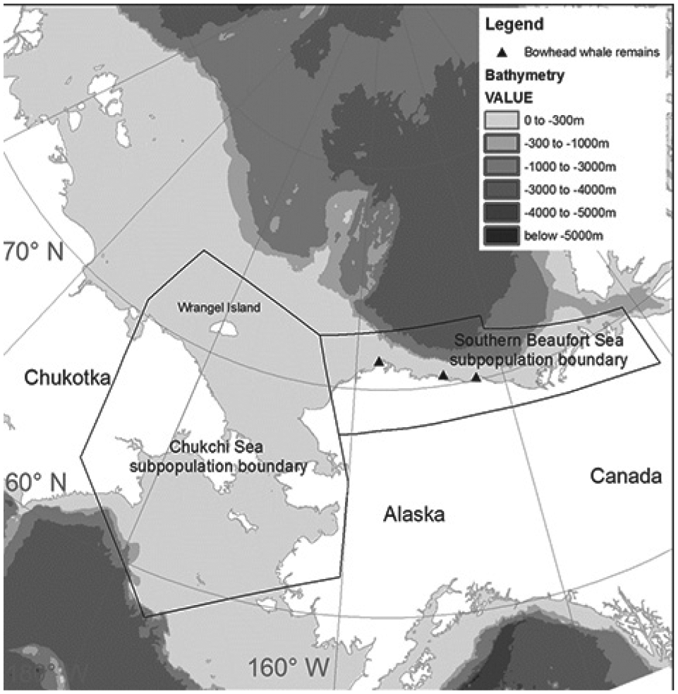
Study area showing the International Union for the Conservation of Nature Polar Bear Specialist Group identified population boundaries for the Southern Beaufort Sea and Chukchi Sea and place names used in the text. Note that bears were assigned to subpopulations in this study based on their locations relative to these identified boundaries.

Activity and Location Data Collection

Activity data were obtained from satellite radio collars (Telonics, Mesa, AZ) using procedures that have been previously described (Rode et al., 2015a). Some bears wore their collars for more than 1 year (n = 39), and some were collared more than once in noncontinuous years (n = 6). We included all activity data regardless of duration of collection and did not censor activity data after capture because activity and movement rates return to normal levels within 2 to 5 days following capture (Rode et al., 2015a).

Collar-housed accelerometers (Telonics) recorded data from 3 axes and internally processed those values before combining them into a single activity value representing the “active” seconds per minute (possible range: 0-60). Then, prior to satellite uplink, the 1-min activity counts were summed into 1 of 4 predeployment set intervals (15 min, 30 min, 2 h, or 3 h) or stored onboard, depending on collar type. The data were then either transmitted via satellite or downloaded from recovered collars. Accelerometer data were quality controlled as previously described by Ware et al. (2017). The radio collars provided global positioning system (GPS) locations every hour with an accuracy of 30 m (D’Eon et al., 2002). Because activity data sampling rates and location data sampling rates did not match (i.e., 15 min, 30 min, 2 h, or 3 h for activity v. 1 h for location), the observed locations and associated accuracies were used to predict polar bear locations for each activity observation using R statistical computing (R Core Team, 2014) package “CRAWL” (Johnson, 2015) as described in Rode et al. (2015b). The CRAWL algorithm accounts for variable location quality and sampling intervals and allows for location estimates to be obtained at user-defined intervals. We predicted locations using the CRAWL method only for data collected <7 days apart; however, CRAWL has been validated to provide accurate locations with data gaps of up to 14 days (Rode et al., 2015b). All activity data were converted from Greenwich Mean Time into local (solar) time using the longitude and latitude associated with each GPS observation.

Activity Analysis

Factors that we expected would affect activity patterns or rhythmicity, including denning, reproductive status, and food availability (described further below), were coded on a monthly scale to match the time scale of the circadian parameters we investigated. Estimates of some circadian parameters, such as rhythm period, require multiple days of consecutive data for reliable estimates. We chose 2-week windows to allow reasonably precise period estimates to be made while also enabling changes over the year to be observed. As seen in Figure 2, results are similar whether a weekly, biweekly, or monthly period analysis is applied. To assess phase of activity, we employed wavelet-based methods that provide time-localized phase marker estimates. We also visually evaluated trends in activity patterns on a 2-week scale to ensure more subtle patterns were not being washed out in the longer sampling intervals (Supplement 1).

Figure 2.

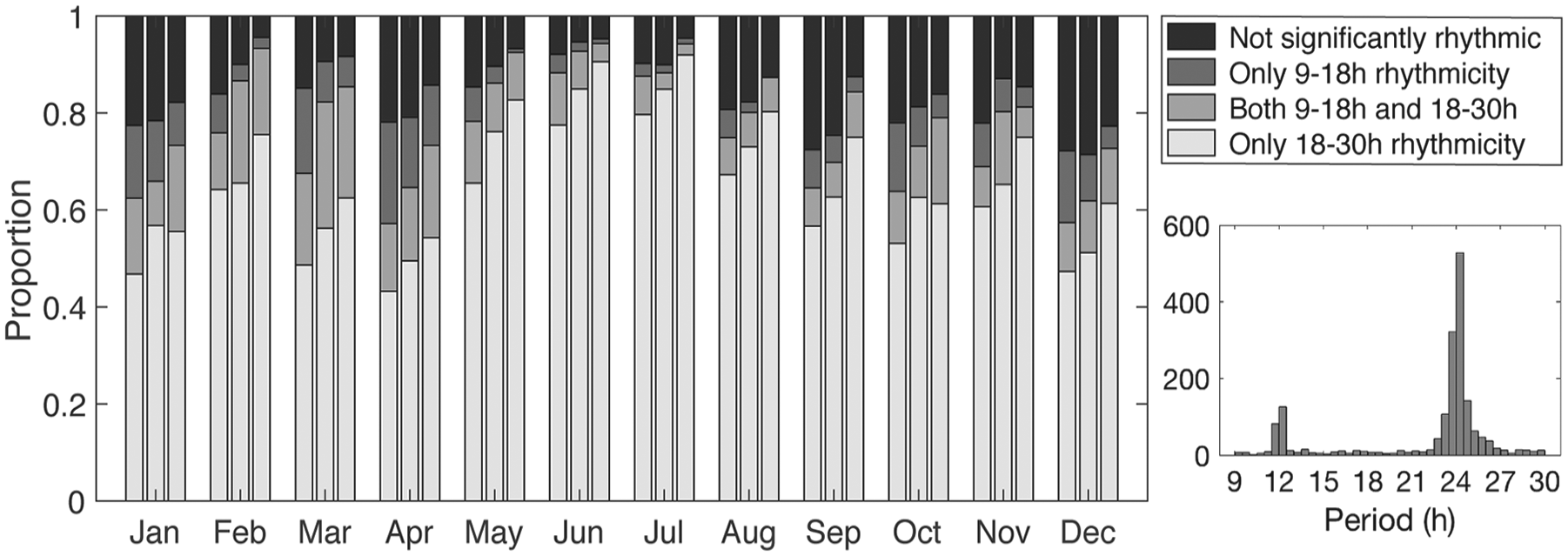
Proportion of rhythmic and arrhythmic animals, in which each group of 3 stacked bars shows results from weekly (left), biweekly (middle), and monthly (right) time windows of the data for the given month. Inset: histogram displaying the distribution of significant periods for the entire data set, with counts of 2-week windows per 30-min period bin.

Denning bears have sharply reduced levels of activity (Messier et al., 1994; Ware et al., 2012), but whether the circadian clock operates in denning polar bears is unknown. Mammals living in nonpolar regions that undergo deep hibernation or daily torpor exhibit a range of circadian characteristics including complete loss of circadian rhythmicity to apparent entrainment to environmental cues and expression of free-running rhythms (Körtner and Geiser, 2000; Heller and Ruby, 2004; Revel et al., 2007; Gür et al., 2009; Healy et al., 2012; Jansen et al., 2016). We identified denning events in the data set using a control chart-based algorithm applied to collar temperature data to identify extended periods of warm temperatures that are indicative of denning events because the insulated snow dens of polar bears result in the collar temperature sensor remaining well above ambient air (Olson, 2017; Rode et al., 2018). If a bear was denning for ≥2 weeks in a month, that month was considered a “denning” month.

To evaluate the potential effect of food availability on circadian rhythmicity, we used recently published seal census data (Reimer et al., 2019; Kelly et al., 2010). Based on these results, we considered April through June to be the peak feeding time of the year for polar bears in the Beaufort and Chukchi Seas, which corresponds with the seal pupping season in early spring. All other months were considered nonpupping times with less food potentially available. We used each bear’s habitat as a further proxy for food availability and any other inherent habitat-influenced impacts on activity patterns (e.g., do bears on land retain rhythmicity as they spend the majority of their day resting versus bears on ice that may be potentially engaging in hunting activities?). Each activity measurement was categorized as occurring on land, on land within 5 km of known whale carcass sites, or on ice using GPS locations from the satellite radio collars as described in Ware et al. (2017). Food availability on land is generally considered to be low, with the exception of the north coast of Alaska, where polar bears have predictable access, most years, to subsistence-harvested bowhead whale (Balaena mysticetus) carcasses at 3 locations (Kaktovik, Cross Island, and Barrow; George et al., 2004; Koski et al., 2005). At these whale carcass sites, activity is predominately nocturnal (Miller et al., 2006), which may be in response to human activity. For determining our month-scaled habitats, we categorized bears whose total number of observations at whale carcass sites comprised 10% or more of their total monthly activity observations as “whale carcass” site for that month. Lastly, ice habitat was considered habitat that was reflective of better food availability than land habitat. When bears occupied both land and ice habitats during a given month, we designated the habitat as “mixed.”

Reproduction and associated hormonal fluctuations are implicated in affecting activity patterns (Goldman, 1999; Kolbe and Squires, 2007; Hatcher et al., 2018). Although previous work suggests that reproductive status affects movement rates and activity levels of polar bears (Messier et al., 1992; Amstrup, 1995; Amstrup et al., 2000), it is not known if activity patterns vary between females based on their reproductive status. To test this, we coded females as having no cubs, cubs of the year, or yearlings/2-year-olds. For females observed with 2-year-olds, we considered those young weaned by April of the year they turned 2 unless the adult female was specifically sighted with her young after that month. In addition, if dependent young were observed with a female, we assumed that those young were alive unless observations suggested otherwise. Following denning, a female’s reproductive status was coded as unknown unless she was sighted with young. If a female did not den, we considered her to be without dependent young.

Characterization of Activity Profiles

Plotting of activity as actograms and period and phase analyses were carried out using custom MATLAB scripts (The MathWorks, Natick, MA), adapted from the code developed for Jansen et al. (2016). The MATLAB scripts are publicly posted (https://osf.io/jqtge/). Because some of the data are unevenly sampled, we used the Lomb-Scargle periodogram to estimate period (Ruf, 1999; Van Dongen et al., 1999). Lomb-Scargle period estimates can remain accurate even when relatively large percentages of data are missing (Ruf, 1999). Periods of nonoverlapping 2-week windows of activity were estimated using plomb in MATLAB with oversampling factor 8 for only those windows with at least half of the time points nonmissing (718 of 2569 were discarded because of insufficient data). The highest peak in power for the 18- to 30-h range was taken as the circadian period estimate, and the highest peak in power for the 9- to 18-h range as the half-day period estimate (indicating activity divided into 2 main bouts each day). Each period estimate was considered significant if greater than the 99th percentile of peak periodogram values of 10,000 shuffled time series (randomization method for significance is used here because these time series do not meet some of the assumptions underlying the theoretical formula). To avoid counting harmonics as significant, only the higher-power peak was counted if the half-day periods equaled half the circadian period. We also discarded peaks for which the dominant peak in power was more than double the smaller peak to avoid counting minor periodicities that did not reflect the main pattern of activity. To avoid skewing our results due to differences in sampling rates and to increase consistency across all bears, we rebinned data sampled at intervals of 15 or 30 min to 2-h time steps to calculate the period and test for significance. This rebinning affected less than 15% of the 2-week windows. The results were minimally changed by this rebinning, with very similar period estimates to those found for the original sampling rates: mean absolute error was 0.06 h between the original and 2-h sampling rate circadian period estimates. The 2-h rebinning provided a significance threshold consistent with the 2-h and 3-h sampled records and rejected only 4% of the 15-min and 30-min sampled 2-week windows considered significant by the original sampling rate.

To estimate times of activity onset, offset, and acrophase, we applied a maximal overlap discrete wavelet transform (DWT), using the wmtsa MATLAB package (https://atmos.uw.edu/~wmtsa/). The la8 filter was used with reflection boundary conditions, and the first and last day of the transformed time series were removed to avoid edge effects. Activity onset and offset times were calculated as the interpolated zero-crossings of the DWT circadian component between peak times and were used to define the daily duration of activity, alpha (α). The peaks of the circadian DWT component (corresponding to a time scale of 16-32 h) were used to estimate the acrophases of activity, using a weighted average between times of onset and offset. If 2 peaks occurred within 18 h with 1 peak less than one-third the height of the other, the smaller peak was rejected. For consistency in the analysis across all bears, as mentioned in the previous paragraph, records with 15- or 30-min sampling intervals were rebinned to 2 h, while records with 2- or 3-h sampling intervals were left as is. For all samples, time was taken as the midpoint of the binning interval. Weekly acrophase estimates were generated by taking the circular mean of peak times within each week of a given record if that week had at least 4 peak times and Rao’s circular spacing test returned p < 0.05, indicating significant grouping of peaks to yield a stable acrophase estimate. This process resulted in 1318 usable bear-week acrophase estimates, the rejection of 981 as having too few peaks (often due to missing data), and 1434 not passing Rao’s test. For comparison, using the 19,742 bear-day acrophases across all records yielded similar results, with circular means of significant weekly acrophases versus all daily acrophases differing on average by 0.40 h across the 52 weeks. See Figures 3 and 4 and Supplemental Figures S1 to S5 for further examples of actograms as well as circular histograms of phase results.

Figure 3.

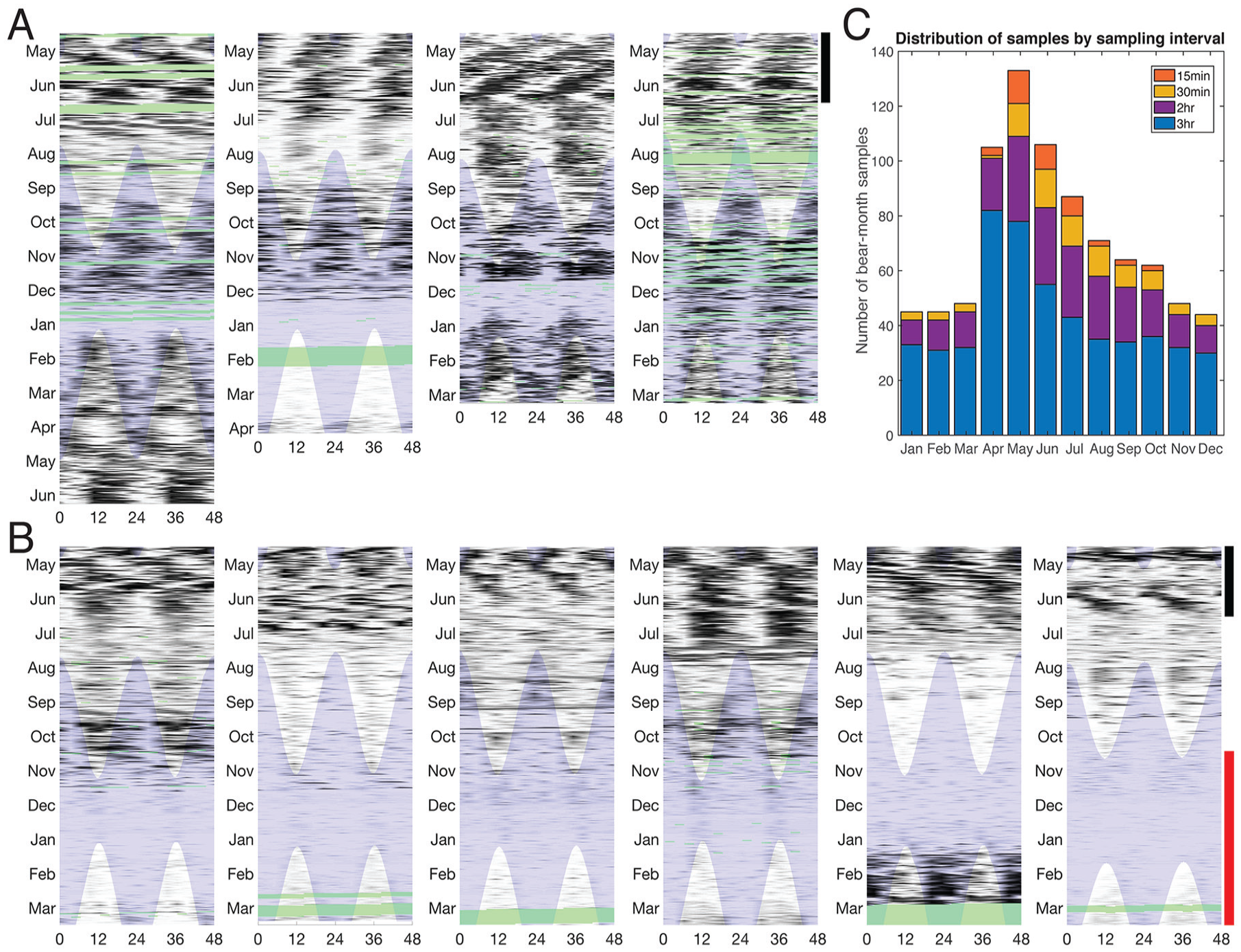
Representative double-plotted actograms illustrating the range of activity patterns of adult female polar bears (local time in hours). (A) Female bears without dependent young and without evidence of denning activity during the months shown. Sampling intervals are either 2 h or 3 h. (B) Denning females (red vertical bar marks range of denning dates) but where cub presence could not be confirmed. Sampling intervals are all 3 h. See the Methods section for denning determination. In both A and B, black vertical bars indicate prime feeding and mating season, light blue shading indicates darkness, and green shading indicates missing data. (C) Distribution of sampling intervals across bear-months for the entire study.

Figure 4.

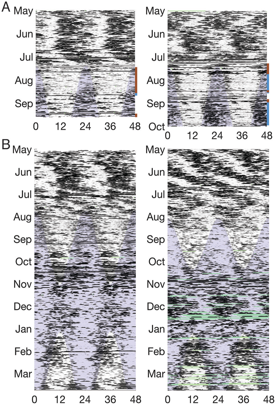
Representative double-plotted actograms of female polar bears with dependent young (local time in hours). (A) Females spending time on ice (no bar), land (brown bar), or within 5 km of a whale carcass (blue bar). (B) Females spending the entirety of the time shown on ice. Sampling interval for all plots is 30 min. Light blue shading indicates darkness, and green shading indicates missing data.

Statistical Analysis

We examined outcomes such as period, rhythmicity, and acrophase using bear-month-year observations (an individual bear’s data for a given month and year) in the statistical analyses. To test the effects of multiple, independent variables on period, we used linear mixed models (SAS Institute, v.9.4 Cary, NC). Photoperiod, calculated from each bear’s location, was included as a continuous covariate. We included feeding period, reproductive status, denning status, and habitat as fixed effect explanatory variables and individual bear as a random effect. A priori interactive effects hypothesized to be important were also included in the models. We used Kenward-Rogers degree-of-freedom estimation and adjusted least-squares means with a Bonferroni p value adjustment to account for unequal denominator degrees of freedom, although linear mixed models are known to be robust against these conditions (Verbeke and Molenberghs, 2009).

We modeled arrhythmia across months as a binomial (“yes” or “no”) variable using a logit link in a generalized linear mixed-model framework including feeding period, reproductive status, denning status, and habitat as fixed effect covariates and individual bear as a random effect. Similar to period analyses, we included photoperiod for each bear-month observation as a continuous covariate. For all of the analyses using the mixed-model approach, we used both ΔAIC (>4) and p value (>0.05) criteria to inform covariate retention in the model in a backward elimination process.

We evaluated differences in the circular variable, acrophase, for feeding period, habitat, reproductive status, and denning in the package “Circular” (Agostinelli and Lund, 2013; R Core Team, 2014) using the Mardia-Watson-Wheeler (MWW) nonparametric test for homogeneity of distributions. We used circular-linear regression to evaluate the effects of photoperiod on acrophases (package “Circular”). Limits to statistical packages prevented multivariate analyses of circular dependent variables. Rao-spacing tests were used to determine whether acrophases were uniformly distributed across the day, and, when applicable (only nonuniform distributions), a mean acrophase was calculated. We considered differences to be statistically significant at p < 0.05.

Results

Collar data from 147 females returned useable records for 122 free-ranging polar bears and yielded a total of 455,710 activity observations and locations. From these data, 862 monthly estimates for period, acrophase, and alpha were computed. No bears spent any time below the Arctic Circle (<66°30′ N) from June to November, and approximately 10% of all observations were above 75° N, with a maximum northerly latitude of 82.5° N. Approximately 50% of the activity recordings above 75° N were in September and October under shortening daylengths around the annual sea ice minimum. Thirteen bears visited 1 of the 3 known whale carcass bone piles (n = 4728 activity observations), with more than 80% of visits occurring between August and October. Denning was confirmed in 29 bears.

Period and Rhythmicity

The majority of bears remained rhythmic throughout the year (Fig. 2), including during periods of constant conditions. Under constant light conditions, 90% of biweekly records exhibited significant circadian (18- to 30-h range) rhythms (24.40 ± 1.39 h, mean ± SD), and only 9% had significant ultradian (9- to 18-h range) rhythms (14.14 ± 2.13h). In contrast, under constant darkness, 59% of biweekly records exhibited circadian periods (23.89 ± 1.72 h) and 21% had ultradian periods (12.12 ± 2.13 h). For bears with no dependent offspring or denning activity, rhythmicity was characterized by high interindividual and intraindividual variability in activity patterns ranging from periods of entrained (τ = 24 h) periodicity, free-running rhythms (i.e., τ ≠ 24 h), arrhythmia, and switches between daytime and nighttime activity (Figs. 3 and 4). Photoperiod had a significant influence on rhythm period, and model fit was best (<AIC) when included as a linear covariate versus nonlinear (quadratic or cubic). Thus, as photoperiod increased, τ increased slightly but significantly (p < 0.001; F1, 646 = 21.23) with peaks during the summer months, the nonprime feeding period (Table 1; Fig. 5). During the prime feeding season (April to June) when seals are pupping, τ was closer to 24 h (τ = 24.06 ± 0.19 h) compared with the nonpupping season (τ = 24.36 ± 0.17 h; p < 0.02, F1, 646 = 5.64). Rhythmicity was characterized by the presence of 2 predominant peaks at 12 and 24 h (Fig. 2, inset). Period was not influenced by other environmental or life history traits (Table 1).

Table 1.

Least squares means (±SE) for period (h) in rhythmic bears and probability of being arrhythmic for fixed-effect explanatory variables included in the multivariate linear and generalized mixed models.

	Rhythmic (Period, h)			Probability of Being Arrhythmic
	LS Means/Estimate	SE	n	LS Means/Estimate	SE	n
Photoperiod	0.04*	0.008	670	0.03	0.03
Feeding period	*			*
Prime feeding	24.06	0.17	265	0.20	0.06	284
Nonprime feeding	24.36	0.19	405	0.10	0.03	434
Habitat
Land	24.34	0.28	26	0.17	0.07	33
Land near whale carcass	24.16	0.38	15	NA	NA	15
Ice	23.98	0.15	530	0.09	0.03	557
Mixed (land and ice)	24.35	0.20	99	0.20	0.07	113
Reproductive status
No young	24.22	0.16	345	0.16	0.03	376
Cubs of the year	24.26	0.22	83	0.16	0.07	89
Yearlings/2-year-olds	24.15	0.18	242	0.11	0.04	253
Denning				*
Yes	24.06	0.28	43	0.24	0.09	43
No	24.36	0.13	579	0.08	0.02	675

p < 0.05 among factors within a group.

Figure 5.

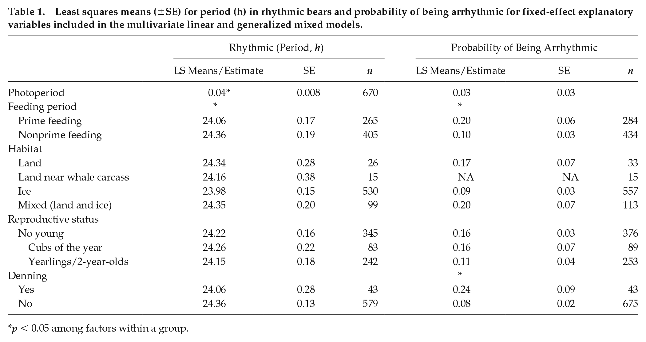
(A) Biweekly periods in the 18- to 30-h range (with Lomb-Scargle peak significant at α = 0.01), showing median (black line), interquartile range (dark gray), and interdecile range (light gray). The sample size for each 2-week window is indicated above the horizontal axis. Tick marks on the horizontal axis indicate the middle of each month. (B) Photoperiod experienced by bears across the year, with median, interquartile range, and interdecile range over bears in each 2-week window. (C) Latitudes of bears across the year, with median, interquartile range, and interdecile range over bears in each 2-week window. (D) Extent of arctic sea ice (area of ocean with at least 15% sea ice), with median, interquartile range, and interdecile range for years 1981 to 2010. Data obtained from National Snow and Ice Data Center (https://nsidc.org/).

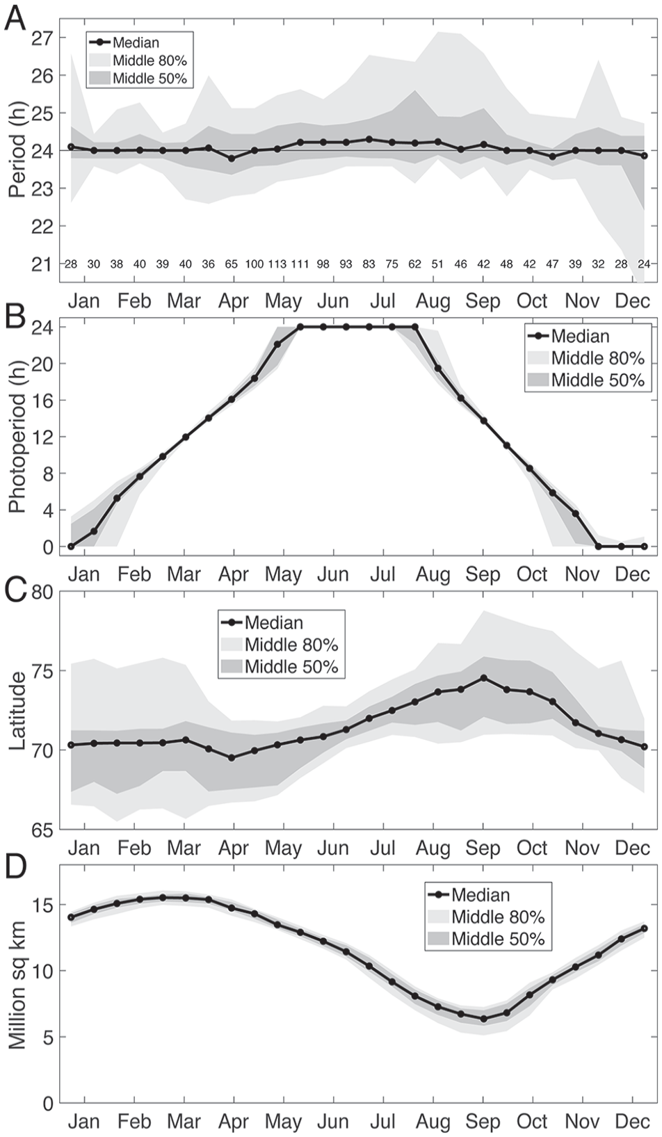
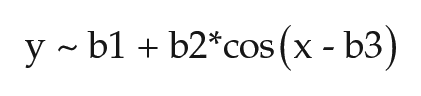
Applying nonlinear regression analysis to describe the annual pattern of polar bear activity rhythms yielded the following model fit:

y ~ b 1 + b 2 * \cos (x - b 3)

where b1 = 24.16 ± 0.04 (mean period in hours), b2 = −0.34 ± 0.06 (maximum change in period across year in hours, above and below mean period), and b3 = 0.51 ± 0.16 (radians; indicates that the longest period occurred during the summer), with p < 0.0001 versus constant model.

Arrhythmia

Arrhythmia was much less likely to be observed (Fig. 2) compared with rhythmic activity patterns in free-ranging polar bears. However, when detected, feeding period, habitat, and denning affected the probability of a bear being arrhythmic (n = 703 bear-months). Polar bears were more likely to be arrhythmic (P_{prime feeding} = 20.3% ± 0.06%) during the prime feeding period compared with the remainder of the year (P_nonpupping = 10.7% ± 0.03%; p = 0.05, F_1,695 = 3.85; Table 1). Denning females had higher (p = 0.02, F_1,695 = 5.52) probabilities of being arrhythmic compared with nondenning females (P_denning = 24.0% ± 0.09% v. P_nondenning = 7.9% ± 0.02%). When bears spent time in both ice and land habitats during a month, the probability of being arrhythmic (P_{ice and land} = 20.5% ± 0.07%) increased (p = 0.04, F_2,695 = 3.36) compared with when they were on ice alone (P_ice = 8.6% ± 0.03%). When bears were on land exclusively, their probability of being arrhythmic was not different than when they were on ice or in a mixture of land and ice. Photoperiod and reproductive status did not affect a bear’s probability of being arrhythmic (Table 1).

Acrophase

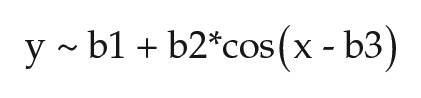
The average time of peak activity (acrophase) remained consistent across much of the year (Fig. 6; Suppl. Fig. S2). However, polar bears occasionally switched temporal patterns from diurnally organized activity to nocturnally organized activity or vice versa when light:dark cycles were present (see example actograms in Figs. 3 and 4). The most striking and consistent “niche switch” occurred during the prime feeding period from April to June, when ringed seals are pupping (Table 2; Fig. 6). Here, monthly acrophases differed significantly from other times of the year (p < 0.001, W = 32.91, MWW test; Table 2), with the net effect being a loss of significant acrophase vector in May (Suppl. Fig. S2). Denning affected acrophase, with denning bears (rhythmic only) having a peak in activity around 14.2 ± 2.7 h, while nondenning bears had a peak of activity at 11.6 ± 6.3 h (p < 0.001; W = 41.88, MWW test; Table 2). There was a slight negative relationship with photoperiod (p < 0.001, circular-linear regression). Acrophase did not differ among habitats (p = 0.10, W = 10.5, MWW test), although variance about the mean for each habitat varied (p < 0.05, χ² = 8.8; Walraff test). Females with cubs of the year (born in January of a given year) had significantly (p < 0.05, W = 10.2, MWW test) shifted acrophases (19.07 ± 2.0 h) compared with independent females (14.13 ± 1.5 h) and females with yearlings or 2-year-olds (13.22 ± 1.5 h; Table 2).

Figure 6.

Bubble plot of weekly acrophases from all bears, where hour 12 is solar noon. The diameter of each blue bubble represents the proportion of samples with acrophase at that hour for that week. The circular mean for each 3-week bin (to ensure sufficient samples) is marked by an orange diamond, whose size is proportional to the synchronization index (a larger diamond indicates more clustered phases). Times of sunrise and sunset at weekly median latitude are indicated by the gray lines. The horizontal axis ticks mark the middle of each month.

Table 2.

Effects of environmental and life history traits on mean monthly acrophase (h ± SE).

Variable	Mean (h)/Estimate	SE (h)
Photoperiod*	−0.009	0.003
Feeding period*
Prime feeding period (n = 275)	13.00	0.45
Nonprime feeding period (n = 379)	14.11	0.27
Habitat
Land (denning excluded; n = 16)	11.46	0.85
Land near whale carcass (12)	15.83	3.46
Ice (n = 482)	14.27	0.29
Mixed (n = 84)	14.84	0.69
Reproductive status*
No cubs (n = 251)	14.1	0.10
Cub of the year (n = 69)	19.1	0.24
Yearling/2-year-old (n = 192)	13.2	0.11
Denning*
Denning (n = 54)	14.2	0.37
Not denning (n = 594)	11.6	0.26

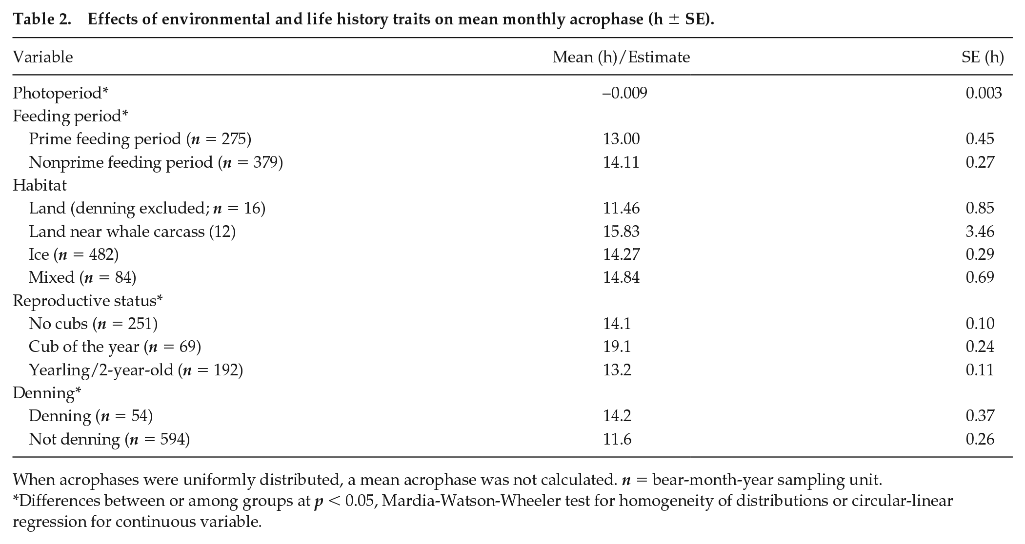
When acrophases were uniformly distributed, a mean acrophase was not calculated. n = bear-month-year sampling unit.

Differences between or among groups at p < 0.05, Mardia-Watson-Wheeler test for homogeneity of distributions or circular-linear regression for continuous variable.

Duration of Activity

Estimates of onsets and offsets (Suppl. Fig. S3) revealed that the monthly average duration of activity α also was relatively constant (range, 10.7 ± 2.7 h to 11.9 ± 2.7 h), with the longest alpha observed in July and the shortest in January. Despite the narrow range, nonlinear regression analysis of biweekly data revealed an annual change in alpha, yielding the following model:

y ~ b 1 + b 2 * \cos (x - b 3)

where b1 = 11.26 ± 0.02 (mean alpha in hours), b2 = −0.53 ± 0.03 (maximum change in alpha across year in hours, above and below the mean alpha value), and b3 = 0.32 ± 0.05 (radians; indicates that the longest alpha occurred during the summer), with p < 0.0001 versus the constant model.

Discussion

The presence of circadian activity rhythms during the polar day and night combined with otherwise stable activity rhythms under rapidly changing day lengths, moving ice, and variable food availability suggests that an endogenous timekeeping system has been conserved in polar bears. Nevertheless, a high degree of behavioral flexibility is observed. This was reflected in extreme variability and a dramatic phase shift, especially when key prey species are available between March and May. Together, these results point to a rapid ability of polar bears to adjust their behavior depending on potential forage availability or life history states. Overall, these results are similar to findings in brown bears (U. arctos), the polar bear’s closest relative (Ware et al., 2012; Jansen et al., 2016), which are also capable of niche switching (Fortin et al., 2013). Polar bears are also similar to other Arctic dwellers, including arctic ground squirrels, bumble bees (Bombus terrestris and Bombus pascuorum), Arctic char (Salvelinus alpinus), red-backed voles (Clethrionomys rutilus), Lapland longspurs (Calcarius lapponicus), and Svalbard reindeer, which retain circadian rhythms even in the absence of light:dark cycles (Swade and Pittendrigh, 1967; Stelzer and Chittka, 2010; Williams et al., 2011; Ashley et al., 2012; Hawley et al., 2017; Williams et al., 2017; Arnold et al., 2018). What makes bears and some Arctic species distinct from those Arctic birds and insects that do not exhibit daily activity rhythms during these periods (Bloch et al., 2013; Steiger et al., 2013; Kobelkova et al., 2015) remains to be determined.

Period length in polar bears increased slightly, but significantly, during the longest days of the Arctic summer. While this might be interpreted to suggest that polar bears are nocturnal based on Aschoff’s rule (i.e., greater light intensity in constant light increases period length in nocturnal animals), light intensity measurements are needed to confirm this. Arguing against this, previous studies showed that daily changes in light intensity in the Arctic are actually quite low during the summer solstice, varying only about 23-fold on a clear day (Swade and Pittendrigh, 1967; Daan and Aschoff, 1975); thus, an effect of light intensity seems improbable. Furthermore, acrophase remained near the middle of the day for most of the year, arguing against a nocturnal niche for polar bears. Another possibility is that the circadian period increased as a result of the lengthening days of summer (i.e., a dose effect), rather than intensity, or was an aftereffect. Support for the former is suggested by the observation that the length of the active period (alpha) also increased slightly with increasing day length, a finding similar to that made in captive brown bears (Ware et al., 2012) and other species (Daan and Aschoff, 1975).

Precisely how polar bears use light cues to entrain locomotor rhythms is unclear. However, given the extreme rates at which day length changes, it could be that bears simply evolved an extremely wide range of entrainment. Alternatively, polar bears may be able to sense changes in light quality (spectral characteristics) via modifications to their intrinsically photosensitive retinal ganglion cells found in mammalian circadian systems (Schmidt et al., 2011; Brown et al., 2012) or other retinal adaptations. Indeed, wavelength and intensity of light can directly influence the SCN (Walmsley et al., 2015) and thereby alter locomotor rhythms of both nocturnal and diurnal species (Nuboer et al., 1983; Pan et al., 2014; Bonmati-Carrion et al., 2017; de Oliveira et al., 2019). Detection of changes in light quality occurring during the day could explain the acrophase and alpha stability observed in polar bears, but actual assessment of retinal anatomy and light quality would be necessary to confirm this. In as far as the authors are aware, only a single published abstract has reported on the retinal anatomy of the polar bear (Peichl et al., 2005). That work revealed that polar bears and brown bears expressed similar retina features such as dichromatic vision and high visual acuity. This is perhaps not surprising as polar bears evolved from brown bears relatively recently and with dietary, rather than visual, adaptations driving this divergence (Liu et al., 2014). Alternatively, bears may be able to use sun orientation to maintain a stable acrophase. Indeed, even at high latitudes, the sun’s azimuth at midday remains stable, while the sun’s altitude changes both seasonally and with latitude (Suppl. Fig. S5). Given that an ice habitat provides little to no obstruction of the sun’s position, this could provide a means whereby bears can organize activity on various time scales. Nevertheless, given the frequent cloud cover and fog in the Arctic, this possibility remains to be confirmed.

The expression of activity rhythms represents a complex interplay between the endogenous clock and environmental cues (Reppert and Weaver, 2002; Kronfeld-Schor and Dayan, 2003). Light is a potent entrainment factor, yet it can also affect behavior through the process of masking, which occurs when environmental stimuli disrupt overt rhythms independently, or downstream, of the central pacemaker itself (Mrosovsky, 1999). In the case of polar bears, our results argue against a strong masking by light/dark on activity rhythms because the activity patterns persist in both constant dark and constant light. However, it is possible that other cues, such as feeding, affected activity patterns via masking or entrainment. Food entrainment can mask the effects of light (Ware et al., 2012; Patton and Mistlberger, 2015), which may be occurring for polar bears, especially in the springtime. Although the distribution of acrophases during spring feeding was highly variable (i.e., some bears were diurnal while others were nocturnal), arrhythmia was also more likely during this time. In particular, from late March to mid-May, bears were more likely to be arrhythmic (19% of 2-week windows) or display ~12-h rhythms (27%), compared with June and July (8% arrhythmic and 7% with ~12-h rhythms). Peak activity was also less likely to occur between solar 0600 h and 1800 h in late March to mid-May (36% of weekly phase estimates) than during June and July (80%). Between May and June, ringed seal pups, not yet fat enough to withstand the cold waters for long, spend significant portions of time on the ice basking (Kelly et al., 2010). Thus, access to seal pups by polar bears is greatest during this period, as reflected in significant hunting (Reimer et al., 2019). Several hunting strategies are used by polar bears, including sitting and waiting or actively searching, and these certainly would have contributed to the variable activity patterns observed. Nevertheless, a tendency to maintain a predawn acrophase during this time of year is evident in the data (Fig. 6). These results suggest that low-light visual acuity in polar bears may be high, and when combined with a highly developed sense of smell (Owen et al., 2015), this could allow for successful predation under low-light conditions.

Flexibility in activity patterns has been demonstrated in many species as a result of anthropogenic influences, predator avoidance, or hunting/foraging (Bejder et al., 2009). For example, the Svalbard reindeer (77°50′–78°20′N), which focus the majority of their annual feeding into the short available summer growing season, showed reduced diel rhythmicity (Arnold et al., 2018). For polar bears at whale carcass sites, previous work showed that feeding occurred mostly at night (Miller et al., 2006). However, in our study, whale carcass visitation and presumed feeding did not affect activity patterns or shift the bears to a nocturnal niche. It should be cautioned that this may be because we determined acrophases using 2-week and month-long windows, rather than daily time scales, leaving open the possibility that polar bears adjust their behavior more frequently. Overall, the high degree of variability among female polar bears living in similar habitats suggests a high degree of behavioral plasticity.

The diverse springtime activity patterns observed could also have been the result of breeding activity, which also occurs at this time of year (Ferguson et al., 2001; Stirling et al., 2016). Field observations of brown bears note high and nearly continuous activity for estrous females being pursued by males (K. Rode, personal communication). Unfortunately, multiple factors prevented us from directly observing and evaluating the effects of estrus and breeding on activity patterns in polar bears. However, observations indicate that female polar bears in estrus are persistently pursued by male followers (K. Rode, personal communication; Stirling et al., 2016), and these behaviors would be consistent with our finding that females in April-June are more likely to become arrhythmic (Table 1). Activity patterns of females denning and producing cubs could also be affected by feeding schedules (Ader and Grota, 1970; Jilge and Hudson, 2001) or activity of offspring. Indeed, denning females were more likely to become arrhythmic, and acrophases were shifted for females with cubs of the year after den emergence. Taken together, these findings suggest that reproductive activity and its associated hormonal fluctuations could have affected activity patterns (Goldman, 1999; Kolbe and Squires, 2007; Hatcher et al., 2018).

Conclusions

Using GPS and accelerometer data, our findings reveal that free-ranging polar bears retain a functioning circadian timing system. This was manifested in the expression of activity rhythms, whose period length was influenced by light exposure. In addition, and despite the rapidly changing day lengths experienced in the Arctic, activity duration and acrophase remained quite stable throughout the year. Nevertheless, high interindividual variability was common, especially during the spring peak feeding season. Overall, the results suggest that a combination of circadian and noncircadian (masking) factors produces the flexible annual activity patterns observed in polar bears. Given their unique ecological niche, it will be important to determine if the behavioral plasticity of polar bears revealed in this study is sufficiently robust to adapt to the loss of sea ice habitat.

Supplemental Material

SuppFigure1 – Supplemental material for The Clock Keeps Ticking: Circadian Rhythms of Free-Ranging Polar Bears

Supplemental material, SuppFigure1 for The Clock Keeps Ticking: Circadian Rhythms of Free-Ranging Polar Bears by Jasmine V. Ware, Karyn D. Rode, Charles T. Robbins, Tanya Leise, Colby R. Weil and Heiko T. Jansen in Journal of Biological Rhythms

Supplemental Material

SuppFigure2_1 – Supplemental material for The Clock Keeps Ticking: Circadian Rhythms of Free-Ranging Polar Bears

Supplemental material, SuppFigure2_1 for The Clock Keeps Ticking: Circadian Rhythms of Free-Ranging Polar Bears by Jasmine V. Ware, Karyn D. Rode, Charles T. Robbins, Tanya Leise, Colby R. Weil and Heiko T. Jansen in Journal of Biological Rhythms

Supplemental Material

SuppFigure3 – Supplemental material for The Clock Keeps Ticking: Circadian Rhythms of Free-Ranging Polar Bears

Supplemental material, SuppFigure3 for The Clock Keeps Ticking: Circadian Rhythms of Free-Ranging Polar Bears by Jasmine V. Ware, Karyn D. Rode, Charles T. Robbins, Tanya Leise, Colby R. Weil and Heiko T. Jansen in Journal of Biological Rhythms

Supplemental Material

SuppFigure4 – Supplemental material for The Clock Keeps Ticking: Circadian Rhythms of Free-Ranging Polar Bears

Supplemental material, SuppFigure4 for The Clock Keeps Ticking: Circadian Rhythms of Free-Ranging Polar Bears by Jasmine V. Ware, Karyn D. Rode, Charles T. Robbins, Tanya Leise, Colby R. Weil and Heiko T. Jansen in Journal of Biological Rhythms

Supplemental Material

SuppFigure5 – Supplemental material for The Clock Keeps Ticking: Circadian Rhythms of Free-Ranging Polar Bears

Supplemental material, SuppFigure5 for The Clock Keeps Ticking: Circadian Rhythms of Free-Ranging Polar Bears by Jasmine V. Ware, Karyn D. Rode, Charles T. Robbins, Tanya Leise, Colby R. Weil and Heiko T. Jansen in Journal of Biological Rhythms

Footnotes

Acknowledgements

The USGS provided funding through the Changing Arctic Ecosystems Initiative and Wildlife Program of the USGS Ecosystems Mission Area. Funding was also provided by the U.S. Fish and Wildlife Service (USFWS). Additional support for data collection was provided by the Detroit Zoological Association, a Coastal Impact Assessment program grant through the State of Alaska, and the National Fish and Wildlife Foundation. Teck Alaska Inc., BP Exploration Alaska, Inc., ARCO Alaska Inc., Conoco-Phillips, Inc., and the Exxon Mobil Production Company provided in-kind support. Any use of trade, product, or firm names is for descriptive purposes only and does not imply endorsement by the U.S. government. The authors express their gratitude to Dave Douglas (USGS) and Ryan Wilson (USFWS) for their assistance with data retrieval and quality-control checks.

Conflict of Interest Statement

The authors have no potential conflicts of interest with respect to the research, authorship, and/or publication of this article.

ORCID iDs

Tanya Leise

Heiko T. Jansen

Data Availability

All data are available at .

Notes

References

Ader

Grota

(1970) Rhythmicity in the maternal behaviour of Rattus norvegicus. Animal Beh 18:144-150.

Agostinelli

Lund

(2013) R package circular: Circular Statistics (version 0.4-3). https://r-forge.rproject.org/projects/circular.

Alerstam

Pettersson

(1991) Orientation along great circles by migrating birds using a sun compass. J Theor Biol 152(2):191-202.

Amstrup

(1995) Movements, distribution, and population dynamics of polar bears in the Beaufort Sea [Ph.D. thesis]. Fairbanks (AK): University of Alaska, Fairbanks.

Amstrup

Durner

Stirling

Lunn

Messier

(2000) Movements and distribution of polar bears in the Beaufort Sea. Can J Zool 78:948-966.

Arnold

Ruf

Loe

Irvine

Ropstad

Veiberg

Albon

(2018) Circadian rhythmicity persists through the polar night and midnight sun in Svalbard reindeer. Sci Rep 8:14466.

Ashley

Schwabl

Goymann

Buck

(2012) Keeping time under the midnight sun: behavioral and plasma melatonin profiles of free-living Lapland longspurs (Calcarius lapponicus) during the arctic summer. J Exp Zool 319:10-22.

Bejder

Samuels

Whitehead

Finn

Allen

(2009) Impact assessment research: use and misuse of habituation, sensitisation and tolerance in describing wildlife responses to anthropogenic stimuli. Mar Eco Prog Ser 395:177-185.

Bentzen

Follmann

Amstrup

York

Wooller

O’Hara

(2007) Variation in winter diet of southern Beaufort Sea polar bears inferred from stable isotope analysis. Can J of Zool 85:596-608.

10.

Bloch

Barnes

Gerkema

Helm

(2013) Animal activity around the clock with no overt circadian rhythms: patterns, mechanisms and adaptive value. Proc R Soc B Biol Sci 280:20130019.

11.

Bonmati-Carrion

Bano-Otalora

Madrid

Rol

(2017) Light color importance for circadian entrainment in a diurnal (Octodon degus) and a nocturnal (Rattus norvegicus) rodent. Sci Rep 7:8846.

12.

Born

Teilmann

Riget

(2002) Haul-out activity of ringed seals (Phoca hispida) determined from satellite telemetry. Mar Mamm Sci 18:167-181.

13.

Bradshaw

Holzapfel

(2007) Evolution of animal photoperiodism. Ann Rev Ecol Evol Sys 38:1-25.

14.

Brown

Tsujimura

S-I

Allen

Wynne

Bedford

Vickery

Vugler

Lucas

(2012) Melanopsin-based brightness discrimination in mice and humans. Curr Biol 22:1134-1141.

15.

Carlens

Lydersen

Krafft

Kovacs

(2006) Spring haul-out behavior of ringed seals (Pusa hispida) in Kongsfjorden, Svalbard. Mar Mamm Sci 22:379-393.

16.

Daan

Aschoff

(1975) Circadian rhythms of locomotor activity in captive birds and mammals: their variations with season and latitude. Oecologia 18:269-316.

17.

Daan

Aschoff

(2001) The entrainment of circadian systems. In: Takahashi

Turek

Moore

, editors. Circadian clocks. Boston: Springer. p. 7-43.

18.

de Oliveira

Scop

Abreu

Sanches

Rossi

Diez-Noguera

Calcagnotto

Hidalgo

(2019) Entraining effects of variations in light spectral composition on the rest-activity rhythm of a nocturnal rodent. Chronobiol Int 36:934-944.

19.

D’Eon

Serrouya

Smith

Kochanny

(2002) GPS radiotelemetry error and bias in mountainous terrain. Wild Soc Bul 30:430-439.

20.

Dunlap

Loros

DeCoursey

(2004) Chronobiology: biological timekeeping. Sunderland (MA): Sinauer Associates.

21.

Durner

Whiteman

Harlow

Amstrup

Regehr

Ben-David

(2011) Consequences of long-distance swimming and travel over deep-water pack ice for a female polar bear during a year of extreme sea ice retreat. Polar Biol 34:975-984.

22.

Fenn

MGP

Macdonald

(1995) Use of middens by red foxes: risk reverses rhythms of rats. J Mamm 76:130-136.

23.

Ferguson

Taylor

Born

Rosing-Asvid

Messier

(2001) Activity and movement patterns of polar bears inhabiting consolidated versus active pack ice. Arctic 54:49-54.

24.

Fortin

Ware

Jansen

Schwartz

Robbins

(2013) Temporal niche switching by grizzly bears but not American black bears in Yellowstone National Park. J Mamm 94:833-844.

25.

George

Zeh

Suydam

Clark

(2004) Abundance and population trend (1978-2001) of western arctic bowhead whales surveyed near Barrow, Alaska. Mar Mamm Sci 20:755-773.

26.

Goldman

(1999) The circadian timing system and reproduction in mammals. Steroids 64:679-685.

27.

Golombek

Rosenstein

(2010) Physiology of circadian entrainment. Physiol Rev 90:1063-1102.

28.

Gür

Refinetti

Gür

(2009) Daily rhythmicity and hibernation in the Anatolian ground squirrel under natural and laboratory conditions. J Comp Physiol B 179:155-64.

29.

Harmsen

Foster

Silver

Ostro

LET

Doncaster

(2011) Jaguar and puma activity patterns in relation to their main prey. Mamm Biol 76:320-324.

30.

Hatcher

Royston

Mahoney

(2018) Modulation of circadian rhythms through estrogen receptor signaling. Eur J Neuro 14184.

31.

Hawley

Rosten

Haugen

Christensen

Lucas

(2017) Freezer on, lights off! Environmental effects on activity rhythms of fish in the Arctic. Biol Let 13:20170575.

32.

Healy

Burdett

Buck

Florant

(2012) Sex differences in torpor patterns during natural hibernation in golden-mantled ground squirrels (Callospermophilus lateralis). J Mamm 93:751-758.

33.

Heller

Ruby

(2004) Sleep and circadian rhythms in mammalian torpor. Ann Rev Physiol 66:275-289.

34.

Heurich

Hilger

Küchenhoff

Andrén

Bufka

Krofel

Mattisson

Odden

Persson

Rauset

(2014) Activity patterns of Eurasian lynx are modulated by light regime and individual traits over a wide latitudinal range. PLoS One 9:e114143.

35.

Hut

Kronfeld-Schor

van der Vinne

De la Iglesia

(2012) In search of a temporal niche: environmental factors. Prog Brain Res 199:281-304.

36.

Jansen

Leise

Stenhouse

Pigeon

Kasworm

Teisberg

Radandt

Dallmann

Brown

Robbins

(2016) The bear circadian clock doesn’t “sleep” during winter dormancy. Front Zool 13:42.

37.

Jilge

Hudson

(2001) Diversity and development of circadian rhythms in the European rabbit. Chronobiol Int 18:1-26.

38.

Johnson

(2015) Package ‘crawl’: fit continuous-time correlated random walk models for animal movement data. https://cran.r-project.org/web/packages/crawl/index.html.

39.

Johnson

Salisbury

Connor

(1967) Ratio of blue to red light: a brief increase following sunset. Science 155:1663-1665.

40.

Jonkel

Kolenosky

Robertson

Russell

(1972) Further notes on polar bear denning habits. Bears: Their Biology and Management 2:142-158.

41.

Kelly

Badajos

Kunnasranta

Moran

Martinez-Bakker

Wartzok

Boveng

(2010) Seasonal home ranges and fidelity to breeding sites among ringed seals. Polar Biol 33:1095-1109.

42.

Kobelkova

Goto

Peyton

Ikeno

Lee

Denlinger

(2015) Continuous activity and no cycling of clock genes in the Antarctic midge during the polar summer. J Insect Physiol 81:90-96.

43.

Kolbe

Squires

(2007) Circadian activity patterns of Canada lynx in western Montana. J Wild Manage 71:1607-1611.

44.

Körtner

Geiser

(2000) The temporal organization of daily torpor and hibernation: circadian and circannual rhythms. Chronobiol Int 17:103-128.

45.

Koski

George

Sheffield

Galginaitis

(2005) Subsistence harvests of bowhead whales (Balaena mysticetus) at Kaktovik, Alaska (1973-2000). J Cetacean Res Manage 7:33-37.

46.

Kronfeld-Schor

Dayan

(2003) Partitioning time as an ecological resource. Ann Rev Ecol Evol System 34:153-181.

47.

Krull

(1976) Zeitgebers for animals in the continuous daylight of high arctic summer. Oecologia 24:149-157.

48.

Kunnasranta

Hyvärinen

Häkkinen

Koskela

(2002) Dive types and circadian behaviour patterns of Saimaa ringed seals (Phoca hispida saimensis) during the open-water season. Acta Theriologica 47:63-72.

49.

Lentfer

Hensel

(1980) Alaskan polar bear denning. Bears: Their Biology and Management 4:101-108.

50.

Liu

Lorenzen

Fumagalli

Harris

Xiong

Zhou

Korneliussen

Somel

Babbitt

, et al. (2014) Population genomics reveal recent speciation and rapid evolutionary adaptation in polar bears. Cell 157:785-794.

51.

Loe

Bonenfant

Mysterud

Severinsen

Øritsland

Langvatn

Stien

Irvine

Stenseth

(2007) Activity pattern of arctic reindeer in a predator-free environment: no need to keep a daily rhythm. Oecologia 152:617-624.

52.

Meng

Q-J

Tyler

Stokkan

K-A

Loudon

(2010) A circadian clock is not required in an arctic mammal. Curr Biol 20:533-537.

53.

Lydersen

(1991) Monitoring ringed seal (Phoca hispida) activity by means of acoustic telemetry. Can J Zool 69:1178-1182.

54.

Merlin

Gegear

Reppert

(2009) Antennal circadian clocks coordinate sun compass orientation in migratory monarch butterflies. Science 325(5948):1700.

55.

Messier

Taylor

Ramsay

(1992) Seasonal activity patterns of female polar bears (Ursus maritimus) in the Canadian Arctic as revealed by satellite telemetry. J Zool 226:219-229.

56.

Messier

Taylor

Ramsay

(1994) Denning ecology of polar bears in the Canadian Arctic Archipelago. J Mamm 75:420-430.

57.

Miller

Proffitt

Schliebe

(2006) Demographics and behavior of polar bears feeding on bowhead whale carcasses at Barter and Cross Islands, Alaska, 2002-2004. Technical report MMS 2006-14 prepared for Minerals Management Service by the U.S. Fish and Wildlife Service, Marine Mammals Management Office, Anchorage, Alaska.

58.

Mrosovsky

(1999) Masking: history, definitions, and measurement. Chronobiol Int 16:415-429.

59.

Munro

RHM

Nielsen

Price

Stenhouse

Boyce

(2006) Seasonal and diel patterns of grizzly bear diet and activity in West Central Alberta. J Mamm 87:1112-1121.

60.

Norton

Gaylord

(2004) Drift velocities of ice floes in Alaska’s northern Chukchi sea flaw zone: determinants of success by spring subsistence whalers in 2000 and 2001. Arctic 57:347-362.

61.

Nuboer

JFW

Vannuys

Vansteenbergen

(1983) Color changes in a light regimen as synchronizers of circadian activity. J Comp Physiol 151:359-366.

62.

Obbard

Thiemann

Peacock

DeBruyn

(2010) 2009 status report on the world’s polar bear subpopulations. Paper presented at: Polar Bears: Proceedings of the 15th Working Meeting of the IUCN/SSC Polar Bear Specialist Group; IUCN; Gland, Switzerland.

63.

Olson

Rode

Eggett

Smith

Wilson

Durner

Fischbach

Atwood

Douglas

(2017) Collar temperature sensor data reveal long-term patterns in southern Beaufort Sea polar bear den distribution on pack ice and land. Mar Ecol Prog Ser 564:211-224.

64.

Owen

Swaisgood

Slocomb

Amstrup

Durner

Simac

Pessier

(2015) An experimental investigation of chemical communication in the polar bear. J Zool 295:36-43.

65.

Pan

Yang

(2014) Artificial polychromatic light affects growth and physiology in chicks. PLoS One 9:e113595.

66.

Patton

Mistlberger

(2015) Circadian adaptations to meal timing: mechanisms. In: Abizaid

Andrews

, editors. Neuroendocrine mechanisms that connect feeding behavior and stress. Lausanne (Switzerland): Frontiers Media SA. p. 26-39.

67.

Peichl

Dubielzig

Kübber-Heiss

Schubert

Ahnelt

(2005) Retinal cone types in brown bears and the polar bear indicate dichromatic color vision. Invest Ophthalmol Vis Sci 46:4539.

68.

Pettersson

Sandberg

Alerstam

(1991) Orientation of robins, Erithacus rubecula, in a vertical magnetic-field. Anim Behav 41:533-536.

69.

Pohl

(1999) Spectral composition of light as a zeitgeber for birds living in the high arctic summer. Physiol Behav 67:327-337.

70.

R Core Team (2014) R: A language and environment for statistical computing. Vienna (Austria): R Foundation for Statistical Computing. https://www.R-project.org.

71.

Reebs

(2002) Plasticity of diel and circadian activity rhythms in fishes. Rev Fish Biol Fisheries 12:349-371.

72.

Reeves

(1998) Distribution, abundance and biology of ringed seals (Phoca hispida): an overview. NAMMCO Scientific Publications 1:9-45.

73.

Reierth

Stokkan

K-A

(1998) Activity rhythm in high Arctic Svalbard ptarmigan (Lagopus mutus hyperboreus). Can J Zool 76:2031-2039.

74.

Reimer

Brown

Beltaos-Kerr

de Vries

(2019) Evidence of intraspecific prey switching: stage-structured predation of polar bears on ringed seals. Oecologia 189:133-148.

75.

Reppert

Weaver

(2002) Coordination of circadian timing in mammals. Nature 418:935-941.

76.

Revel

Herwig

Garidou

M-L

Dardente

Menet

Masson-Pévet

Simonneaux

Saboureau

Pévet

(2007) The circadian clock stops ticking during deep hibernation in the European hamster. Proc Natl Acad Sci USA 104:13816-13820.

77.

Rode

Olson

Eggett

Douglas

Durner

Atwood

Regehr

Wilson

Smith

St. Martin

(2018) Den phenology and reproductive success of polar bears in a changing climate. J Mamm 99:16-26.

78.

Rode

Pagano

Bromaghin

Atwood

Durner

Simac

Amstrup

(2015a) Effects of capturing and collaring on polar bears: findings from long-term research on the southern Beaufort Sea population. Wildl Res 41:311-322.

79.

Rode

Wilson

Regehr

Martin

Douglas

Olson

(2015b) Increased land use by Chukchi Sea polar bears in relation to changing sea ice conditions. PloS One 10:e0142213.

80.

Ruf

(1999) The Lomb-Scargle periodogram in biological rhythm research: analysis of incomplete and unequally spaced time-series. Biol Rhythm Res 30:178-201.

81.

Schmidt

Nakanishi

Izawa

Okamura

Watanabe

Tanaka

Doi

(2008) The reproductive tactics and activity patterns of solitary carnivores: the Iriomote cat. J Ethol 27:165-174.

82.

Schmidt

Chen

S-K

Hattar

(2011) Intrinsically photosensitive retinal ganglion cells: many subtypes, diverse functions. Trends Neuro 34:572-580.

83.

Smith

(1982) Light quality, photoperception, and plant strategy. Annu Rev Plant Phys 33:481-518.

84.

Steiger

Valcu

Spoelstra

Helm

Wikelski

Kempenaers

(2013) When the sun never sets: diverse activity rhythms under continuous daylight in free-living arctic-breeding birds. Proc Biol Sci 280:20131016.

85.

Stelzer

Chittka

(2010) Bumblebee foraging rhythms under the midnight sun measured with radiofrequency identification. BMC Biol 8:93.

86.

Stern

Laidre

(2016) Sea-ice indicators of polar bear habitat. Cryosphere 10:2027-2041.

87.

Stirling

Spencer

Andriashek

(2016) Behavior and activity budgets of wild breeding polar bears (Ursus maritimus). Mar Mamm Sci 32:13-37.

88.

Swade

Pittendrigh

(1967) Circadian locomotor rhythms of rodents in the arctic. Am Naturalist 101:431-466.

89.

Thiemann

Iverson

Stirling

(2008) Polar bear diets and arctic marine food webs: insights from fatty acid analysis. Ecol Mono 78:591-613.

90.

Thompson

Fedak

McConnell

Nicholas

(1989) Seasonal and sex-related variation in the activity patterns of common seals (Phoca vitulina). J Appl Ecol 26:521-535.

91.

Van Dongen

Olofsen

VanHartevelt

Kruyt

(1999) Searching for biological rhythms: peak detection in the periodogram of unequally spaced data. J Biol Rhythms 14:617-620.

92.

van Oort

Tyler

Gerkema

Folkow

Blix

Stokkan

K-A

(2005) Circadian organization in reindeer. Nature 438:1095-1096.

93.

Verbeke

Molenberghs

(2009) Linear mixed models for longitudinal data. New York: Springer Science & Business Media.

94.

Walmsley

Hanna

Mouland

Martial

West

Smedley

Bechtold

Webb

Lucas

Brown

(2015) Colour as a signal for entraining the mammalian circadian clock. Plos Biol 13:e100217.

95.

Ware

Nelson

Robbins

Jansen

(2012) Temporal organization of activity in the brown bear (Ursus arctos): roles of circadian rhythms, light, and food entrainment. Am J Physiol Regul Integr Comp Physiol 303:R890-R902.

96.

Ware

Rode

Bromaghin

Douglas

Wilson

Regehr

Amstrup

Durner

Pagano

Olson

, et al. (2017) Habitat degradation affects the summer activity of polar bears. Oecologia 184:87-99.

97.

Williams

Barnes

Buck

(2011) Daily body temperature rhythms persist under the midnight sun but are absent during hibernation in free-living arctic ground squirrels. Biol Lett 8:31-34.

98.

Williams

Barnes

Buck

(2015) Persistence, entrainment, and function of circadian rhythms in polar vertebrates. Physiology (Bethesda) 30:86-96.

99.

Williams

Barnes

Yan

Buck

(2017) Entraining to the polar day: circadian rhythms in arctic ground squirrels. J Exp Biol 220:3095-3102.

100.

Wilson

Culik

Kosiorek

Adelung

(1998) The over-winter movements of a chinstrap penguin (Pygoscelis antarctica). Polar Rec 34:107-112.

Supplementary Material

Please find the following supplemental material available below.

For Open Access articles published under a Creative Commons License, all supplemental material carries the same license as the article it is associated with.

For non-Open Access articles published, all supplemental material carries a non-exclusive license, and permission requests for re-use of supplemental material or any part of supplemental material shall be sent directly to the copyright owner as specified in the copyright notice associated with the article.

0.00 MB

3.73 MB

0.19 MB

1.21 MB

4.21 MB

0.73 MB