Sage Journals: Discover world-class research

Abstract

An improvement to our current quantitative model of arousal state dynamics is presented that more accurately predicts sleep propensity as measured with sleep dynamics depending on circadian phase and prior wakefulness. A nonlinear relationship between the circadian variables within the dynamic circadian oscillator model is introduced to account for the skewed shape of the circadian rhythm of alertness that peaks just prior to the onset of the biological night (the “wake maintenance zone”) and has a minimum toward the end of the biological night. The revised circadian drive thus provides a strong inhibitory input to the sleep-active neuronal population in the evening, counteracting the excitatory effects of the increased homeostatic sleep drive as originally proposed in the opponent process model of sleep-wake regulation. The revised model successfully predicts the sleep propensity profile as reflected in the dynamics of the total sleep time, sleep onset latency, wake/sleep ratio, and sleep efficiency during a wide range of experimental protocols. Specifically, all of these sleep measures are predicted for forced desynchrony schedules with day lengths ranging from 1.5 to 42.85 h and scheduled time in bed from 0.5 to 14.27 h. The revised model is expected to facilitate more accurate predictions of sleep under normal conditions as well as during circadian misalignment, for example, during shiftwork and jetlag.

Keywords

circadian homeostatic sleep propensity modeling circadian phase wake maintenance zone forced desynchrony

Sleep propensity, defined as the likelihood of falling or remaining asleep at any given moment (Dijk and Czeisler, 1995; Bes et al., 2009), is a fundamental expression of sleep-wake regulation and largely determines the timing and duration of sleep. Sleep propensity, as demonstrated with various sleep-related measures, including sleep onset latency (SOL) and total sleep time (TST), is maximal during the biological night and minimal in the evening just prior to the onset of the biological night. This 2- to 3-h window of reduced sleep propensity ends at the onset of melatonin synthesis under entrained conditions and is known as the wake maintenance zone (WMZ; Lavie, 1986; Dijk and Czeisler, 1995; Dijk et al., 1997; Dijk et al., 1999; Shekleton et al., 2013). This, apparently paradoxical, reduction in the propensity to sleep in the evening is driven by the opposing interaction between the sleep homeostasic and the circadian drives. The wake-promoting circadian signal, controlled by the suprachiasmatic nucleus (SCN) of the hypothalamus, increases throughout the waking day, peaking in the evening, and overrides the increased homeostatic drive for sleep that occurs with increasing time awake, resulting in the WMZ (Borbély et al., 1989). The wake-promoting role of the circadian system is further demonstrated given that SCN lesions lead to loss of the circadian rhythm in sleep and increase the total duration of sleep per day (Edgar et al., 1993). These mechanisms have to be taken into account when one aims to model sleep and alertness dynamics, particularly under conditions of circadian misalignment. In the current study, therefore, we propose an improvement to our earlier arousal state model to enable more accurate prediction of sleep propensity (see, e.g., Postnova et al., 2013).

The relative contributions of circadian and homeostatic processes to sleep propensity are generally studied in forced desynchrony (FD) protocols, where sleep-wake cycles are set at a “day” length, T, that the circadian system cannot entrain to, typically either significantly longer or shorter than 24 h (e.g., Lavie, 1986; Dijk and Czeisler, 1995; Dijk et al., 1997, 1999; Wyatt et al., 1999, 2004; Münch et al., 2005; Buysse et al., 2005; Grady et al., 2010; Zhou et al., 2011). These schedules forcibly desynchronize the sleep-wake and light-dark cycles from the endogenous circadian clock, so that sleep opportunities are scheduled across all circadian phases, thereby enabling examination of the effects of the circadian phase on sleep while holding prior wake duration constant. These studies collectively demonstrate that wakefulness is maximal (or sleep propensity is minimal) around 240 to 270 circadian degrees (where 0/360° is defined at the peak in the blood plasma melatonin rhythm), which corresponds to WMZ appearing at 2000 to 2200 h under entrained conditions, assuming a sleep onset of 0000 h (Dijk et al., 1997). The WMZ is associated with an increase in alertness and performance (Lavie, 1986; Strogatz et al., 1987; Wyatt et al., 2004; Shekleton et al., 2013) and is followed by an abrupt increase in sleep propensity as the circadian drive decreases rapidly, coincident with the beginning of melatonin synthesis signaling the start of the biological night. A high propensity to sleep is sustained throughout the biological night, reaching a maximum at about 345° (0300 h) until decreasing again at ~60° to 90° (0800-1000 h), and decreases gradually through the day until the minimum in the evening.

Existing models that predict sleep propensity either do not directly reproduce the above experimental studies or have not been tested for their ability to do so. The 2-process model used a circadian oscillator that peaked in the subjective evening to successfully predict the overall profile of daytime vigilance (Borbély et al., 1989; Achermann and Borbély, 1994). The model was not tested against data from FD protocols, however. A neuronal-level model of sleep-wake cycles by Rempe et al. (2010) used the skewed sine function from Borbély et al. (1989) as a circadian input that peaked in the evening to simulate the FD data from Dijk and Czeisler (1995) but underestimated the TSTs, with zero sleep predicted between 90° and 200° (with 0° defined as core body temperature [CBT] minimum), corresponding to 1200 to 2000 h under entrained conditions. Finally, the functional model by Bes et al. (2009) reproduced the continuous sleep propensity profile as a function of multiplicatively related circadian and homeostatic processes, whose time course was derived from latency to rapid eye movement sleep and delta power, respectively. By design, this model requires sleep times as an input to predict sleep propensity profile, however, which precludes prediction of sleep times and direct comparison with FD data.

Our previous model of arousal state dynamics combined a physiologically based model of the ascending arousal system with a functional model of the dynamic circadian oscillator. It was calibrated and tested on a number of experimental protocols, including the effect of diurnal preferences on sleep timing, the effects of light on the circadian phase, and spontaneous internal desynchrony (Phillips et al., 2010, 2011; Postnova et al., 2012, 2013, 2014). It failed, however, to reproduce the sleep propensity profile observed during FD protocols, predicting the lowest propensity to sleep in the afternoon around 1500 h, several hours earlier than the experimentally observed WMZ. In this study, therefore, we aimed to improve our model of the arousal state dynamics to enable more accurate prediction of the sleep propensity profile and validate the model against experimental data.

Models and Methods

Our original model of the arousal state dynamics consists of 2 earlier models: a model of the ascending arousal system developed by Phillips and Robinson (2007) and a model of the circadian oscillator by St. Hilaire et al. (2007). It has been described previously elsewhere (Phillips et al., 2011; Postnova et al., 2013; Robinson et al., 2015), but, for completeness, we provide a detailed description in the supplementary online material (SOM). Here we focus only on the improvements of this original model required to account for the sleep propensity profile.

Circadian Process in the Old Model

Originally, the circadian process C driving the sleep-wake switch of the Phillips and Robinson (2007) model was simulated as

C_{o l d} = \frac{X + 1}{2},

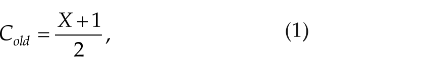
where X (formerly x) is the circadian variable of the St. Hilaire et al. (2007) model, whose dynamics are influenced by both the light-dark cycle and nonphotic inputs. The circadian process $C_{o l d}$ follows the nearly sinusoid shape of the variable X, peaking at ~1530 h under entrained conditions, and is normalized in Eq. (1) to vary approximately between 0 and 1.

Improvement of the Circadian Process: Revised Model

The circadian process as introduced in Eq. (1) results in prediction of the minimum sleep propensity appearing around 1500 h, which does not agree with experimental data showing a WMZ around 2000 to 2200 h (see the Results section for detail). We therefore now revise process C to allow for better agreement with experimental observations. Sleep propensity studies imply that the wake-promoting circadian signal peaks in the evening around WMZ and then decreases rapidly. The minimum of the circadian signal is expected around 0400 to 0600 h. To provide this shape, we introduce a new relationship between the drive C and the variables of the circadian model such that

C = 0.1 C_{o l d} + C_{a d j}^{2},

C_{a d j} = \frac{3.1 X - 2.5 Y + 4.2}{3.7 (X + 2)},

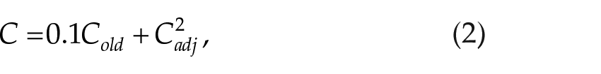
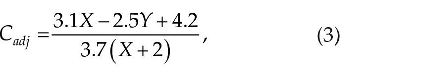
where C_old follows Eq. (1) and X and Y (formerly x_c) are the circadian variables of the St. Hilaire et al. (2007) model. As shown in Figure 1, the new term C_adj causes the shape of the circadian signal to be skewed, with circadian peak appearing at 2220 h and minimum at 0540 h under normal sleep-wake cycles and ambient light conditions. The square of C_adj provides for a rapid decrease of C after its peak to enable the rapid increase of sleep propensity after WMZ. The term C_old maintains a standard sinusoid waveform and allows an increase in circadian amplitude during the growing part of C. 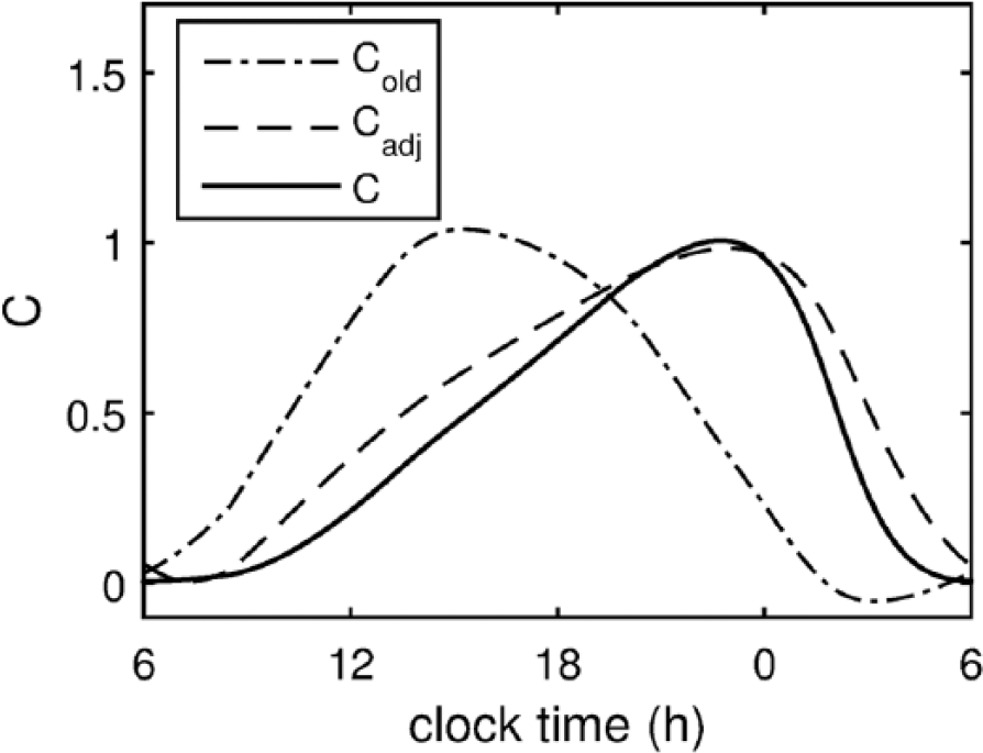The weighted sum of C_old and $C_{a d j}^{2}$ is then the new circadian drive, C, which is shown by a solid line in Figure 1. Note that such a relationship is possible because the circadian variables of the model by St. Hilaire et al. are dimensionless, thus permitting any combination of X and Y to construct drive C. For consistency with prior models, the revised circadian drive C varies approximately between 0 and 1.

Figure 1.

Time course of the revised circadian process C. The revised circadian process shown with a solid line is a weighted sum of the squared adjusted circadian signal C_adj (dashed line) and the circadian process of the previous model version C_old (dashed-dotted line). The dynamics are recorded under ambient light conditions with normal sleep-wake cycles, that is, sleep between 2330 and 0800 h.

Normal Sleep-Wake Cycles

We define the normal sleep dynamics as sleep starting at ~2330 h with a duration of ~8.5 h. We increased the default sleep duration from 8 h in our previous studies to satisfy the experimental findings demonstrating that sleep duration reaches an average asymptote of ~8.5 h (8.12-8.7 h) in young people (Wehr et al., 1993; Van Dongen et al., 2003; Rajaratnam et al., 2004). To achieve these dynamics in ambient light conditions (see below) with our revised circadian drive, we adjust the values of the homeostatic time constant (τ_H), rate of homeostatic growth (v_Hm), and external input to the MA population (A_m). Once adjusted, the parameters are fixed for all simulations.

Ambient Light Profile

Unless otherwise specified, we set ambient light in the model to I = 250 lx between 0800 and 2000 h, I = 40 lx between 2000 and 0800 h if awake, and I = 0 lx during sleep, where light levels are given in photopic lux and a standard white light source (4100K fluorescent lamp) is assumed. The effects of light on the circadian process are realized via the light-dependent dynamics of the St. Hilaire et al. (2007) model, which accounts for the experimentally observed circadian dose response and phase response to light. In simulations, ambient light is used during baseline days before the experimental protocol starts.

Simulated Experimental Protocols

To test the model, we simulate 8 experimental FD protocols with enforced sleep-wake (T) cycles with a duration of T = 1.5 h, T = 3.75 h, T = 20 h, T = 28 h (n = 3), and T = 42.85 h (n = 2; Buysse et al., 2005; Münch et al., 2005; Wyatt et al., 1999; Dijk and Czeisler, 1995; Dijk et al., 1997, 1999; Wyatt et al., 2004; Grady et al., 2010). From the published FD studies available, a sample of those presenting objective sleep data are selected, and only the data from control/young participants are used.

All simulated studies have similar design in that 1) in all experimental cases, the sleep:wake ratio was 1:2, similar to physiological sleep-wake cycles, and 2) lighting during scheduled sleep was 0 lx and during scheduled wakefulness was <15 lux (I = 10 lx in simulations) except for Buysse et al. (2005; T = 3.75 h), where lighting during the scheduled wakefulness was reported to be between 50 and 250 lx depending on the angle of gaze, (I = 100 lx in simulations). The scheduled sleep-wake cycles were repeated between 14 and 40 times, depending on the value of T, to collect sufficient information on sleep dynamics at different circadian phases. In all experiments, participants started the protocol in an entrained and well-rested state by controlling sleep-wake timing and sleep duration prior to laboratory admission and during initial baseline sleep nights in the laboratory.

Circadian Phase Estimation

Circadian phase in the experiments was estimated by 1) the timing of the core body temperature rhythm minimum (CBTmin) when collected under highly controlled conditions (Dijk and Czeisler, 1995; Dijk et al., 1999; Wyatt et al., 1999; Grady et al., 2010) or 2) the timing of the plasma melatonin peak (MELpeak) when measured under highly controlled lighting conditions (Dijk et al., 1997; Wyatt et al., 2004). The timing of the CBTmin and MELpeak in the model are calculated based on the formulas provided in earlier studies (St. Hilaire et al., 2007) and adjusted once to fit baseline data from Dijk and Czeisler (1995) for CBTmin and Dijk et al. (1997) for MELpeak. The values obtained are then used across all other studies, as detailed in the SOM.

In the ultra-short FD protocols (Münch et al., 2005; Buysse et al., 2005), circadian phase was not measured and data were reported against clock time. Clock time was taken as a proxy for circadian time assuming that the participants were entrained when starting the protocol and would not have phase shifted substantially during the short protocols, minimizing potential error. We wish to compare our model to data from a wide range of protocols, and, while it is preferable to have actual circadian phase data, there are no published ultra-short FD studies reporting circadian phase using a reliable marker to our knowledge, and so the above studies are included for completeness.

Parameter Calibration and Fitting

Most of the parameters of the revised model remain the same as in the prior model version, which was calibrated on multiple experimental protocols (Phillips and Robinson, 2007; St. Hilaire et al., 2007; Phillips et al., 2011; Postnova et al., 2012, 2013; Fulcher et al., 2014; Postnova et al., 2014). The shape and strength of the circadian drive, as well as time constants of neuronal populations, are adjusted based on the study by Dijk and Czeisler (1995). Further, adjustments of homeostatic parameters are made to reproduce normal sleep-wake dynamics with the new circadian process. More specifically, we have to 1) increase the value of the circadian coupling v_vc to −0.5 from −5.7 mV (i.e., reduce inhibition of the sleep-active neuronal population) to reproduce the non-100% sleep efficiency during the biological night as observed in experiments (Dijk and Czeisler, 1995); 2) increase time constants of the wake- and sleep-active neuronal populations τ_m and τ_v to 50 from 10 s to allow for longer sleep onset latencies (defined as the time between the end of forced wakefulness and sleep onset time) observed in the data even after extended wake intervals (Dijk and Czeisler, 1995); and 3) adjust the homeostatic time constant τ_H and the level of the baseline sleep drive to the ventrolateral preoptic nucleus (VLPO), A_v, to reproduce normal sleep-wake cycles under ambient light conditions and revised parameter values. All these parameter values are provided in the SOM.

To achieve a better fit to specific experimental data, we allow a change in the model parameter V_WE, which sets the minimum voltage of the wake-active monoaminergic neuronal population (MA) during forced/scheduled wakefulness. A change in V_WE reflects the different levels of neuronal activation, which could depend on individual subjects, activities being performed, and/or the effort that is needed to stay awake during the protocol. To estimate quantitatively the goodness of fit of the model to the data, we use root mean-squared error, which is normalized to allow for easier comparison between studies:

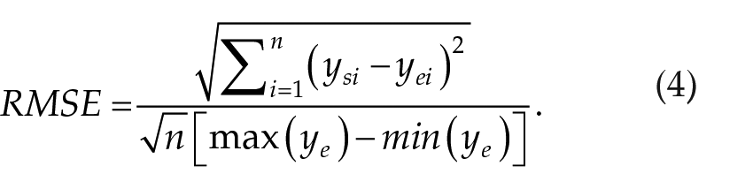
R M S E = \frac{\sqrt{\sum_{i = 1}^{n} {(y_{s i} - y_{e i})}^{2}}}{\sqrt{n} [\max (y_{e}) - m i n (y_{e})]} .

Here, n is the number of data points and y_ei and y_si are the experimental and simulated values at data point i. The best fit by V_WE is found when root mean square error (RMSE) is minimal. Where more than one measure is fitted in the same study, the mean RMSE for these measures is used for fitting the model.

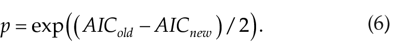
To compare the old and revised model in the view of new parameters being introduced for the circadian process, we calculate the Akaike information criterion (AIC), allowing estimation of a tradeoff between the number of parameters and goodness of fit (Burnham and Anderson, 2003). AIC is calculated for each model and experimental protocol as

A I C = 2 k + n \ln (\sum_{i = 1}^{n} {(y_{s i} - y_{e i})}^{2}),

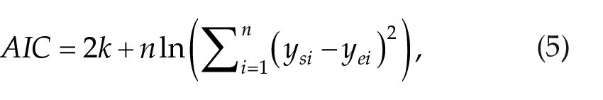
where k is the number of new parameters (k_rev = 4, k_old = 0). The relative probability for the old model to optimize information loss compared with the revised model in each of the experiments is then

p = \exp ((A I C_{o l d} - A I C_{n e w}) / 2) .

Results

To test the revised model for its ability to predict sleep propensity, we examine its dynamics on FD protocols reporting a variety of sleep-related measures with varying durations of the sleep-wake (T) cycles. We separate these studies into 2 categories, those with long (T ≥ 20 h) and short (T = 1.5-3.75 h) T cycles. Figure 2 shows examples of the simulated raster plots for these protocols.

Figure 2.

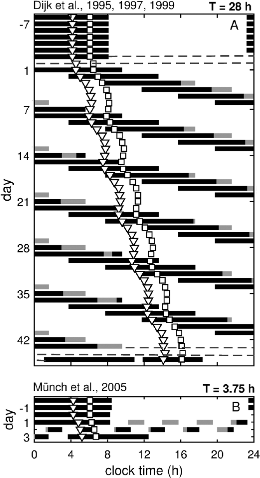
Simulated raster plots for long and short T cycle forced desynchrony protocols. (A) Simulation of the T = 28 h protocol described in Dijk et al. (1995), (1997), and (1999). (B) Simulation of the T = 3.75 h protocol of Münch et al. (2005). Black and gray lines show model predictions for sleep and wake times, respectively, within the scheduled 9.33 h and 1.25 h sleep opportunities. In (A), dashed gray lines before and after the forced desynchrony section show the times of the constant routines. Open triangles (∇) show the predicted position for melatonin peak, and open squares (☐)the core body temperature minimum.

In all FD protocols, T is chosen to be beyond the range of entrainment for the human circadian pacemaker under the light conditions chosen (Klerman et al., 1996). The non–24-h T cycles ensure that sleep is scheduled at different circadian phases, forcibly desynchronizing it from the endogenous circadian clock. The resultant rhythms in sleep quantity and quality highlight the dependence of sleep on the circadian phase at which it is attempted (Figure 2). Furthermore, when the studies employ low lighting conditions, the circadian pacemaker runs close to its endogenous period which, on average, is 24.2 h (Czeisler et al., 1999; Duffy et al., 2011). This is reflected in the simulated dynamics of the circadian markers (CBTmin and MELpeak) shown in Figure 2 demonstrating baseline dynamics and mean daily delay of 0.2 h in agreement with experimental studies (e.g., Dijk and Czeisler, 1995; Dijk et al. 1997).

Model Dynamics under Long T-Cycle FD Protocols

Comparison of the Revised and Old Models: TST and SOL

We now examine predictions of the old and revised models against the data from the 28-h protocol of Dijk and Czeisler (1995) and the results for TST and SOL are shown in Figures 3A and B. The revised model predicts minimum TST = 427 min at 210° (phase relative to CBTmin), baseline TST = 530 min on average during the biological night, and gradual decrease of TST between 0° and 210°, which is in excellent agreement with the experimental data. Predicted dynamics of SOL show similarly good agreement, with SOL peaking at 240° (SOL = 16.57 min) and having a minimum at 0° with SOL = 4.9 min.

Figure 3.

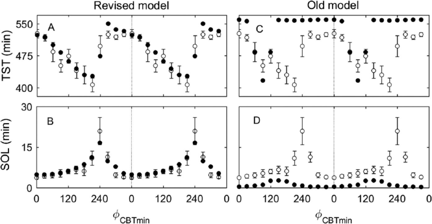
Predictions of sleep dynamics in the revised and old models against experimental observations under the forced desynchrony protocol in Dijk and Czeisler (1995) with T = 28 h. The circadian phase, φ_CBTmin, as calculated relative to the time of the core body temperature minimum, and all data are double plotted. (A) Total sleep time (TST) versus the circadian phase of the middle of the scheduled sleep episode for the revised model. (B) Sleep onset latency (SOL) in a scheduled time-in-bed episode versus the circadian phase of the episode start in the revised model. (C) TST prediction by the old model and (D) SOL prediction by the old model. In all panels, data are averaged across 30° circadian bins and plotted in the middle of the bin. Model predictions are shown with filled circles (•) and experimental data with open circles (⚬) with error bars as reported in Dijk and Czeisler (1995).

On the contrary, predictions from the old model do not agree with the data, as demonstrated in Figures 3C and D. A minimum TST = 417 min is predicted at 90° instead of 210°, and TST = 560 min is predicted at most other circadian phases, which occupies the entire allowed time in bed. SOL in the old model is predicted to be much shorter than in the experiment with a peak of 2.6 min at 120° to 180° and SOL = 0 min at all other phases.

Quantitative comparison of the revised and old model predictions on the protocol of Dijk and Czeisler (1995) is shown in Table 1 using RMSE (see the Methods section). The best fits by the parameter V_WE are found for both models when minimum RMSE was achieved at varying V_WE. The revised model demonstrates up to 4.36 times lower RMSE than the old model. Similarly, we compare quantitative agreement between the model predictions and the data under all other protocols considered, and the revised model shows better agreement with the data in every case, as detailed in Table 1 and below.

Table 1.

Comparison of the best fits to data in the revised and old models. The best fit by V_WE is defined when the minimum root mean square error (RMSE) is achieved for the specific protocol. The default V_WE is obtained as a best fit across all protocols. Data are reported for each of the model versions as well as the degree of improvement as a ratio of best RMSE in the old model version to that of the revised model. Asterisks (*) indicate RMSE calculated for sleep opportunities starting from the fifth data point in Münch et al. (2005) and from the eighth data point in Buysse et al. (2005).

Experiment	Revised Model
	Best Fit		Default		Old Model		Improvement
	V _WE , mV	RMSE	V _WE , mV	RMSE	V _WE , mV	RMSE	Best Fit	Default
Wyatt et al. (2004) SR, T = 42.85 h	0.29	0.193	0.07	0.48	1.85	0.768	3.98	1.6
Grady et al. (2010) SR, T = 42.85 h	0.22	0.153	0.07	0.238	1.89	0.555	3.63	2.33
Dijk et al. (1995) TST, T = 28 h	−0.01	0.140 min⁻¹	0.07	0.181 min⁻¹	1.82	0.611 min⁻¹	4.36	3.38
Dijk et al. (1995) SOL, T = 28 h	−0.01	0.108 min⁻¹	0.07	0.108 min⁻¹	1.82	0.460 min⁻¹	4.26	4.26
Dijk et al. (1997) WR, T = 28 h	0.04	0.145	0.07	0.154	1.75	0.460	3.17	2.99
Dijk et al. (1999) SE, T = 28 h	−0.06	0.104	0.07	0.249	1.65	0.600	5.77	2.4
Wyatt et al. (1999) SE, T = 20 h	−0.23	0.439	0.07	0.670	1.82	0.691	1.57	1.03
Münch et al. (2005) TST, T = 3.75 h	0.33	0.500 min⁻¹ *0.085 min⁻¹	0.07	0.584 min⁻¹ *0.41 min⁻¹	1.23	0.673 min⁻¹ *0.580 min⁻¹	1.34 *6.82	1.15 *1.41
Buysse et al. (2005) TST, T = 1.5 h	0.34	0.210 min⁻¹ *0.125 min⁻¹	0.07	0.287 min⁻¹ *0.3 min⁻¹	2.11	0.473 min⁻¹ *0.624 min⁻¹	2.25 *4.99	1.64 *2.08
Buysse et al. (2005) SOL, T = 1.5 h	0.34	0.255 min⁻¹ *0.160 min⁻¹	0.07	0.348 min⁻¹ *0.353 min⁻¹	2.11	0.515 min⁻¹ *0.630 min⁻¹	2.02 *3.94	1.48 *1.78

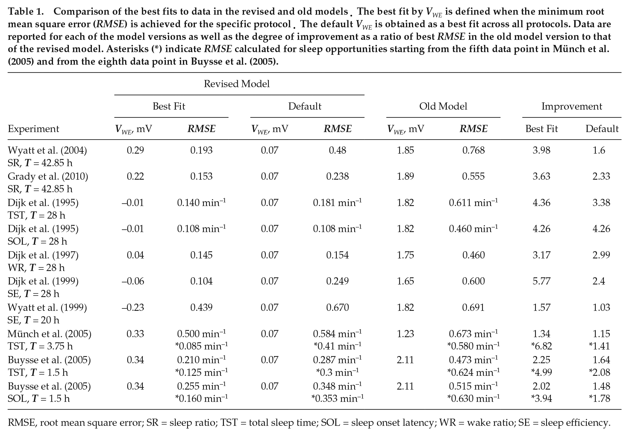
RMSE, root mean square error; SR = sleep ratio; TST = total sleep time; SOL = sleep onset latency; WR = wake ratio; SE = sleep efficiency.

Dynamics of the Revised Model

We further compare the revised model predictions with data from the remaining long T-cycle protocols as summarized in Figure 4.

Figure 4.

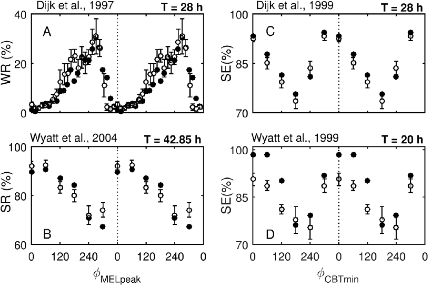
Predictions of sleep propensity measures against the circadian phase under forced desynchrony protocols (T = 20, 28, and 42.85 h). (A) Wake ratio (WR) in the scheduled sleep episodes under the protocol of Dijk et al. (1997) with T = 28 h. (B) Sleep ratio (SR) in the scheduled sleep episodes under the protocol of Wyatt et al. (2004) with T = 42.85 h. For both (A) and (B), the data are plotted against circadian phase relative to the plasma melatonin rhythm (φ_MELpeak, melatonin peak = 0°/360°). Each 30-s epoch during time in bed was defined either as sleep or wake, assigned a circadian phase, and accordingly binned in 15° (A) and 60° (B) bins. WR (SR) was calculated as a percentage of the epochs being in the wake (sleep) state to the total number of the epochs in the given bin. (C) Sleep efficiency (SE) under the protocol of Dijk et al. (1999) with T = 28 h. (D) SE under the protocol of Wyatt et al. (1999) with T = 20 h. The data are plotted against the circadian phase relative to the core body temperature minimum (φ_CBTmin, CBTmin = 0°). SE was calculated as a percentage of time in bed; 9.33 h in (C) and 6.66 h in (D), spent asleep relative to the circadian phase of the middle of the scheduled time in bed. The data are averaged across 60° bins. In all panels, data are plotted in the middle of the bin and are double plotted. Model predictions are shown with filled circles (•) and experimental data with open circles (⚬) with error bars.

Wake and Sleep Ratio

The wake ratio (WR) and sleep ratio (SR) represent the percentage of time within a given circadian phase bin spent in a wake or sleep state, respectively. Figures 4A and B show the model prediction of the WR under the Dijk et al. (1997; T = 28 h) and SR under the Wyatt et al. (2004; T = 20 h) protocols, both of which show excellent agreement with the experimental data.

The model predicts maximum WR at the same circadian phase as observed in the data, that is, at 270° relative to the melatonin peak, which corresponds to the maximum WR at 2200 h in entrained conditions for a person who normally sleeps between 2330 and 0800 h. The WR peak is followed by a rapid decrease both in the data and the model, which then changes to gradual increase between 75° and 270°. The SR profile in Figure 4B qualitatively mirrors that of the WR, but the minimum of SR is predicted at 300° instead of 270° due to the larger bin size (60° vs. 15°) chosen for averaging in the study by Wyatt et al. (2004). We also simulate the study by Grady et al. (2010), which uses a protocol identical to that of Wyatt et al. (2004). Quantitative comparison between the predictions and the experimental data for this study is shown in Table 1 but not illustrated in a figure to avoid redundancy. For all studies above, the RMSE values corresponding to the best fit by V_WE and comparison with the old model are also shown in Table 1.

Both WR and SR profiles are strongly determined by the shape of the circadian signal, which peaks at 2220 h, and the circadian amplitude, v_vc, which allows the nonzero WR (and SR <100%) during biological night. At the best fit by V_WE, the model appears to slightly underestimate WR (and overestimate SR) between 120° and 240°. This may indicate that the circadian amplitude should be higher in this phase interval without changes in others, but this is not easily achieved when the process C is constructed from the circadian variables of the oscillator model.

Sleep Efficiency

Predictions for sleep efficiency compared with the experimental data under FD protocols with T = 28 h (Dijk et al., 1999) and T = 20 h (Wyatt et al., 1999) are shown in Figures 4C and D, respectively. The data are plotted against the circadian phase relative to CBTmin. Note that sleep efficiency differs from SR in that it measures the percentage of time spent asleep within the entire scheduled time in bed (9.33 h in Fig. 4C and 6.66 h in Fig. 4D) relative to the circadian phase of the middle of the scheduled sleep episode instead of calculating the ratio of sleep within a circadian bin.

Under both protocols, the model predicts minimum sleep efficiency at 180°, which corresponds to 1800 h under entrained conditions (CBTmin was reported at 0600 h by Dijk et al., 1999). Under entrained conditions, this means that on average, minimum sleep efficiency would be observed when sleep is scheduled to start between 1120 and 1520 h for T = 28 h and between 1240 and 1640 for T = 20 h. Interestingly, this prediction fits perfectly the data from Dijk et al. (1999), whereas a later minimum, at 240°, is observed in the experimental data on the 20-h protocol. This difference could be attributed to individual variability and a low number of subjects in both studies, but it is also possible that shorter than 24-h sleep-wake cycles produce changes in the circadian process that result in the change of the sleep propensity profile, which are not accounted for in the model. More data from 20-h protocols, however, would be needed to test this.

Model Dynamics under Short T-Cycle FD Protocols

To account for a broad range of sleep propensity data, we test the model dynamics on short FD protocols. In this case, multiple sleep-wake cycles are scheduled within one circadian cycle, with TST and SOL reflecting the sleep propensity profile. The studies included here are those by Münch et al. (2005) with T = 3.75 h and Buysse et al. (2005) with T = 1.5 h.

Figure 5 shows simulations for TST and SOL under the short FD protocols. For both studies, the model shows excellent agreement with data but only starting from the biological evening on the first protocol day (i.e., from about 2200 h). After the first protocol day, high TST is predicted for both studies between 0130 and 1630 h, with a maximum reaching 67.5 min out of 75 min time in bed in Figure 5A and 24 min out of 30 min time in bed in Figure 5B. This high TST observed during early biological day appears due to sleep disturbance introduced by the protocol during the prior biological night in combination with the yet low circadian drive. The minimum TST (after the first protocol day) in both protocols is predicted for sleep episodes scheduled around 2100 h, coincident with the WMZ (Fig. 5). The SOL prediction and experimental data in Figure 5C mirror that of the TST data in Figure 5B, indicating that most of the wake appears in the beginning of the scheduled time in bed.

Figure 5.

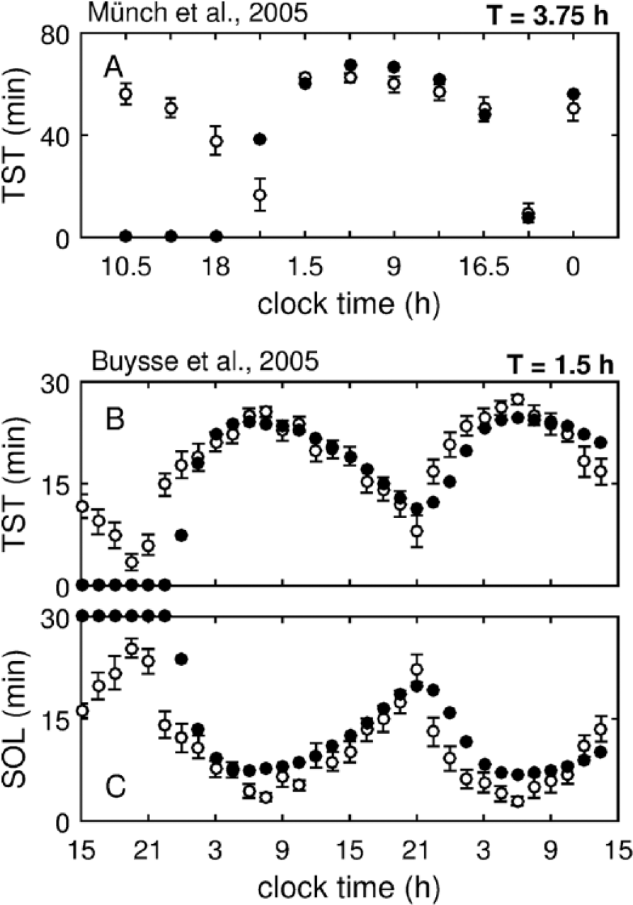
Predictions of sleep propensity measures under short forced desynchrony protocols. (A) Total sleep time (TST) per scheduled time in bed against clock time of the scheduled sleep episode under the protocol of Münch et al. (2005) with T = 3.75 h. (B) TST and (C) sleep onset latency against the clock time of the start of sleep episodes under the protocol of Buysse et al. (2005) with T = 1.5 h. In all cases, experimental data from young subject groups are shown. Model predictions are shown with filled circles (•) and experimental data with open circles (⚬) and error bars.

The model does not agree with the data for the first ~10 h of either protocol. The model predicts no sleep, given that the ultra-short sleep-wake schedules start after a week of controlled sleep at home and one to two 8-h baseline nights in a laboratory. In the data, however, high TST is present during the naps directly following the baseline sleep. These data likely indicate that the participants retain some sleep debt at the start of the study and are not sleep satiated (Wehr et al. 1993; Van Dongen et al. 2003; Rajaratnam et al. 2004). Another explanation would be that even at zero sleep debt, sleep can be initiated if a person is exposed to the right environmental conditions, for example, darkness and quiet. The latter is in agreement with the somnificity concept, which states that sleep propensity is affected by environmental conditions, posture, and activity (Johns, 2002) but is not yet accounted for in the model.

Predictions

The values for the parameter V_WE are constrained to the range between −0.23 and 0.34 mV by the best-fit values obtained for the above simulations. Remarkably, the parameter values are clustered according to the length of the T cycle with larger T associated with larger V_WE for long protocols: V_WE = −0.23 mV for T = 20 h, V_WE = {–0.06; −0.01; 0.04} mV for T = 28 h, and V_WE = {0.22; 0.29} mV for T = 42.85 h. Ultrashort protocols, however, are associated with the largest best fit values of V_WE = {0.33; 0.34} mV. This may indicate an increase of V_WE with time awake on the long protocols, which may be considered in future studies. The high V_WE values on the ultra-short protocols may be associated with sleep inertia, which has a strong influence over the short wake episodes compared with protocols with large T.

All V_WE values from the constrained range can be used in future predictions to provide qualitative predictions of sleep propensity. To determine the best overall value of V_WE, however, we find V_WE leading to the lowest mean RMSE across all studies. This value is V_WE = 0.07 mV, and the corresponding RMSE values for each study are shown in Table 1. As expected, the agreement is much better than for the best fits of the old model but slightly worse than for individual fits to each study in the revised model. The corresponding figures of simulations obtained with V_WE = 0.07 mV are shown in the SOM (Suppl. Figs. S1 and S2). As seen from Table 1, predictions at this new default value of V_WE are better for T = 28 h protocols, which is explained by the higher number of 28 h protocols in the data set compared with other T cycles.

Finally, we compare the revised and old models using AIC to make sure that addition of the new parameters adjusting the shape of the circadian process in Eqs. (2) and (3) does not introduce overfitting. We find that the relative probability for the old model to optimize information loss compared with the revised model is on the order of 10^–6 in 7 of 8 experiments (see Eq. [6] for calculation). This clearly confirms better predictive power of the revised model.

Discussion

We have developed a model of arousal state dynamics that predicts the sleep propensity profile depending on the circadian phase at which sleep is attempted. The model was tested against the data from a wide range of FD protocols with day lengths ranging from 1.5 to 42.85 h to ensure that the interaction between the circadian and homeostatic processes was incorporated correctly. The model agrees exceptionally well with the experimental data and makes correct predictions for SOL, TST, sleep efficiency, and wake/sleep ratio at different circadian phases. To our knowledge, no other model of sleep propensity reproduces such a wide range of experimental data. The revised model should thus allow for better predictions of sleep times and therefore alertness profiles during circadian misalignment, real-world examples of which will be considered in future studies include shiftwork, jet lag, and other circadian sleep-wake rhythm disorders.

The revised model is an improvement of our earlier model (Phillips et al., 2010, 2011; Postnova et al., 2012, 2013 2014) and provides much more accurate fits to the data, as detailed in Table 1. To achieve this improvement, the circadian input in the model was modified to 1) peak in the evening (≡2220 h under entrained conditions), where it counteracts the increased homeostatic drive to sleep, and 2) decrease rapidly after the peak to allow for the steep change in sleep propensity observed experimentally at melatonin onset (Dijk and Czeisler, 1995; Dijk et al., 1997). Such model structure is in line with the opponent-process concept, postulating that the circadian process has an active wake-promoting role during daytime (Borbély et al., 1989; Edgar et al., 1993; Dijk and Czeisler, 1995). A simulated skewed time profile of the circadian drive was originally introduced in several modifications of the original 2-process model using a sum of sine functions (Borbély et al., 1989; Achermann and Borbély, 1994). These studies, together with the present one, support the notion that such a shape of the circadian input, with a peak in the evening, is essential to properly reproduce sleep propensity as well as alertness. The advantage of the present study, however, is that we maintain the link to the dynamic circadian oscillator, allowing for the effects of light on the circadian oscillator, which is essential in future research (e.g., on shiftwork).

The refined time course of the circadian process is achieved by introducing a function of the variables X and Y of the circadian model, as shown in Eqs (2) and (3). This is a simple way to combine the dynamic circadian model with the model of the ascending arousal system without introducing new variables. Mathematically, similar shapes can also be achieved with other transformations involving X and Y allowing for correct predictions of sleep propensity. The key is to maintain the timings of the peak and trough as well as the gradient of change.

To achieve good quantitative agreement with the data in the revised model, we had to 1) reduce the strength of circadian inhibition of the VLPO (v_vc) and 2) increase the time constants of MA and VLPO (τ_m, τ_v). The reduction of the circadian inhibition allowed us to account for the correct sleep durations during biological night, while the increase of the time constants allowed for a better quantitative fit for SOL. The increase of time constants slows the transitions between sleep and wake. As a result, we not only increased baseline sleep latency but also introduced a longer transition to full wakefulness when the model is woken up by external stimuli before the physiologically predicted wake-up time (e.g., by an alarm clock).

Surprisingly, to fit the model to each individual study, we needed to change only one model parameter: the minimum MA voltage during forced wakefulness, V_WE. This change reflects different levels of MA activation (e.g., depending on activities being performed and/or the effort that is needed to stay awake during the protocol). Physiologically, there is more than one parameter different between the groups of subjects in each of the considered studies, especially given the small n in each of them. However, use of V_WE allows us to minimize the number of changes. This parameter affects the rate of homeostatic accumulation during forced wakefulness, via the dependence of H on Q_m (see Eq. [S4] in SOM), thereby influencing sleep drive. The main constrain on this parameter is that it has to be above the sleep threshold set to −2 mV and below physiologically justified maximum levels of activity (i.e., 5 mV, as suggested by Phillips and Robinson, 2007). As shown in Table 1, in the studies shown here, the best fit to data is achieved at V_WE between −0.23 mV and 0.34 mV, which satisfies both conditions and further constrains the parameter. The range of V_WE in the revised model is thus 0.57 mV, which is smaller than in the old (0.88 mV), showing that V_WE is better constrained in the revised model.

We have also calculated the best overall fit across studies at V_WE = 0.07 mV, which is set to be a new default value for this parameter and is suggested as the best choice for prospective predictions under FD. Note, however, that observed differences in the best fit V_WE are associated with differences in the subject groups and study conditions, so no single value of V_WE would be able to match all studies equally well.

The outcomes of most of our earlier studies are not affected by the new modification, because they modeled sleep at a fixed phase angle and therefore were not concerned with dependence of sleep duration on the circadian phase (for summary, see Robinson et al., 2015). The modeling studies that may be affected are those concerned with circadian misalignment, where sleep would be attempted at a different circadian phase (Postnova et al., 2012, 2013, 2014). To test this assumption, we repeated the study in Postnova et al. (2013), which compared the effects of bright versus normal light during night shifts on the circadian phase and sleep duration. The outcomes for the revised model showed better quantitative agreement with the experiment than the previous version of the model, whereas qualitatively, the dynamics are the same. It is thus expected that the revised model will more accurately predict sleep measures during shiftwork, which will be examined in detail in future.

Footnotes

Acknowledgements

This research was supported by Australian Government via Cooperative Research Centre for Alertness, Safety and Productivity and the Australian Laureate Fellowship Program (ARC Centre Grant FL140100025).

Notes

References

Achermann

Borbély

(1994) Simulation of daytime vigilance by the additive interaction of a homeostatic and a circadian process. Biol Cybern 71:115-121.

Bes

Jobert

Schulz

(2009) Modeling napping, post-lunch dip, and other variations in human sleep propensity. Sleep 32:392-398.

Borbély

Achermann

Trachsel

Tobler

(1989) Sleep initiation and initial sleep intensity: interactions of homeostatic and circadian mechanisms. J Biol Rhythms 4:149-160.

Burnham

Anderson

(2003) Model Selection and Multimodel Inference: A Practical Information-Theoretic Approach. New York: Springer Science & Business Media.

Buysse

Monk

Carrier

Begley

(2005) Circadian patterns of sleep, sleepiness, and performance in older and younger adults. Sleep 28:1365-1376.

Czeisler

Duffy

Shanahan

Brown

Mitchell

Rimmer

Ronda

Silva

Allan

Emens

. (1999) Stability, precision, and near-24-hour period of the human circadian pacemaker. Science 284:2177-2181.

Dijk

Czeisler

(1995) Contribution of the circadian pacemaker and the sleep homeostat to sleep propensity, sleep structure, electroencephalographic slow waves, and sleep spindle activity in humans. J Neurosci 15:3526-3538.

Dijk

Duffy

Riel

Shanahan

Czeisler

(1999) Ageing and the circadian and homeostatic regulation of human sleep during forced desynchrony of rest, melatonin and temperature rhythms. J Physiol 516(2):611-627.

Dijk

Shanahan

Duffy

Ronda

Czeisler

(1997) Variation of electroencephalographic activity during non-rapid eye movement and rapid eye movement sleep with phase of circadian melatonin rhythm in humans. J Physiol 505(3):851-858.

10.

Duffy

Cain

Chang

Phillips

AJK

Münch

Gronfier

Wyatt

Dijk

Wright

Czeisler

(2011) Sex difference in the near-24-hour intrinsic period of the human circadian timing system. Proc Natl Acad Sci USA 108 Suppl:15602-15608.

11.

Edgar

Dement

Fuller

(1993) Effect of SCN lesions on sleep in squirrel monkeys: evidence for opponent processes in sleep-wake regulation. J Neurosci 13:1065-1079.

12.

Fulcher

Phillips

AJK

Postnova

Robinson

(2014) A physiologically based model of orexinergic stabilization of sleep and wake. PLoS One 9:e91982.

13.

Grady

Aeschbach

Wright

Czeisler

(2010) Effect of modafinil on impairments in neurobehavioral performance and learning associated with extended wakefulness and circadian misalignment. Neuropsychopharmacology 35:1910-1920.

14.

Johns

(2002) Sleep propensity varies with behaviour and the situation in which it is measured: the concept of somnificity. J Sleep Res 11:61-67.

15.

Klerman

Dijk

Kronauer

Czeisler

(1996) Simulations of light effects on the human circadian pacemaker: implications for assessment of intrinsic period. Am J Physiol 270:R271-R282.

16.

Lavie

(1986) Ultrashort sleep-waking schedule. III. “Gates” and “Forbidden zones” for sleep. Electroencephalogr Clin Neurophysiol 63:414-425.

17.

Münch

Knoblauch

Blatter

Schröder

Schnitzler

Kräuchi

Wirz-Justice

Cajochen

(2005) Age-related attenuation of the evening circadian arousal signal in humans. Neurobiol Aging 26:1307-1319.

18.

Phillips

AJK

Chen

Robinson

(2010) Probing the mechanisms of chronotype using quantitative modeling. J Biol Rhythms 25:217-227.

19.

Phillips

AJK

Czeisler

Klerman

(2011) Revisiting spontaneous internal desynchrony using a quantitative model of sleep physiology. J Biol Rhythms 26:441-453.

20.

Phillips

AJK

Robinson

(2007) A quantitative model of sleep-wake dynamics based on the physiology of the brainstem ascending arousal system. J Biol Rhythms 22:167-179.

21.

Postnova

Layden

Robinson

Phillips

AJK

Abeysuriya

(2012) Exploring sleepiness and entrainment on permanent shift schedules in a physiologically based model. J Biol Rhythms 27:91-102.

22.

Postnova

Postnov

Seneviratne

Robinson

(2014) Effects of rotation interval on sleepiness and circadian dynamics on forward rotating 3-shift systems. J Biol Rhythms 29:60-70.

23.

Postnova

Robinson

Postnov

(2013) Adaptation to shift work: physiologically based modeling of the effects of lighting and shifts’ start time. PLoS One 8:e53379.

24.

Rajaratnam

SMW

Middleton

Stone

Arendt

Dijk

D-J

(2004) Melatonin advances the circadian timing of EEG sleep and directly facilitates sleep without altering its duration in extended sleep opportunities in humans. J Physiol 561:339-351.

25.

Rempe

Best

Terman

(2010) A mathematical model of the sleep/wake cycle. J Math Biol 60:615-644.

26.

Robinson

Postnova

Abeysuriya

Kim

Roberts

McKenzie-Sell

Karamjai

Kerr

Fung

Anderson

. (2015) A multiscale “working brain” model. In: Bhattacharaya

Chowdhury

, editors. Validating Neuro-Computational Models of Neurobiological and Psychiatric Disorders. New York: Springer. p 107-140.

27.

Shekleton

Rajaratnam

SMW

Gooley

Van Reen

Czeisler

Lockley

(2013) Improved neurobehavioral performance during the wake maintenance zone. J Clin Sleep Med 9:1-10.

28.

St. Hilaire

Klerman

Khalsa

SBS

Wright

Czeisler

Kronauer

(2007) Addition of a non-photic component to a light-based mathematical model of the human circadian pacemaker. J Theor Biol 247:583-599.

29.

Strogatz

Kronauer

Czeisler

(1987) Circadian pacemaker interferes with sleep onset at specific times each day: role in insomnia. Am J Physiol Regul Integr Comp Physiol 253:R172-R178.

30.

Van Dongen

Maislin

Mullington

Dinges

(2003) The cumulative cost of additional wakefulness: dose-response effects on neurobehavioral functions and sleep physiology from chronic sleep restriction and total sleep deprivation. Sleep 26:117-126.

31.

Wehr

Moul

Barbato

Giesen

Seidel

Barker

Bender

(1993) Conservation of photoperiod-responsive mechanisms in humans. Am J Physiol 265:R846-R857.

32.

Wyatt

Cajochen

Ritz-De Cecco

Czeisler

Dijk

(2004) Low-dose repeated caffeine administration for circadian-phase-dependent performance degradation during extended wakefulness. Sleep 27:374-381.

33.

Wyatt

Cecco

AR-D

Czeisler

Dijk

D-J

(1999) Circadian temperature and melatonin rhythms, sleep, and neurobehavioral function in humans living on a 20-h day. Am J Physiol Regul Integr Comp Physiol 277:R1152-R1163.

34.

Zhou

Ferguson

Matthews

Sargent

Darwent

Kennaway

Roach

(2011) Sleep, wake and phase dependent changes in neurobehavioral function under forced desynchrony. Sleep 34:931-941.

Supplementary Material

Please find the following supplemental material available below.

For Open Access articles published under a Creative Commons License, all supplemental material carries the same license as the article it is associated with.

For non-Open Access articles published, all supplemental material carries a non-exclusive license, and permission requests for re-use of supplemental material or any part of supplemental material shall be sent directly to the copyright owner as specified in the copyright notice associated with the article.

0.00 MB

0.72 MB

Sleep Propensity under Forced Desynchrony in a Model of Arousal State Dynamics

Abstract

Keywords

Models and Methods

Circadian Process in the Old Model

Improvement of the Circadian Process: Revised Model

Normal Sleep-Wake Cycles

Ambient Light Profile

Simulated Experimental Protocols

Circadian Phase Estimation

Parameter Calibration and Fitting

Results

Model Dynamics under Long T-Cycle FD Protocols

Comparison of the Revised and Old Models: TST and SOL

Dynamics of the Revised Model

Wake and Sleep Ratio

Sleep Efficiency

Model Dynamics under Short T-Cycle FD Protocols

Predictions

Discussion

Footnotes

Acknowledgements

Notes

References

Supplementary Material