Sage Journals: Discover world-class research

Abstract

Phase estimation of the human circadian rhythm is a topic that has been explored using various modeling approaches. The current models range from physiological to mathematical, all attempting to estimate the circadian phase from different physiological or behavioral signals. Here, we have focused on estimation of the circadian phase from unobtrusively collected signals in ambulatory conditions using a statistically trained autoregressive moving average with exogenous inputs (ARMAX) model. Special attention has been given to the evaluation of heart rate interbeat intervals (RR intervals) as a potential circadian phase predictor. Prediction models were trained using all possible combinations of RR intervals, activity levels, and light exposures, each collected over a period of 24 hours. The signals were measured without any behavioral constraints, aside from the collection of saliva in the evening to determine melatonin concentration, which was measured in dim-light conditions. The model was trained and evaluated using 2 completely independent datasets, with 11 and 19 participants, respectively. The output was compared to the gold standard of circadian phase: dim-light melatonin onset (DLMO). The most accurate model that we found made use of RR intervals and light and was able to yield phase estimates with a prediction error of 2 ± 39 minutes (mean ± SD) from the DLMO reference value.

Keywords

circadian rhythms phase estimation circadian phase HRV RR intervals ARMAX ambulatory conditions

Human beings possess an internal master biological clock, located in the suprachiasmatic nuclei (SCN) region of the hypothalamus, which is responsible for the synchronization of all other secondary clocks in the body. The clock is advanced or delayed through environmental cues known as zeitgebers. Although many zeitgebers exist, by far, the most influential one is light (Czeisler et al., 1989; Wirz-Justice, 2007; Klerman et al., 1998). Through the exposure to different light levels during the night and day, a person becomes entrained to the external light/dark cycle (Wirz-Justice, 2007; Lack et al., 2007; Lewy and Sack, 1989). The master clock relays this timing information to the secondary clocks to synchronize the various organs and influence physiological and behavioral signals such as core body and skin temperature, heart rate, hormone levels, and the sleep/wake cycle (Gompper et al., 2010; Van Someren and Nagtegaal, 2007; Jewett et al., 1999; Hofstra and de Weerd, 2008; Kronauer et al., 1999; St. Hilaire et al., 2007a; Levi, 2008).

Due to its location in the brain, it is very difficult to assess the state of the circadian clock directly. Therefore, one must rely on signals closely coupled to the master circadian clock (Klerman et al., 2002). Due to the complexity of these signals and the intricate interaction between endogenous and exogenous factors, these signals are often subject to noise and masking effects, which make the assessment of the circadian phase a challenging task. One of the most widely accepted measures of circadian phase is dim-light melatonin onset (DLMO) (Lewy and Sack, 1989; Pandi-Perumal et al., 2007). This requires the collection of saliva, blood, or urine samples either during the evening or over an entire night. From this melatonin profile, DLMO can be calculated using one of several described methods (Pandi-Perumal et al., 2007). Controlling for masking effects requires monitoring the participants’ light exposure, activity level, and food intake. Another circadian phase marker is core body temperature (Klerman et al., 2002), which requires the ingestion of a temperature-recording pill or the use of a rectal thermistor. This method is invasive and requires that the participants adhere to behavioral constraints to minimize masking effects (Weinert, 2010; Brown et al., 2000). The procedures are time consuming, expensive, and inconvenient to the participants.

In an attempt to solve this problem, models have been derived that try to minimize the burden on participants by using noninvasively collected signals. Some commonly used signals are activity level, light exposure (Jewett et al., 1999; Kronauer et al., 1999; St. Hilaire et al., 2007b; Mott et al., 2011), and skin temperature (Kolodyazhniy et al., 2011, 2012). The drawback with these methods is that they require the collection of data over extended periods of time, in some cases up to 1 week, to obtain accurate results. Given a model that uses unobtrusively collected signals in ambulatory conditions measured over a short period of time, circadian phase estimation could be done inexpensively with little to no burden to the participant. This would lead to a more efficient and practical way of assessing the circadian phase of a person and in turn improve the efficiency of the diagnosis of circadian rhythm irregularities. The method could furthermore help in monitoring the effects of light or hormone therapy (Kubota et al., 2002; Lack et al., 2007; Smith et al., 2008) or improve the timing of chronomedication (Levi, 2006; Levi and Okyar, 2011).

A signal that follows a circadian cycle, but is not used as a circadian phase marker, is heart rate variability (HRV). Heart rate variability has become a common measure of cardiovascular regulation by the autonomic nervous system (Task Force of the European Society of Cardiology and the North American Society of Pacing and Electrophysiology, 1996; Scheer et al., 2004; Bilan et al., 2005; Freitas et al., 1997; Hayano et al., 1990). The balance between the sympathetic and parasympathetic nervous systems changes throughout the day, and this is expressed in HRV as a modulation in the length of heart rate interbeat intervals (RR intervals) as well as in the spectral power at frequencies associated with sympathetic and parasympathetic activation. Furthermore, the modulation of HRV can be attributed to endogenous circadian factors or to exogenous factors such as physical exercise, stress, and sleep. Several studies have aimed at separating the effects of sleep on HRV to isolate the circadian influence through sleep deprivation (Anders et al., 2010), forced desynchrony (Hu et al., 2004), or ultradian rhythms (Boudreau et al., 2012). Physiologically, the circadian modulation of RR intervals originates at the SCN, which connects to the paraventricular nucleus (PVN) of the hypothalamus via separate presympathetic and pre-parasympathetic neurons (Buijs et al., 2003). The PVN is the region of the hypothalamus responsible for hormonal and autonomic control. Furthermore, the PVN is connected to the dorsal motor vagal nucleus, which is involved in the parasympathetic activity of the heart and to the preganglionic sympathetic neurons in the intermediolateral cell column, which together regulate cardiac activity (Boudreau et al., 2012). Using these pathways, the autonomic function of the heart is affected by the light/dark dependency of the SCN’s regulatory circadian signal.

Although the circadian rhythmicity of the HRV signal has been confirmed in a number of studies (Scheer et al., 1999; van Eekelen et al., 2004; Vandewalle et al., 2007; Boudreau et al., 2012), the signal is not used as a circadian marker or as a circadian phase predictor due to its high proneness to masking effects. Both heart rate and HRV can be subject to masking effects from body posture, meals, physical and mental activity, sleep/wake cycle, or stress (Hayano et al., 1990). The high number of possible masking effects makes the circadian component of the signal difficult to assess. One way of demasking the signal is applying a constant routine (Aoyagi et al., 2003), but this method induces the same restrictions and impracticalities mentioned earlier. Extracting the circadian component could be done mathematically by either discriminating the dynamics of masking signals from the dynamics of the circadian component or making use of other signals in parallel, which are known to affect or mask HRV. An example of this technique would involve monitoring physical activity simultaneously with the heart rate and then using this information to demask the HRV signal. Coupled with information about the person’s specific activities and behavior at different times, the magnitude of possible masking effects could be more reliably assessed. Using the differences in the dynamics between the masking and the circadian components can be done either through the selected features or through the type of model used. Extracting specific features from the HRV signal, either in the time or frequency domain, which are stable enough to withstand environmental or behavioral influences, could lead to a more reliable circadian assessment of said signal. From a modeling perspective, the type of model will have a significant effect on how the signal is processed and interpreted to arrive at an output. Consequently, the processing of the HRV signal, the features extracted, and the type of model used are all interesting aspects that can be explored. Here, we will look into the RR intervals over 24 hours and will try to determine whether the RR intervals can be used as a predictor of circadian phase.

The focus of the present modeling approach will be based on statistical machine learning. In this approach, the inputs and outputs of the training dataset are known, and given a model structure, the model then learns the weights of the coefficients that best optimize the resulting output. This approach will be used to train an autoregressive moving average with exogenous inputs (ARMAX) model of a low order.

Materials and Methods

Subjects and Protocol

Data from 2 individual studies were used for the training and validation of the model. The first study consisted of 14 healthy participants (6 females and 8 males) with an age of 23.9 ± 1.9 years (mean ± SD). The data were collected at the Department of Chronobiology of the University of Groningen (Geerdink et al., 2011). Participants were healthy, without depressive complaints (Beck Depression Inventory-II, Dutch version <8 [Beck et al., 1996]) or sleeping problems, nonsmokers, had limited caffeine and alcohol consumption, and had not taken part in shift work or traveled across 2 or more time zones in the last 3 months. The participants had a body mass index (BMI) of 21.8 ± 2.4. Based on the weighted mean habitual midsleep (hMS) over 1 week using the Munich Chronotype Questionnaire (Roenneberg et al., 2003), the hMS had to be between 0415 h and 0609 h. The hMS of the participants was 0500 ± 0035 h. Late chronotypes were selected for purposes not relevant to this study. However, these data were also used in another study in which this criterion was of relevance (Geerdink et al., 2011). The study was approved by the medical ethical board of the University of Groningen, and all participants signed an informed consent form.

Participants wore an Actiwatch 2 (Philips Respironics, Pittsburgh, PA) on their nondominant wrist for the duration of the study, which monitored activity levels and light exposure in terms of illuminance (lux). The participants were instructed to leave the watch uncovered to ensure continuous light data. On day 3, the RR intervals were measured for 24 hours using the Equivital Sensory Electronics Module (Philips Respironics). The RR interval is defined as the time between 2 successive R-peaks in an electrocardiogram (ECG). Following data collection of the RR interval, full nighttime saliva sampling was collected at 1-hour intervals. Sampling started 9 hours before midsleep and ended 5 hours after midsleep, yielding an overnight melatonin profile. The data were collected between July and August. This dataset, from now on referred to as dataset A, was used to train the model.

The second study consisted of 24 participants (12 females and 12 males) with an age of 27.1 ± 3.8 years. The data were collected at Philips Research in Eindhoven. Participants were healthy without pulmonary, cardiac, or sleeping disorders; were not taking over-the-counter medication; were nonsmokers; consumed less than 3 units of alcohol per week; had a BMI of 22.4 ± 2.9; did not do more than 4 hours of physical exercise per week; consumed less than 350 mg of caffeine per day (van Eekelen et al., 2004); and had not taken part in shift work or traveled across 2 or more time zones in the last 3 months. No restrictions were imposed on the chronotype of the participants. The study was approved by the internal ethical board of Philips Research, and all participants signed an informed consent form.

During a 2-week collection period, the participants wore an Actiwatch Spectrum (Philips Respironics) on the nondominant wrist at all times to measure light exposure and activity rhythms. The participants were instructed to keep the watch uncovered to ensure continuous light data and to press the event marker button when turning off the lights when going to bed and in the morning when getting up. Their sleep schedule was further monitored by keeping a sleep log (Roenneberg et al., 2003). An ECG was recorded at a sampling rate of 256 Hz for 30 hours continuously from day 1 to day 2, ensuring at least 24 hours of usable data would be recorded. The ECG monitor (TMSI, Oldenzaal, the Netherlands) was connected to the participant using a standard 3-lead ECG placement. On day 1, the participants were given 5 saliva samplers (Salivette, Sarstedt AG & Co., Nuembrecht, Germany). An hourly sampling schedule was agreed upon based on the person’s usual bedtime, counting back in 1-hour intervals. Compliance to the lighting conditions and the sampling times was assessed by having the participants press the event marker button on the Actiwatch Spectrum at the time that the saliva sample was taken. During the entire sampling period, starting 1 hour before the first sample, the participant wore blue light-filtering glasses (LowBlueLights, Photonic Developments LLC, Walton Hills, OH). The same protocol was repeated on day 8. Each of these recording instances is regarded as session 1 and session 2, respectively. These data were collected between November and February. This dataset, from now on referred to as dataset B, was used to validate the model.

The saliva samples of both datasets were analyzed in 1 batch using the Bühlmann Direct Saliva Melatonin RIA (Bühlmann Laboratories AG, Schönenbuch, Switzerland). The intra-assay variance was 10.69% for the low controls and 10.03% for the high controls. Interassay variance was 11.30% for the low controls and 12.18% for the high controls. The functional sensitivity of the array was 0.9 pg/mL. The DLMO was calculated using a threshold of 3 pg/mL instead of the 25% method for consistency with the second dataset, which included only evening melatonin. The characteristics of dataset A and dataset B were compared using Matlab version R2010b (The MathWorks, Natick, MA).

ARMAX Model

Time series models are used to identify and predict the future values of a time-dependent signal based on statistical forecasting. Within the hierarchy of time series models, several model structures are available with varying degrees of complexity for different applications. Linear regression aims at modeling the relationship between an output variable and 1 or multiple input variables. Another time series model is the autoregressive (AR) model in which the current value is a function of its past values given a time delay n_a. Continuing in this hierarchy, the moving average (MA) model is one in which the output is dependent on a weighted sum of the current and past values given a time delay n_c. The autoregressive moving average (ARMA) model is a combination of the 2 previous models. The ARMA model considers only stochastic trends in the signal and is able to yield a more compact representation of processes than the AR or MA models individually (Box et al., 2008; Tham, 1999; Ganesh et al., 2011). The ARMA models have been used in the context of biological systems to represent the dynamics of various systems (Perrott and Cohen, 1996). To influence the behavior of the ARMA model, it is necessary to take into account external inputs. An extension of this model, which does precisely that, is the ARMAX model (Hannan, 1976). The ARMAX model contains the AR and MA parts like the ARMA model, however, it includes a linear combination of external time series (exogenous inputs). Much like the ARMA model, it is able to give very compact representations of the signal processes but offers the possibility to also consider deterministic trends.

The model structure of the ARMAX model (equation 1) for i input vectors is as follows:

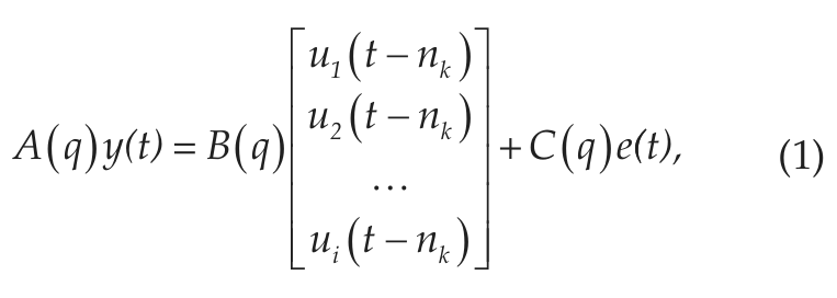
A (q) y (t) = B (q) [\begin{matrix} u_{1} (t - n_{k}) \\ u_{2} (t - n_{k}) \\ \dots \\ u_{i} (t - n_{k}) \end{matrix}] + C (q) e (t),

(1)

where u(t-n_k) are the delayed inputs, y(t) is the output, e(t) is the noise model, and A,B,C are the model coefficients. The term n_k corresponds to the delay, and q is the backward shift operator. The variable e(t) is a white-noise disturbance generated by the algorithm. It is uncorrelated with the input signals, is uncorrelated with itself, and has a constant variance over time. The model identifies long-term trends in the input signals (exogenous inputs), which are combined linearly to produce the desired output. The current output depends on previous inputs and delayed inputs, dictated by the model parameters n_b and n_k, respectively. As in AR models, past output values also influence the current output, with a delay n_a specified also by the model configuration. This implicit recursion takes into account the past context beyond the actual order of the model. Incorporating the MA portion, the model also includes a noise disturbance value, or stochastic white process, of order n_c. All these parameters determine the value of the model coefficients A,B,C (equations 2 -4):

A (q) = 1 + a_{1} q^{- 1} + a_{2} q^{- 2} + \dots + a_{n_{a}} q^{- n_{a}},

(2)

B (q) = [\begin{matrix} b_{11} + b_{12} q^{- 1} + \dots + b_{1 n_{b}} q^{- n_{b} + 1} \\ b_{21} + b_{22} q^{- 1} + \dots + b_{2 n_{b}} q^{- n_{b} + 1} \\ \dots \\ b_{i 1} + b_{i 2} q^{- 1} + \dots + b_{i n_{b}} q^{- n_{b} + 1} \end{matrix}],

(3)

C (q) = 1 + c_{1} q^{- 1} + c_{2} q^{- 2} + \dots + c_{n_{c}} q^{- n_{c}},

(4)

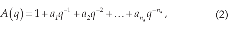
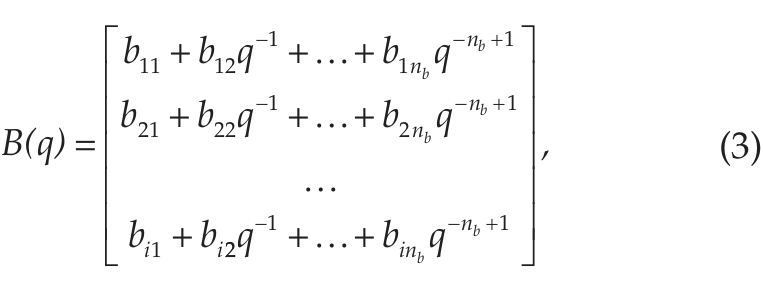
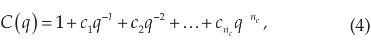
which are linearly combined to produce the output y(t). The values of the a,b,c weights were determined using an adaptive Gauss-Newton method (Wills and Ninness, 2008). The term B(q) can be considered a matrix of coefficients b, with the number of columns determined by the n_b parameter and the number of rows determined by the number of input signals. As mentioned previously, the output of the model is influenced not only by the input and delayed input but also by a delayed output. This relation can be illustrated in the flowchart depicted in Figure 1.

Figure 1.

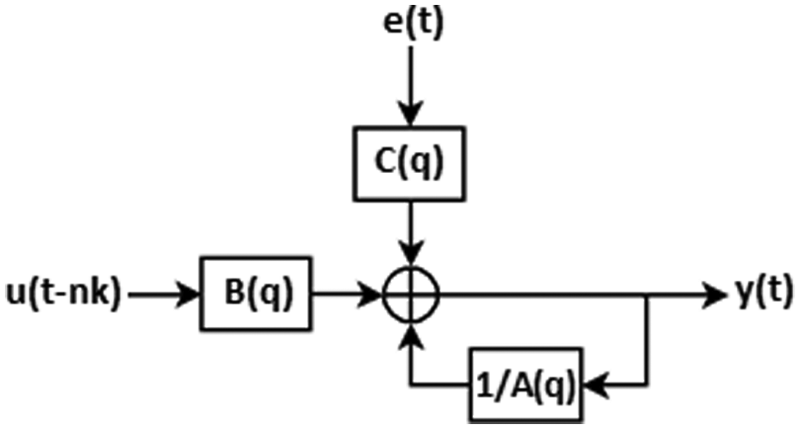
Flowchart of the ARMAX model.

Model Parameters and Testing

In statistical machine learning, the goal is to construct a system that is able to learn to solve a problem given a set of example data containing inputs as well as their expected outputs. The example dataset can be used to select an appropriate model and to evaluate the performance that is expected from the model. The model selection can be done by training and validating the model using 1 of 2 methods. Given a large enough dataset, the data can be divided into a training set and a validation set. The model can then be trained using the training dataset and then applied to the unseen data from the validation set. If the dataset is not large enough to create 2 datasets, the cross-validation technique can be used. A common form of this technique is the leave-one-out cross-validation (LOOCV) (Stone, 1974). In this method, the model is trained using all but 1 sample, and then the validation is carried out using that left-out sample. This is then repeated by leaving out a different sample and training on the rest until all samples have been used for the validation. To carry out both the model selection and evaluation of the model performance, these methods need to be combined. One option is to have 3 datasets in which the first one is used for training, the second for validation, and the third for performance evaluation. A second option is to do a double cross-validation, which is essentially a cross-validation in which the data are divided into 3 subsets. The last possibility is using a combination of the 2 aforementioned techniques. The model selection can be carried out using the cross-validation technique applied on the training set, and a second independent dataset is used for the performance evaluation. The model selection and performance evaluation in this study were carried out using this last method.

Prior to training the ARMAX model, the input signals were preprocessed and scaled. The activity and light data were sampled at 1 sample per minute. The RR intervals extracted from the ECG signal (256 Hz) were naturally nonuniformly sampled; therefore, the signal was resampled to match the sampling frequency of the other signals. A median filter, with a window size of 15 minutes, was applied to smooth the signals and remove noise. Twenty-four-hour segments of each signal were extracted, aligned, and standardized. Standardization was done using equation 5:

x_{s t a n d} = (x - x_{m e a n}) / x_{s d} .

(5)

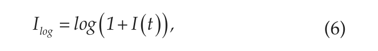
Various processing schemes of the light trace were applied. First of all, clipping of the light intensity values at 1000 lx was compared to no clipping. Furthermore, the light trace was processed using 3 different techniques, and the performance in the model of each was compared, namely the light intensity as measured by the Actiwatch Spectrum in lux, using a logarithmic compression (equation 6) (Dumont and Beaulieu, 2007b) or using a power compression (equation 7) (Kronauer et al., 1999; St. Hilaire et al., 2007). These 3 light traces were individually used in the training of the models, and the performance of each was compared:

I_{l o g} = l o g (1 + I (t)),

(6)

I_{p o w} = I {(t)}^{0.5} .

(7)

The reference output signal was a 24-hour cosine with an amplitude of 1, period of 24 hours, and phase equal to the DLMO. When using a time series model such as the ARMAX, it is necessary that the input and output vectors are of the same length. Given that the input vector is a 24-hour segment, the output vector must also comprise 24 hours of data. Since the parameter of interest was phase, the simplest way to express phase as a circadian signal is with a cosine having this particular phase shift. Using higher harmonics to compose a melatonin profile would require a priori knowledge of representative frequencies as well as amplitudes. This DLMO-coded cosine (equation 8) was used as the output signal in which the maximum of the cosine corresponds to the DLMO of the participant:

y (t) = \cos (2 π f t - φ_{D L M O}) .

(8)

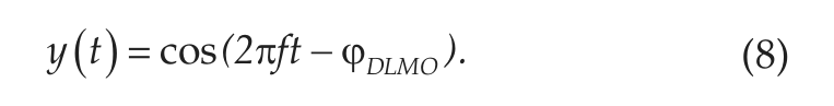
The output of the ARMAX model was then fitted using a cosinor analysis, from which the maximum was obtained. This maximum was used as the DLMO prediction (DLMO_pred), which was compared to the DLMO calculated from the melatonin profile. Figure 2 provides a flowchart of the model.

Figure 2.

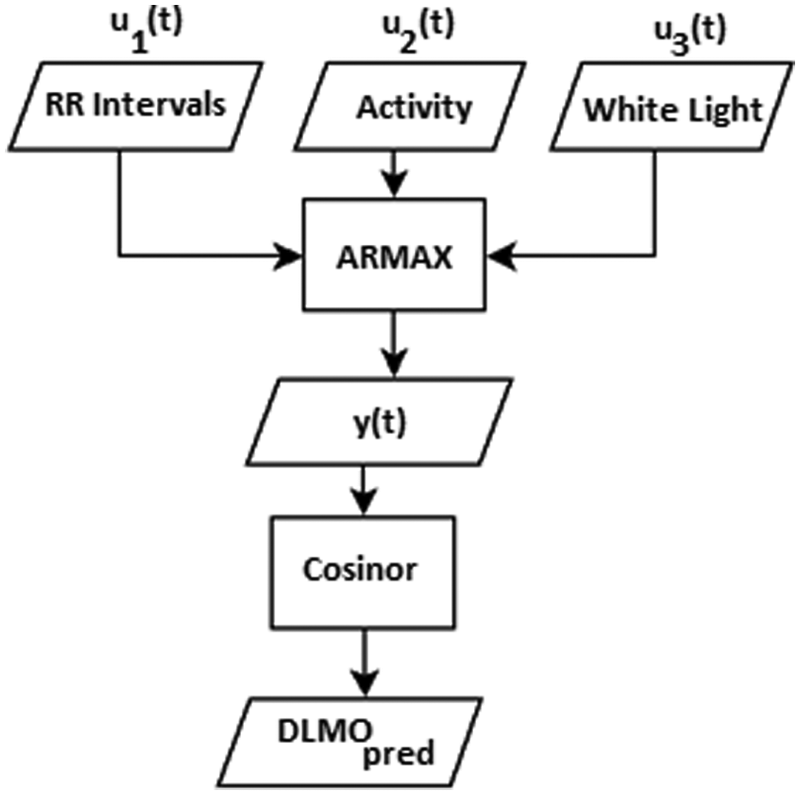
Flowchart of the DLMO prediction model.

The ARMAX model was trained with dataset A and evaluated using dataset B. The best set of coefficients and delays was determined using LOOCV by training on 10 participants and evaluating the results on 1. Having determined the best model parameters based on the Akaike information criterion (AIC) and SD of the error, the model performance was evaluated using dataset B. Using these criteria, the best model in the training data was the one using RR intervals and light with an order configuration of n_a = 3, n_b = (3,3), n_c = 1, and n_k = (3,3). Building upon the description of the ARMAX model, this model configuration can be interpreted as a third-order model, which looks at 3 points in each of the input signals (n_b) and 3 points in the output itself (n_a). The model includes a delay (dead time) of 3 points for the input data (n_k). There are 2 values for n_b each with a value of 3, indicating that the same number of points is taken into account from both input signal streams, each with the same dead time n_k. The models were not retrained or modified in any way; the signals from dataset B were simply processed in the same manner as those from dataset A. This was done using all possible input combinations of RR intervals, activity, each of the 3 processed light signals with and without clipping, and the previously described DLMO-coded cosine output signal, resulting in 27 ARMAX models of a third order. All processing, modeling, and analysis were done using Matlab version R2010b.

A sample of each of the input signals and the DLMO-coded cosine signal together with the model output can be found in Figure 3. The signals have been preprocessed as outlined before and standardized, and the light signal was compressed using the power law equation (7) with no clipping.

Figure 3.

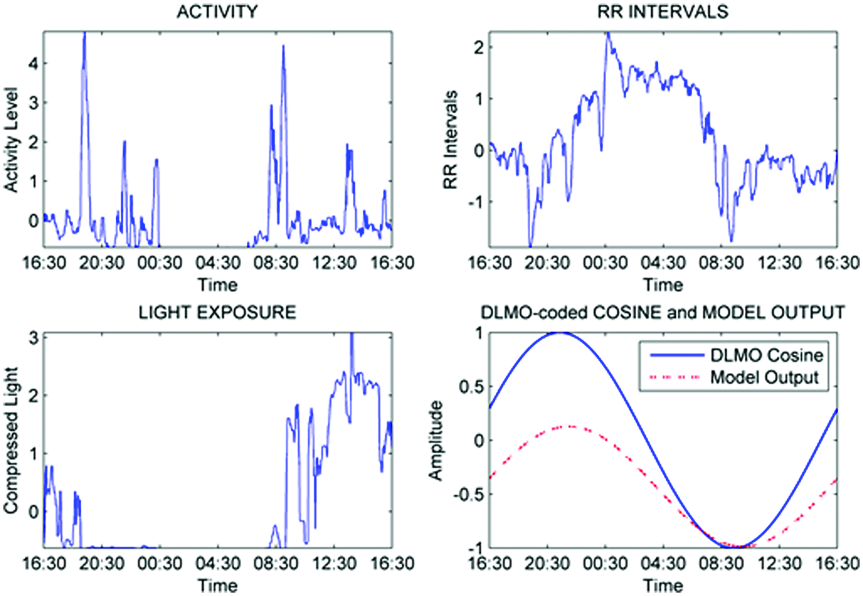
Sample input and output signals.

Results

In dataset A, the heart rate measurement of 3 participants was excluded due to technical problems with the heart monitor. Of the 48 recordings of dataset B, 6 were excluded due to technical problems with the ECG monitors, 2 participants failed to comply with the saliva sampling protocol, and 4 melatonin curves were excluded due to melatonin measurement errors.

There was no significant difference (p = 0.72) between the mean DLMO values for dataset A and B: 2148 ± 0106 h and 2150 ± 0048 h, respectively. However, in line with the inclusion criteria, there was a significant difference (p < 0.01) in the hMS times. Participants in dataset A and dataset B had a mean midsleep time of 0506 ± 0047 h and 0349 ± 0045 h, respectively. Hence, the angle of entrainment was longer on average by about 1 hour for the subjects of dataset A than for those in dataset B. In addition, there was a significant difference (p = 0.01) between the mean age of both datasets (23.7 ± 1.8 years and 26.7 ± 4.0 years, respectively), but no significant difference (p = 0.98) was found between the mean BMI: 21.7 ± 2.5 and 21.8 ± 2.6, respectively.

Dataset B included 2 RR interval samples over 24 hours from each participant. Both instances were recorded in the same manner, and there was no explicit element of intervention in the protocol that would lead to a difference in the DLMO values. However, during this 1-week period in between ECG recordings, lighting conditions, sleep schedules, and essentially any other factors relevant to circadian timing could be different. Therefore, to eliminate the effects that these differences could have had on the comparison of phase estimations, the 2 sessions were randomized. This means that the 2 sessions were assigned to 2 groups randomly while ensuring that each participant was present in each group only once. The 2 sessions were analyzed separately, and the average of the 2 is presented here. The estimate errors were not significantly different (p < 0.05), and therefore, they could be combined into 1 average error and 1 average SD. The different scaling and light processing schemes were tested individually; however, only the results of the best performing scaling and light traces are shown. To give a comparison on the performance of the models, the 2 sessions for the validation dataset were reduced to include only the common participants, resulting in a total of 16 participants, as opposed to 17 and 19 for the 2 sessions, respectively. Nevertheless, the evaluation was also run using all participants, and the results were not significantly different for any of the models (0.54 ≤ p ≤ 1.0)

From the 27 models, only 7 models are presented since only the best performing scaling and light processing schemes are shown. The best performing models were selected based on the AIC, resulting in models with varying levels of complexity. Scatterplots of the expected DLMO and the predicted DLMO for the 7 different models are shown in Figure 4. The third-order ARMAX models yielded a compact representation of signal processes, ranging from 7 to 15 coefficients depending on the number of signals used.

Figure 4.

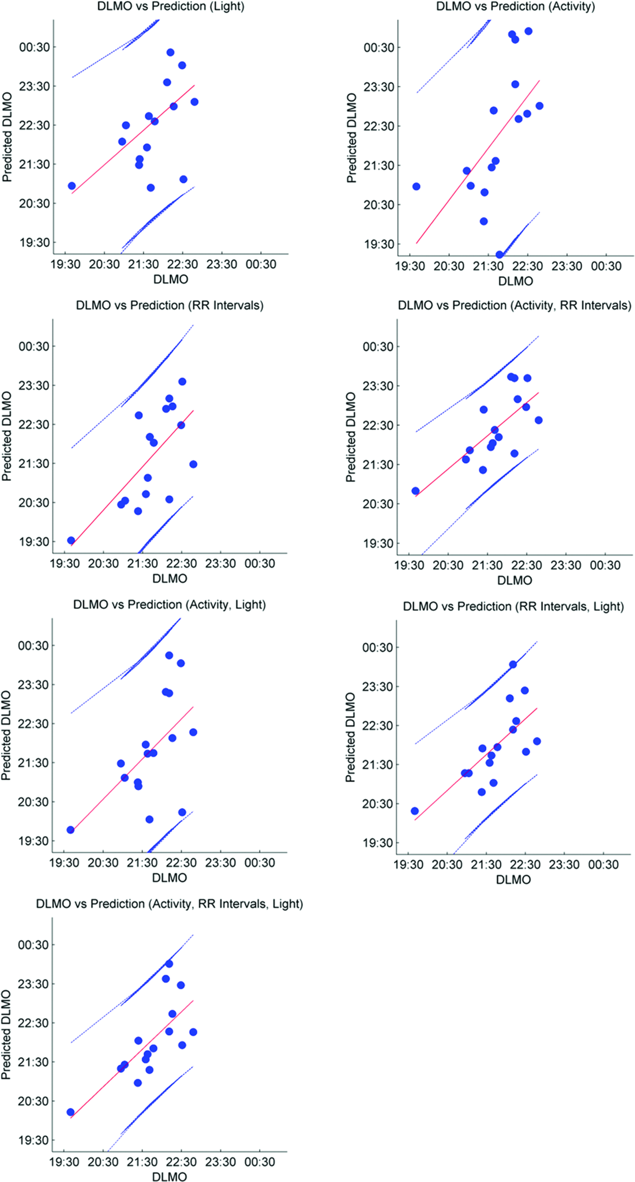
Measured DLMO versus predicted DLMO for each subject using the 7 ARMAX models presented in Table 1. Only 1 of the 2 sessions is shown. The plot shows the linear fit (center line) and the ±95% confidence interval.

Table 1.

Average error (bias) defined as the difference between the expected DLMO and the predicted DLMO and SD of the error for the ARMAX models using activity, RR intervals, and light.

Signals Used in Model	Error, Mean ± SD, min	Pearson R	p Value
Light_pow	−37 ± 56	0.548	0.03
Activity	−8 ± 81	0.307	0.47
RR intervals	23 ± 56	0.650	<0.01
Activity, RR intervals	−27 ± 40	0.654	0.01
Activity, light_log	6 ± 57	0.606	0.01
RR intervals, light_pow	2 ± 39	0.712	<0.01
Activity, RR intervals, light_pow	−5 ± 39	0.722	<0.01

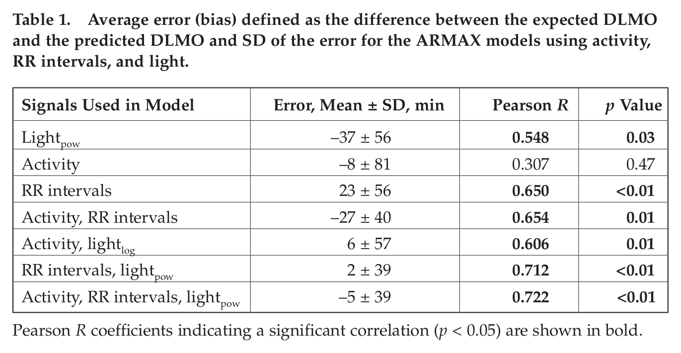
Pearson R coefficients indicating a significant correlation (p < 0.05) are shown in bold.

The average error can be thought of as a bias or a calibration factor that can be applied uniformly to the outputs. On the other hand, the SD of the error represents the error that can be expected among participants. Therefore, the SD of the error provides a more representative evaluation of the performance of the model, as it shows the range of errors that can be expected.

The best performing model was determined to be the RR interval and light model based on the SD of the error and the Pearson correlation. Figure 5 shows the Bland-Altman plots (Altman and Bland, 1983; Bland and Altman, 1986, 1999) for this model applied to the 2 sessions. Bland-Altman plots are a standard method of comparing 2 measurements and determining the agreement between the 2. In this case, the plots compare the output of the model to the reference values of DLMO. The systematic bias is displayed as a solid line, which in this case corresponds to 4 minutes for session 1 and 0 minutes for session 2 (an average bias of 2 minutes). The SDs of the error are also shown with dashed lines at 36 and 42 minutes for sessions 1 and 2, respectively (39 minutes on average). In addition, the 95% limits of agreement showing the magnitude of the error that can be expected for 95% of the population are shown with dash-dotted lines. This allows for easily assessing the presence of outliers.

Figure 5.

Bland-Altman plots of the model with the lowest error and SD of the error. The solid line labeled “Mean Diff” shows the mean difference between the predicted DLMO and the measured DLMO (bias), the dashed lines labeled “Mean Diff ± SD” show the mean ± 1 SD, and the dashed lines labeled “Mean Diff ± 1.96*SD” show the 95% limits of agreement defined as the mean difference ± 1.96*SD. (A) The results of the model for session 1 with an error of 4 ± 36 minutes. (B) The results of the model for session 2 with an error of 0 ± 42 minutes.

Discussion

Phase estimation of the human circadian pacemaker is possible through the use of various physiological signals, which rely strongly on the master circadian clock. However, to arrive at an accurate estimate without using DLMO, prolonged data collections are necessary. We presented a method that is able to predict human circadian phase based on only 24 hours of data recorded in ambulatory conditions. Models using combinations of activity, light, and RR intervals were presented, and it was found that the inclusion of RR intervals yielded the best performing models.

The RR intervals, or more broadly speaking HRV, are dependent on the autonomic nervous system, which follows a circadian cycle. This circadian output signal is highly prone to masking effects, making it difficult to assess the pure circadian component of the SCN that is driving it. The ARMAX model structure presented here was able to extract circadian information from the different signals, particularly the RR interval signal, with only 24 hours of data. The masking effects from daily ambulatory activity did not degrade the result, given the model’s MA smoothing coupled with its AR behavior. Through statistical machine learning, the ARMAX model determined the weight of each signal as well as the magnitude of the coefficients. In all models combining 2 or 3 signals, the RR interval signal was given the largest weight.

The gold standard of assessing circadian phase is DLMO due to its close dependence on the circadian pacemaker and its robustness (Lewy and Sack, 1989). In the evaluation part of this study, 2 melatonin measurements were taken 1 week apart. One cannot assume that given the ambulatory conditions and the lack of behavioral constraints, DLMO would remain constant during this time. Nevertheless, as a test of the prediction power of using one DLMO to estimate a second DLMO, the first session was compared to the second session. It was found that this estimation yielded an error of −12 ± 28 minutes (R = 0.841, p < 0.01). If the 2 DLMO values were assessed in successive days, one could assume that the correlation would probably be higher. However, using one DLMO value to estimate a second DLMO, without considering the data between the 2 sessions, is not ideal, given the nature of ambulatory conditions and the lack of behavioral restrictions that could lead to shifts that cannot be easily assessed.

Systematically evaluating the results obtained from the different models, it can be seen that the models using individual signals yielded large SD of the error values, with the RR intervals producing the lowest at 56 minutes (R = 0.650, p < 0.01). Combining signals resulted in an improvement of the results, as would be expected from the inclusion of more information. However, the largest improvement was achieved from the combination of RR intervals and light. Light alone yielded a prediction error of 37 ± 56 minutes (R = 0.548, p = 0.03), and RR intervals alone yielded a prediction error of −23 ± 56 minutes (R = 0.650, p < 0.01). When combining the 2 signals, the prediction error dropped to 2 ± 39 minutes (R = 0.712, p < 0.01). The combination of all 3 signals resulted in prediction errors very similar to those of the RR intervals and light model, with an error of −5 ± 39 minutes (R = 0.722, p < 0.01). Therefore, the inclusion of activity did not provide the model with new information that could improve the estimates of circadian phase. To determine which of the signals provided redundant information, the covariance between signals was calculated. The covariance between the activity and light traces was 0.11, while the covariance between the activity and RR intervals was −0.68. This suggests that the information found in the activity signal was already well represented by the RR interval signal. Depending on the randomization of the 2 recording sessions, different SDs of the error were obtained. The average error was always constant. The randomization was iterated 400 times, and the average SD of the error along with the 95% confidence intervals of the SD of the error was calculated. For the selected model, the 95% confidence interval was ±3 minutes, resulting in a range of SDs of the error of 36 to 42 minutes. Given the progression of the improvement, it seems that the RR intervals alone provided the bulk of the information for the phase estimation. Once the other signals were included, the estimates were shifted in time, yielding lower bias values and an improvement in the SD of the errors. As previously mentioned, the RR intervals were given the largest weighting by the statistical model training. The other signals provided a way of fine-tuning the phase estimates given their lower weightings.

The results showed that the model with RR intervals and light yielded the best estimates of circadian phase. The circadian dynamics of HRV have been assessed in various studies such as those by Scheer et al. (1999), van Eekelen et al. (2004), Vandewalle et al. (2007), and recently Boudreau et al. (2012). However, its relevance to phase estimation has been underestimated. The results presented here show that meaningful circadian information can be extracted from a 24-hour segment of RR intervals and that this information can be used to estimate circadian phase, given the appropriate type of model is used. In addition, incorporating light into the model resulted in improvements of the phase estimates. However, using these signals alone did not reveal reliable phase estimations, despite the light’s position as the primary zeitgeber. This is expected as the light trace alone contains no information regarding the intrinsic period of the person or the dynamics of the response to light. As a common characteristic in previously mentioned circadian phase estimation models, it seems that it is rather the combined use of endogenous circadian signals such as HRV, and an environmental entrainment signal such as light, that is able to yield reliable estimates of the state of the circadian clock.

Conclusion

The current model, which uses RR intervals and light to estimate circadian phase, has been tested in normal ambulatory conditions. Given the interaction of the signals, it would be interesting to test the effects of light therapy and whether this can be accurately modeled using an AR model as presented here. In addition, other subject populations such as shift workers or pathological patients can be addressed to test the limits of the model and determine the model’s applicability to other conditions of interest.

Heart rate variability is a very rich signal that is often studied both in the time and the frequency domain. This study has focused only on the temporal sequence of RR intervals. Therefore, further work can be carried out, taking into account the spectral information, which is more common practice, especially in the cardiology domain. Although the current models showed the importance of the RR intervals as a possible predictor of circadian phase, the magnitude of the circadian component in this signal is still not clear. Therefore, a more in-depth analysis of HRV from a chronobiological point of view could shed light into the mechanism by which the circadian pacemaker influences HRV.

In addition to the signals tested here, other signals that can be collected noninvasively can be evaluated in future models. Skin temperature has been shown to possess a circadian rhythm (Krauchi and Wirz-Justice, 1994; Krauchi et al., 2000) and has also been used in a linear regression model (Kolodyazhniy et al., 2011) and a nonlinear neural network model (Kolodyazhniy et al., 2012) to estimate circadian phase. Nevertheless, when considering other signals, emphasis must be given to the use of signals collected noninvasively, in ambulatory conditions, and for periods of time in the order of 24 hours. This is a need that is still present, and it remains an ongoing challenge to provide accurate circadian phase estimations readily and reliably, with as little patient burden as possible. Providing practical methods that are less time consuming and less expensive, while still delivering accurate results like the one we presented here, can help advance chronotherapeutic and chronomedical applications.

Footnotes

Acknowledgements

This work was supported by the EU Marie Curie Network iCareNet under grant number 264738. The authors thank Marijke Gordijn and Moniek Geerdink of the University of Groningen for the collection of dataset A and the analysis of the melatonin samples.

Conflict of Interest Statement

The author(s) have no potential conflicts of interest with respect to the research, authorship, and/or publication of this article.

References

Altman

Bland

(1983) Measurement in medicine: the analysis of method comparison studies. Statistician 32(3):307-317.

Anders

Vollenweider

Cann

Hofstetter

Flammer

Orgül

Kräuchi

(2010) Heart-rate variability in women during 40-hour prolonged wakefulness. Chronobiol Int 27(8):1609-1628.

Aoyagi

Ohashi

Yamamoto

(2003) Frequency characteristics of long-term heart rate variability during constant-routine protocol. Am J Physiol Regul Integr Comp Physiol 285(1):171-176.

Beck

Steer

Ball

Ranieri

(1996) Comparison of Beck Depression Inventories-IA and -II in psychiatric outpatients. J Pers Assess 67(3):588-597.

Bilan

Witczak

Palusiński

Myśliński

Hanzlik

(2005) Circadian rhythm of spectral indices of heart rate variability in healthy subjects. J Electrocardiol 38(3):239-243.

Bland

Altman

(1999) Measuring agreement in method comparison studies. Stat Methods Med Res 8(2):135-160.

Bland

Altman

(1986) Statistical methods for assessing agreement between two methods of clinical measurement. Lancet 327(8476):307-310.

Boudreau

Yeh

Dumont

Boivin

(2012) A circadian rhythm in heart rate variability contributes to the increased cardiac sympathovagal response to awakening in the morning. Chronobiol Int 29(6):757-768.

Box

GEP

Jenkins

Reinsel

(2008) Time Series Analysis: Forecasting and Control. 4th ed. Hoboken, NJ: Wiley.

10.

Brown

Choe

Luithardt

Czeisler

(2000) A statistical model of the human core-temperature circadian rhythm. Am J Physiol Endocrinol Metab 279(3):E669-E683.

11.

Buijs Ruud

la Fleur

Wortel

Van Heyningen

Zuiddam

Mettenleiter

Kalsbeek

Nagai

Niijima

(2003) The suprachiasmatic nucleus balances sympathetic and parasympathetic output to peripheral organs through separate preautonomic neurons. J Comp Neurol 464(1):36-48.

12.

Czeisler

Kronauer

Allan

Duffy

Jewett

Brown

Ronda

(1989) Bright light induction of strong (type 0) resetting of the human circadian pacemaker. Science 244(4910):1328-1333.

13.

Dumont

Beaulieu

(2007) Light exposure in the natural environment: relevance to mood and sleep disorders. Sleep Med 8(6):557-565.

14.

Freitas

Lago

Puig

Carvalho

Costa

de Freitas

(1997) Circadian heart rate variability rhythm in shift workers. J Electrocardiol 30(1):39-44.

15.

Ganesh

Krishna

Hariprasad

Rau

(2011) Review on models for generalized predictive controller. First International Conference on Computer Science, Engineering and Applications. Chennai, India, July 15-17. pp 418-424.

16.

Geerdink

Beersma

DGM

Hommes

Gordijn

MCM

(2011) Phase advancing the human circadian system with short pulses (30 min) of blue light exposure. Abstracts of the XII Congress of the European Biological Rhythms Society. Abstract 136. August 20-26, Oxford, UK.

17.

Gompper

Bromundt

Orgül

Flammer

Kräuchi

(2010) Phase relationship between skin temperature and sleep-wake rhythms in women with vascular dysregulation and controls under real-life conditions. Chronobiol Int 27(9-10):1778-1796.

18.

Hannan

(1976) The identification and parameterization of Armax and state space forms. Econometrica 44(4):713.

19.

Hayano

Sakakibara

Yamada

Kamiya

Fujinami

Yokoyama

Watanabe

Takata

(1990) Diurnal variations in vagal and sympathetic cardiac control. Am J Physiol 258(3 Pt 2):H642-H646.

20.

Hofstra

de Weerd

(2008) How to assess circadian rhythm in humans: a review of literature. Epilepsy Behav 13(3):438-444.

21.

Ivanov

Hilton

Chen

Ayers

Stanley

Shea

(2004) Endogenous circadian rhythm in an index of cardiac vulnerability independent of changes in behavior. PNAS 101(52):18223-18227.

22.

Jewett

Forger

Kronauer

(1999) Revised limit cycle oscillator model of human circadian pacemaker. J Biol Rhythms 14(6):493-499.

23.

Klerman

Gershengorn

Duffy

Kronauer

(2002) Comparisons of the variability of three markers of the human circadian pacemaker. J Biol Rhythms 17(2):181-193.

24.

Klerman

Rimmer

Dijk

Kronauer

Rizzo

Czeisler

(1998) Nonphotic entrainment of the human circadian pacemaker. Am J Physiol 274(4 Pt 2):R991-R996.

25.

Kolodyazhniy

Späti

Frey

Götz

Wirz-Justice

Krauchi

Cajochen

Wilhelm

(2011) Estimation of human circadian phase via a multichannel ambulatory monitoring system and a multiple regression model. J Biol Rhythms 26(1):55-67.

26.

Kolodyazhniy

Späti

Frey

Götz

Wirz-Justice

Krauchi

Cajochen

Wilhem

(2012) An improved method for estimating human circadian phase derived from multichannel ambulatory monitoring and artificial neural networks. Chronobiol Int 29(8):1078-1097.

27.

Krauchi

Cajochen

Werth

Wirz-Justice

(2000) Functional link between distal vasodilation and sleep-onset latency? Am J Physiol Regul Integr Comp Physiol 278:741-748.

28.

Krauchi

Wirz-Justice

(1994) Circadian rhythm of heat production, heart rate, and skin and core temperature under unmasking conditions in men. Am J Physiol Regul Integr Comp Physiol 267:819-829.

29.

Kronauer

Forger

Jewett

(1999) Quantifying human circadian pacemaker response to brief, extended, and repeated light stimuli over the photopic range. J Biol Rhythms 14(6):500-515.

30.

Kubota

Uchiyama

Suzuki

Shibui

Kim

Tan

Tagaya

Okawa

Inoue

(2002) Effects of nocturnal bright light on saliva melatonin, core body temperature and sleep propensity rhythms in human subjects. Neurosci Res 42(2):115-122.

31.

Lack

Bramwell

Wright

Kemp

(2007) Morning blue light can advance the melatonin rhythm in mild delayed sleep phase syndrome. Sleep Biol Rhythms 5(1):78-80.

32.

Levi

(2006) Chronotherapeutics: the relevance of timing in cancer therapy. Cancer Causes Control 17(4):611-621.

33.

Levi

(2008) The circadian timing system: a coordinator of life processes: chronobiological investigations. Implications for the rhythmic delivery of cancer therapeutics. IEEE Eng Med Biol Mag 27(1):17-19.

34.

Levi

Okyar

(2011) Circadian clocks and drug delivery systems: impact and opportunities in chronotherapeutics. Expert Opin Drug Deliv 8(12): 1535-1541.

35.

Lewy

Sack

(1989) The dim light melatonin onset as a marker for circadian phase position. Chronobiol Int 6(1):93-102.

36.

Mott

Dumont

Boivin

Mollicone

(2011) Model-based human circadian phase estimation using a particle filter. IEEE Trans Biomed Eng 58(5):1325-1336.

37.

Pandi-Perumal

Smits

Spence

Srinivasan

Cardinali

Lowe

Kayumov

(2007) Dim light melatonin onset (DLMO): a tool for the analysis of circadian phase in human sleep and chronobiological disorders. Prog Neuropsychopharmacol Biol Psychiatry 31(1):1-11.

38.

Perrott

Cohen

(1996) An efficient approach to ARMA modeling of biological systems with multiple inputs and delays. IEEE Trans Biomed Eng 43(1):1-14.

39.

Roenneberg

Wirz-Justice

Merrow

(2003) Life between clocks: daily temporal patterns of human chronotypes. J Biol Rhythms 18(1):80-90.

40.

Scheer

van Doornen

Buijs

(1999) Light and diurnal cycle affect human heart rate: possible role for the circadian pacemaker. J Biol Rhythms 14(3):202-212.

41.

Scheer

FAJL

Van Doornen

LJP

Buijs

(2004) Light and diurnal cycle affect autonomic cardiac balance in human: possible role for the biological clock. Auton Neurosci 110(1):44-48.

42.

Smith

Cullnan

Eastman

(2008) Shaping the light/dark pattern for circadian adaptation to night shift work. Physiol Behav 95(3):449-456.

43.

St. Hilaire

Gronfier

Zeitzer

Klerman

(2007a) A physiologically based mathematical model of melatonin including ocular light suppression and interactions with the circadian pacemaker. J Pineal Res 43(3):294-304.

44.

St. Hilaire

Klerman

Khalsa

SBS

Wright

Jr. Czeisler

Kronauer

(2007b) Addition of a non-photic component to a light-based mathematical model of the human circadian pacemaker. J Theor Biol 247(4):583-599.

45.

Stone

(1974) Cross-validatory choice and assessment of statistical predictions. J R Stat Soc Series B 36(2):111-147.

46.

Task Force of the European Society of Cardiology and the North American Society of Pacing and Electrophysiology (1996) Heart rate variability: standards of measurement, physiological interpretation and clinical use. Circulation 93(5):1043-1065.

47.

Tham

(1999) Dynamic Models for Controller Design. Newcastle upon Tyne, UK: University of Newcastle upon Tyne.

48.

van Eekelen

APJ

Houtveen

Kerkhof

(2004) Circadian variation in base rate measures of cardiac autonomic activity. Eur J Appl Physiol 93(1-2):39-46.

49.

Van Someren

EJW

Nagtegaal

(2007) Improving melatonin circadian phase estimates. Sleep Med 8(6):590-601.

50.

Vandewalle

Middleton

Rajaratnam

SMW

Stone

Thorleifsdottir

Arendt

Dijk

D-J

(2007) Robust circadian rhythm in heart rate and its variability: influence of exogenous melatonin and photoperiod. J Sleep Res 16(2):148-155.

51.

Weinert

(2010) Circadian temperature variation and ageing. Ageing Res Rev 9(1):51-60.

52.

Wills

Ninness

(2008) On gradient-based search for multivariable system estimates. IEEE Trans Autom Control 53(1):298-306.

53.

Wirz-Justice

(2007) How to measure circadian rhythms in humans. Medicographia 29(1):84-90.

Human Circadian Phase Estimation from Signals Collected in Ambulatory Conditions Using an Autoregressive Model

Abstract

Keywords

Materials and Methods

Subjects and Protocol

ARMAX Model

Model Parameters and Testing

Results

Discussion

Conclusion

Footnotes

Acknowledgements

Conflict of Interest Statement

References