Wavelet Meets Actogram

Abstract

A variety of methods to determine phase markers and period length from experimental data sets have traditionally assumed a rhythm of fixed period and amplitude. But most biological oscillations exhibit fluctuations in both period and amplitude, leading to the recent interest in the application of wavelet transforms that can measure how rhythms vary over time. Here we examine how wavelet-based methods can be extended to the analysis of conventional actograms, including the detection of onsets in circadian activity and temperature rhythms of rodents.

Determining free-running rhythm period length (τ) from experimental data sets is an essential task for almost everyone engaged in biological rhythm research. Traditionally, this has been done using methods that rely on sinusoidal waveforms of fixed frequencies and that assume rhythms of constant period and amplitude over time (e.g., the Fourier periodogram). Recently, wavelet transforms—a powerful type of time-frequency analysis that can measure how frequencies vary over time in a time series—have been used as effective tools for analyzing circadian rhythmicity, especially as applied to oscillating bioluminescent cells. Wavelet analyses have been valuable for studying variability in period and amplitude, characterizing rhythmicity at different time scales (Chan et al, 2000), and removing trend and noise (for review and references, including the underlying mathematics, see Leise and Harrington, 2011).

Here we show how we have used wavelets to measure the phase and period of behavioral rhythms. For more than 85 years (Johnson, 1926), such rhythms usually have been graphed and analyzed as actograms, in which activity (e.g., wheel running) over 24 or 48 h is plotted horizontally and succeeding days are stacked vertically. Historically, τ in behaving rodents typically has been determined on actograms by eye-fitting regression lines through successive daily activity onsets, because “the onset of activity . . . in the great majority of records is a more precise ‘marker’ of the rhythm than the end of activity” (Pittendrigh and Daan, 1976, p. 226); thus, a vast literature has accumulated on τ’s calculated using activity onset. To our knowledge, wavelet transforms have not yet been used to track circadian activity onsets, and here we describe how we have applied wavelets to objectively identify this phase marker.

Using Discrete Wavelet Transforms for Activity Rhythms

Given that activity onset on most actograms appears as a relatively sharp discontinuity, jumping from zero activity to a relatively high value, we used a maximal overlap discrete wavelet transform (DWT) with a Daubechies 4-tap orthogonal filter (shown in Suppl. Fig. S1), which identifies discontinuities in the first derivative of a signal (Percival and Walden, 2000). The DWT decomposes the original time series into components called details associated with different scales representing particular frequency bands (period ranges); see the supplementary online material or (Leise and Harrington, 2011). We can use the scale representing a circadian range of periods to identify circadian rhythm phase markers. With activity data binned at 15-min intervals, the circadian range [16-32 h] is represented by scale 6 (the period range associated with each wavelet scale depends on the binning interval).

We tried using this scale to determine both rhythm onset and peak; onset and peak phases determined in this way are plotted as green dots on the wheel-running actograms of a hamster (Fig. 1A) and a mouse (Fig. 1D) in constant darkness (DD). Scale 6–determined onset is obviously off; it is advanced by several hours from actual onset. Notably, unlike the true activity onset, the scale 6–determined onset phase moves in perfect lock-step with the scale 6–determined peak phase. The 2 green dots move in parallel as their phase is influenced by the nighttime activity waveform; they advance or delay when activity bout duration shortens or lengthens, respectively. This scale is better suited for identifying peak activity rather than onset of activity. So we need a more localized scale to mark activity onset.

Figure 1.

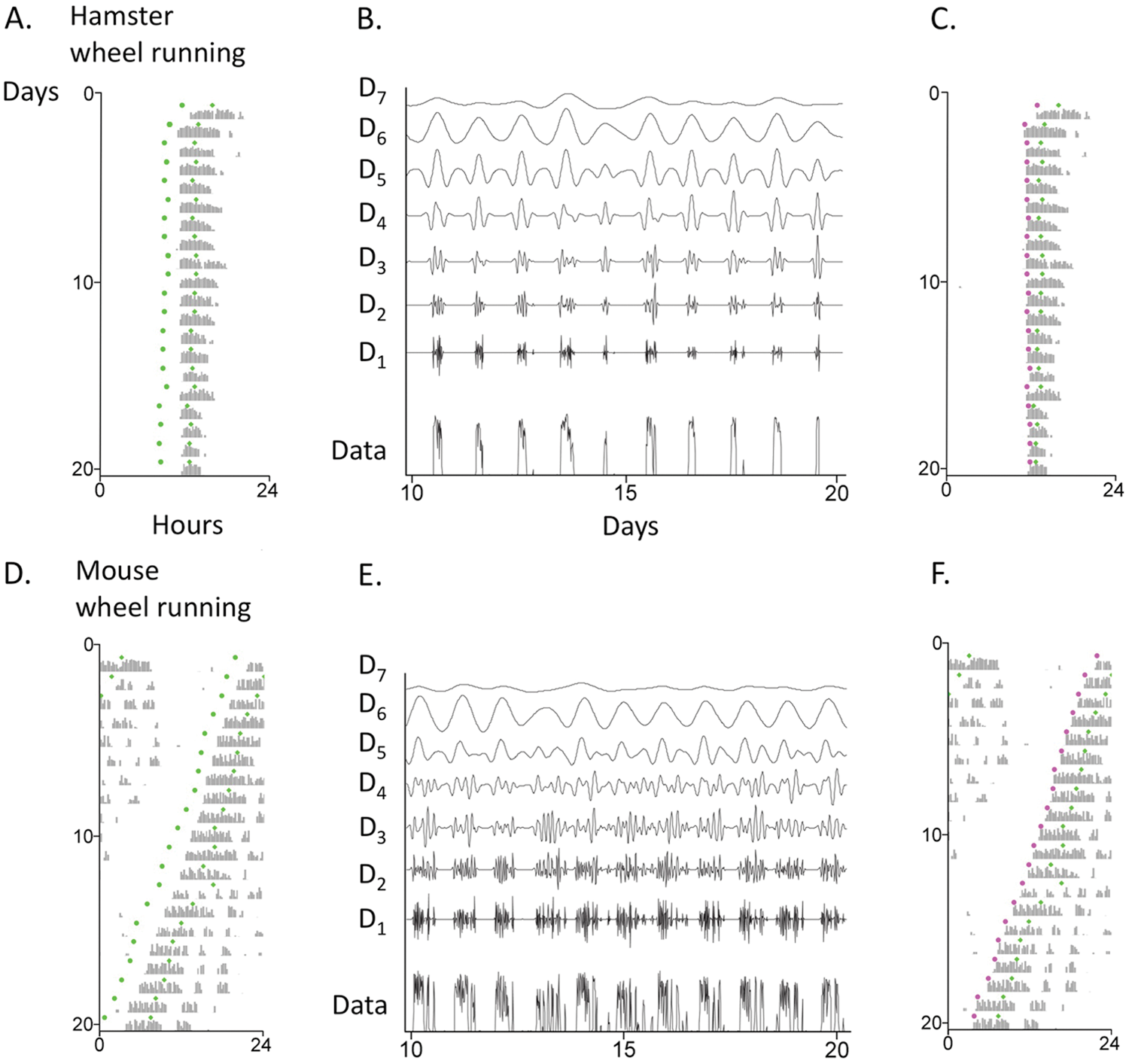
Examples of wheel-running actograms and DWT multiresolution analyses (MRA) displaying wavelet details (B, E) for a hamster (top) and mouse (bottom) in DD. That is, the DWT decomposed the activity into components associated with different period ranges. Within each MRA, each detail has mean zero and is plotted with the same axis scaling, so magnitudes can be directly compared. D₆-determined onset phases and peak phases are shown as green dots (A, D); D₃-determined onset phases and D₆-determined peak phases are shown as magenta and green dots, respectively (C, F).

Figures 1B and 1E show the hamster and mouse activity data from Figures 1A and 1D decomposed into DWT scales. Each successive scale doubles the associated periods and reveals different features of the activity rhythm. Here, for example, D₁ represents 0.5 to 1.0 h; D₃, 2 to 4 h; D₅, 8 to 16 h; D₆, 16 to 32 h. To choose which of these scales would be the most accurate for identifying activity onset, we constructed simulated data sets and tested the effects of noise, variable onset times, and gradual onsets. By using simulations for which we knew the actual onset times, we could calculate the error for each scale under each condition (data not shown). We concluded that D₃ seems a good choice, as long as activity onset is reasonably sharp rather than gradual in character; the prediction of activity onset with this method is little affected by white noise. Figures 1C and 1F show the revised phases of activity onsets (D₃; magenta) along with the phases of circadian peaks (D₆; green, as in Figs. 1A and 1D) on the hamster and mouse actograms.

Fig. 2 shows the course of D₃-determined onset phases and D₆-determined peak phases of another hamster’s wheel-running activity in DD, as well as the circadian amplitude measured by the D₆ peak. Note how the phase of the D₆-determined peak, but not that of the D₃-determined onset, is affected by the waveform of nighttime activity. Over the 80-day record, τ’s determined by D₃ onset (which we will call τ _o ) or by D₆ peak (which we will call τ _p ) are equivalent (23.94 or 23.93 h, respectively), but cycle-to-cycle variability is 3-fold greater for τ _p (S.D., 0.16 h for τ _o and 0.51 h for τ _p ), because the phase of the peak is influenced by the distribution and duration of wheel-running activity. The nonequivalence of τ _o and τ _p becomes manifest with shorter duration activity records. For the hamster in Fig. 2, the greatest difference in these 2 τs for any 10-day interval is 0.15 h; only after 60 days do they stabilize at their 80-day values.

Figure 2.

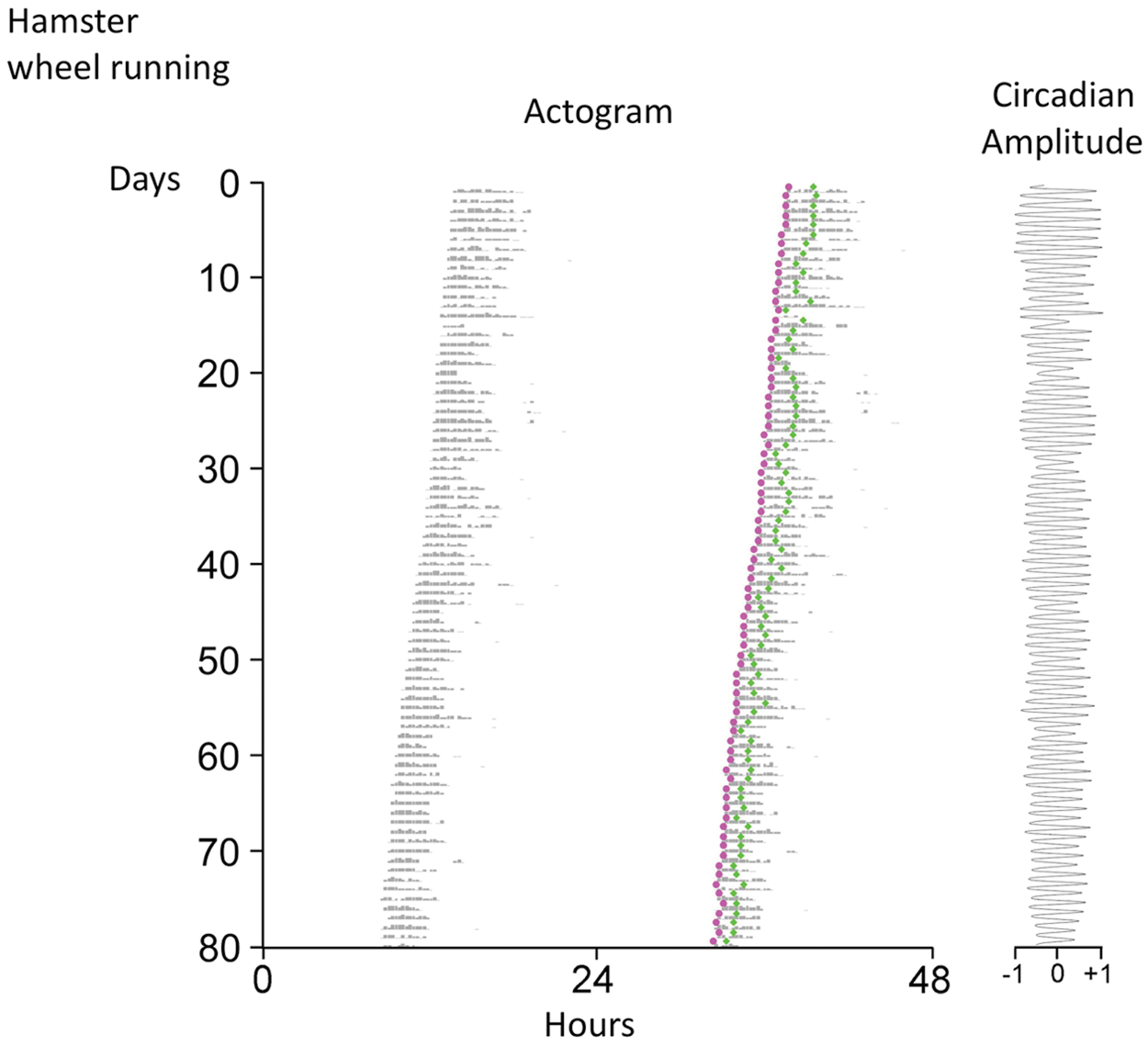
Example of a wheel-running actogram of a hamster in DD, with D₃-determined onset phases and D₆-determined peak phases shown as magenta and green dots, respectively; circadian amplitude, in normalized units, is measured by the D₆ peak.

Importantly, D₃-determined activity onsets appear to closely track dynamic changes in actual activity onsets, for example, if the wheel-running rhythm is shifted by a phase advance of the light–dark (LD) cycle (Fig. 3A) or when a “scalloped” pattern of activity onsets occurs with female estrous cycles (Morin et al., 1977) (Fig. 3B). In the latter case, D₃ correctly identifies the advanced phase of activity onset on the days preceding day 1 of the estrous cycle (day of vaginal discharge) (Fig. 3C) as well as the 4-day period of the cycle (Fig. 3D).

Figure 3.

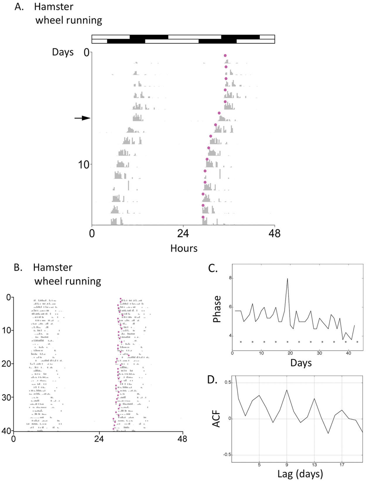
Examples of D₃-determined activity onsets for (A) a hamster subjected to a 6-h phase advance of a 14 h:10 h LD cycle on the day marked by the arrow, and (B) a female hamster in DD. For the latter, in C, activity onset (advances are down, delays are up) is plotted in relation to day 1 of the estrous cycle (day of vaginal discharge) (*), and in D, the autocorrelation function (ACF) indicates peaks at lags of 4 days, indicating a 4-day periodicity; for a time series with duration of length N, the autocorrelation measure is valid for lags up to N/2.

Last, we challenged our method to mark activity onsets of an activity rhythm that is less distinct than the wheel-running rhythm, specifically, the general locomotor activity rhythm as measured by a passive infrared detector. Here we found the limits of onset detection using the D₃ scale (Suppl. Fig. S2). If the sensitivity of our procedure is set at a relatively low level (the same as that already used in Figs. 1, 2, and 3; for description of “sensitivity,” see the Methods section), activity onset determination seems reasonably good for the hamster (Suppl. Fig. S2A) but quite poor for the mouse, with some of the D₃ onset phases coming too late on days when activity begins as a short-duration and/or low-amplitude burst (Suppl. Fig. S2C). Adjusting the sensitivity to a relatively higher level (see the Methods section) yields remarkably good activity onsets for the mouse (Suppl. Fig. S2D) but now hamster onsets are off, with some of the D₃ onset phases coming too early on days when little bursts of activity precede the main bout (Suppl. Fig. S2B). Thus, as a practical matter, for some rhythms in individual animals and particular species, attending to the effects of sensitivity thresholds will be important for properly interpreting wavelet data sets.

Using Continuous Wavelet Transforms for Temperature Rhythms

In addition to behavioral activity rhythms, body temperature rhythms can be longitudinally recorded using miniature implantable sensors; unlike activity rhythms, however, temperature rhythms do not include intervals with absent (zero) values or sharp discontinuities at onsets. The more continuous nature of temperature rhythm data suggests the use of continuous wavelet transforms (CWTs), which convolve the time series with scaled and translated wavelet functions in order to measure period and amplitude varying over time (Torrance and Compo, 1998). To determine the circadian component of the signal, we used the complex-valued Morlet wavelet function, as used by others for rhythms of cellular bioluminescence (Price et al., 2008; Baggs et al., 2009; Etchegaray et al., 2010; Meeker et al., 2011). The Morlet wavelet transform, however, failed to track rhythm onset (in the same way that the DWT D₆ detail failed to track activity onset), so we applied the real-valued Ricker wavelet function (the normalized second derivative of the Gaussian function), also known as the Mexican Hat wavelet, which is narrower in time scale than the Morlet wavelet function and better at capturing finer structure in the time-scale representation (see Suppl. Fig. S3 for graphs of these wavelet functions). Figure 4A shows the circadian rhythm of body temperature of a hamster running in a wheel in DD (“data,” as recorded by an intraperitoneal ibutton [Dallas Semiconductor DS1922, Maxim Integrated Products, Inc., Sunnyvale, CA]), along with the Morlet and Mexican Hat transforms of the data. In Figure 4B, the temperature rhythm is plotted in actogram format with Mexican Hat–determined onset phases and Morlet-determined peak phases denoted as magenta and green dots, respectively. DWT did not consistently perform as well as the CWT on these temperature data; similar CWT results were obtained in ibutton-implanted mice (not shown).

Figure 4.

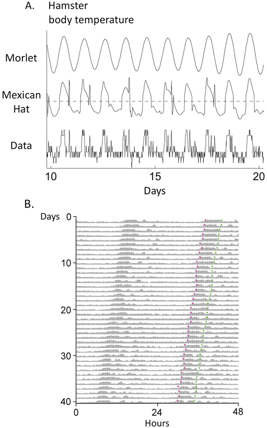
(A) Morlet and Mexican Hat wavelet transforms of the circadian body temperature rhythm (“data”) are shown for an exemplary hamster in DD; (B) data are plotted as an actogram, with Mexican Hat–determined onset phases and Morlet-determined peak phases shown as magenta and green dots, respectively.

We calculated the phase relationship between the onsets of rhythmic temperature (Mexican Hat) and wheel running (D₃) in a group of hamsters outfitted with ibuttons and running in wheels in DD. We found that the temperature rhythm phase leads the wheel-running rhythm by 94 ± 15 min (mean ± SD, n = 10 hamsters, average of 50 successive onsets per animal). DeCoursey et al. (1998) reported an average temperature phase lead of 59 min (with a range from 31 to 105 min) in hamsters in a 14 h:10 h LD cycle; these authors used the intersection of the daily temperature increase with the mean temperature level as the phase marker for onset on their raw temperature data (which we expect would occur later than the phase marker we use).

Discussion

As recognized previously, the application of wavelets to the analysis of circadian time series is a notable advance; wavelet transforms do not depend solely on underlying fixed sines and cosines, nor do they demand invariance of period and amplitude over time. The DWT can perform well at tasks like detecting abrupt changes and discarding noise and therefore offers great potential for analysis of activity data. The ability of a time-frequency analysis like the CWT to quantify cycle-to-cycle changes in the circadian amplitude of temperature rhythmicity is also an exciting prospect, given the emerging role of the temperature rhythm in coupling brain and body oscillators (Brown et al., 2002; Buhr et al., 2010). Here we present our application of discrete and continuous wavelet transforms for the analysis of conventional actograms, including the phase of activity onset, and we invite readers to consult the Methods section for instructions on how to use these procedures on their own data sets in their home laboratories.

A key point is that the free-running circadian period derived from the Daubechies filter or the Morlet function may not be equal to the traditional τ derived from a regression line along activity onsets. Of course, both are valid measures, but it is important to specify whether the period is τ _o (from the D₃ or Mexican Hat phase of rhythm onset) or τ _p (from the D₆ or Morlet phase of the circadian peak); the latter is influenced by the temporal architecture of the activity bout whereas the former is more localized in time. Although τ _o and τ _p provide similar values with extended data sets (e.g., 60 days), they differ when derived from shorter data sets typically used in circadian studies (e.g., 10 days). Hence the number of days being analyzed and the stability of the phase marker should be considered when applying these analyses, especially the cycle-to-cycle variability that characterizes τ _p .

An obvious and already known implication of our observations is that circadian activity rhythms include additional noncircadian time scales and that these scales (like the one underlying the abrupt timing of activity onset) likely reflect distinct neural substrates and mechanisms. Wavelet-based methods have great potential for providing tools to analyze patterns generated at these different scales. In general, biological rhythms, whether arising from activity, temperature, or other processes, can yield very rich data sets whose characteristics have not yet been fully plumbed, requiring new approaches to extract underlying patterns. This article provides a step toward expanding our toolbox of analysis methods for circadian data. We encourage further dialog and development of novel techniques, whether based on wavelets or on other mathematical and statistical methods, to continue expanding the field’s toolbox.

Methods

Computations

Numerical calculations were run on MATLAB 2012a (MathWorks, Natick, MA). Our customized MATLAB scripts are available at http://www.cs.amherst.edu/~tleise/CircadianWaveletAnalysis.html. We ask that readers please cite the present article when using these methods for their own work.

Discrete Wavelet Transform

For the DWT, our script calls on the WMTSA Wavelet Toolkit for MATLAB, developed by Charlie Cornish to accompany the book by Percival and Walden (2000). This package is freely available at http://www.atmos.washington.edu/~wmtsa/. The D₃ wavelet detail coefficients may have multiple peaks each day, marking onsets of different bouts of consolidated activity over the course of 24 h. Circadian rhythm activity onset should occur sometime between the middle of the circadian rest interval (nadir of the D₆ wavelet detail coefficients) and the peak of the circadian activity interval (peak of the D₆ detail coefficients), so we selected the D₃ peak that occurred between the D₆ nadir and peak. If more than one D₃ peak occurred in such an interval, we selected the largest peak unless an earlier peak reached an amplitude of at least a certain percentage of the largest peak. For the work reported here, we set this earlier peak percentage at either 60% (low sensitivity) or 37% (high sensitivity); that is, the higher sensitivity recognizes an earlier smaller D₃ peak as activity onset (note that commonly used methods also typically require adjustment of a parameter for optimal results). To account for the phase shift caused by the wavelet filter, 1.25 h was added to the phase of the D₃ peak to yield the phase of activity onset. This offset was determined through testing on both simulated and real activity data.

Continuous Wavelet Transform

For the CWT, our MATLAB script uses the wavelet software developed by Torrence and Compo (1998). This package is freely available at http://paos.colorado.edu/research/wavelets/software.html. For the Morlet-determined circadian peak phase, we ascertained the peak in the wavelet scalogram (which depicts the result of the CWT applied to the time series; the vertical axis represents frequency and the horizontal axis represents time; see Suppl. Fig. S4) for the period range 20 to 26 h, found the amplitude corresponding to the real part of the wavelet function, and obtained the phase at which the instantaneous amplitude of the oscillation reached maximum value. For the Mexican Hat–determined onset phase, we ascertained the peak in the wavelet scalogram for the entire period range at each instant of time and found the instantaneous predominant amplitude of the oscillation corresponding to this peak. Since Mexican Hat wavelet is a real-valued function that captures positive and negative portions of zero-centered oscillation as separate peaks, the phase at which the predominant component crossed zero was considered as rhythm onset.