
Abstract
Employing a cutting-edge quasi-experimental event study estimator from de Chaisemartin and D’Haultfœuille, the results of this paper indicate that light rail construction has a significant impact on reducing regional CO2 emissions per capita, and that these effects change dynamically for at least 20 years after construction. The paper categorizes these long-run effects into four phases of light rail operational effectiveness: an early “establishment” phase where observed effects on per capita emissions are relatively small, an “early growth” phase of increasing effectiveness, a “stagnation” phase where the benefits plateau, and a “maturity” phase of renewed effectiveness.
Introduction
In 2018, the Intergovernmental Panel on Climate Change (IPCC) concluded that global warming of 1.5°C—with serious attendant risks for a range of environmental and social systems—is likely to occur in the mid-twenty-first century if increases continue at the current pace. To forestall warming beyond 1.5°C, the IPCC estimates that global net CO2 emissions must decline by roughly 45 percent from 2010 levels by 2030 and reach net zero by 2050; to limit global warming to 2°C, CO2 emissions must decline by about 25 percent by 2030 and reach net zero around 2070 (2018). This of course implies that substantial reductions in CO2 must be achieved rapidly across many sectors of society.
Reductions in transportation-related emissions are particularly important, as nearly 12.9 billion metric tons of CO2 globally—some 37 percent of total CO2 emissions in 2018—were generated from petroleum use (S. C. Davis and Boundy 2020). In 2017, the U.S. transportation sector alone accounted for 1.8 billion metric tons of CO2 emissions (S. C. Davis and Boundy 2020). Of that, 84 percent of CO2 emissions (1.51 billion metric tons) come from passenger vehicles or heavy trucks, more than the entire emissions of the continents of Central & South America (1.24 billion metric tons) or Africa (1.37 billion metric tons) (S. C. Davis and Boundy 2020). Consequently, personal vehicle use is generally a primary component of the average U.S. resident’s carbon footprint (Greene and Plotkin 2011; Jones and Kammen 2013; The Nature Conservancy 2022).
Given these circumstances, a number of policy and planning interventions have been suggested to curb personal vehicle-related carbon emissions in the United States, including regional planning strategies to increase urban density and compactness (Deetjan et al. 2018; IPCC, 2018; Jones and Kammen 2013), increased electric vehicle adoption (Deetjan et al. 2018; Greene, Evans, and Hiestand 2013; IPCC 2018; Needell et al. 2016), pedestrian- and bicycle-oriented urban design (Deetjan et al. 2018), and investment in new public transit infrastructure and associated transit-oriented development (TOD) (Chatman et al. 2019; Deetjan et al. 2018; Ercan, Onat, and Tatari 2016; IPCC 2018; Kimball et al. 2013). Given the higher efficiency of transit vehicles and the subsequent land use impacts of TOD, transit systems have the potential to contribute to significant reductions in greenhouse gas (GHG) emissions (T. Davis and Hale 2007; McGraw et al. 2021; US EPA 2020). To that end, some twenty-five U.S. regions have engaged in new rail transit investment since 1980, seventeen of which were classified as light rail systems 1 (APTA 2019). While transit passenger miles have grown faster than highway vehicles miles since 1998, they have declined in recent years (e.g., a 2.5% drop between 2016-2017), as has the percentage of transit commuters, raising questions as to the long-term viability of the recently-built rail transit systems in reducing CO2 emissions (APTA 2019).
At the same time, much of the existing literature on the carbon-reduction potential of transportation and land use planning interventions involves modeling potential future behavior or calculating avoided emissions based on a set of existing assumptions (Ercan, Onat, and Tatari 2016; Hensher 2008; Kwan et al. 2017; Landis, Hsu, and Guerra 2019; McGraw et al. 2021; Mendoza, Buchert, and Lin 2019; Rojas-Rueda et al. 2012). Studies that empirically analyze the impact of these interventions generally focus on reductions to vehicle miles traveled (VMT) (Bailey, Mokhtarian, and Little 2008; Boarnet et al. 2020; Ewing and Hamidi 2014), or focus on the effect of population density or compact development on emissions (Gately, Hutyra, and Wing 2015; Glaeser and Kahn 2010; Gudipudi et al. 2016; Jones and Kammen 2013; Lee and Lee 2014; Mitchell et al. 2017). none directly assess the aggregate effects of the flurry of recent transit construction activity in the United States. Given the recently observed increase in on-road carbon emissions (Gately, Hutyra, and Wing 2019) despite increased transit investment, significant questions remain regarding the extent to which new transit systems reduce regional carbon emissions.
The purpose of this paper is to analyze the impact of thirteen light rail transit systems on regional on-road CO2 per capita (
The results show that construction of a light rail transit system fostered a significant reduction in regional on-road CO2 emissions per capita compared to the comparison group, and that these effects change dynamically for at least twenty years after construction. These effects can be roughly grouped into four phases or “eras” of light rail operations: an early “establishment” phase where observed effects on per capita emissions are relatively small, an “early growth” phase in which system operations and supporting investment and behavioral changes lead to increased effectiveness, a “stagnation” phase where the benefits plateau (likely due to the diminishing “novelty effect”) (Mohammad et al. 2013), and a “maturity” phase in which the magnitude of effects on emissions increase once again, perhaps due to long-run land use change, subsequent transit investment, and other structural regional adjustments.
While the choice of an appropriate comparison group for regions that built transit is difficult at this scale, the use of an event study approach in this context is novel, and the general pattern of results are robust across specifications. Thus, this paper provides a useful framework for future research on the causal effects of planning interventions and policies, building on a relatively small (but growing) body of existing quasi-experimental research in planning (Credit 2018; Ewing and Hamidi 2014; Park et al. 2020). And while further research—and/or additional data—is needed to further examine the role of specific transit system features on reducing regional emissions, as well as the role of supportive policies and behaviors at the regional scale, this paper provides important initial evidence for planners in favor of the idea that light rail transit systems have contributed to reductions in regional on-road CO2.
Literature Review
The existing literature dealing with the impact of transportation behavior on GHG emissions can be classified into four primary groups along three dimensions: general methods/approach (estimates of emissions savings vs. empirical data), the variable of interest (VMT vs. GHG emissions), and the object of analysis (transit systems or urban spatial structure more generally), as shown in the typology in Table 1. The first (1) group of prior work evaluates the observed role of transit on reducing vehicle miles traveled (VMT), from which impacts to GHG emissions can be inferred (Bailey, Mokhtarian, and Little 2008; Boarnet et al. 2020; Ewing and Hamidi 2014; Holtzclaw 2000; Newman and Kenworthy 1999). The second (2) focuses on evaluating the empirical relationships between emissions and urban spatial structure or density, which is often used as a proxy for the greater availability of non-auto travel options and shorter average distances between destinations in dense urban areas (although smaller housing unit size in dense also plays some role) (Gately, Hutyra, and Wing 2015; Glaeser and Kahn 2010; Gudipudi et al. 2016; Jones and Kammen 2013; Lee and Lee 2014; Mitchell et al. 2017). The third (3) evaluates specific transportation modes more directly but is concerned primarily with providing estimates of emissions savings from the construction or operation of transit infrastructure and/or higher density development based on a set of detailed assumptions on travel behavior and the emissions characteristics of different travel modes rather than investigating more general relationships (Ercan, Onat, and Tatari 2016; Hensher 2008; Kwan et al. 2017; Landis, Hsu, and Guerra 2019; McGraw et al. 2021; Mendoza, Buchert, and Lin 2019; Rojas-Rueda et al. 2012). The related fourth (4) group employs more comprehensive lifecycle assessments (LCA) to analyze both the upstream and downstream emissions effects of particular transportation projects or policies (Kimball et al. 2013; Olubanjo, Kalyviotis, and Saxe 2019; Saxe and Guthrie 2019; Saxe, Miller, and Guthrie 2017; Song et al. 2018), and in that way does measure the observed emissions from transportation investments, but often only in the context of a specific project and with a particular interest on understanding emissions savings vis-à-vis expended construction emissions.
Typology of Existing Literature on Transit and GHG Emissions.
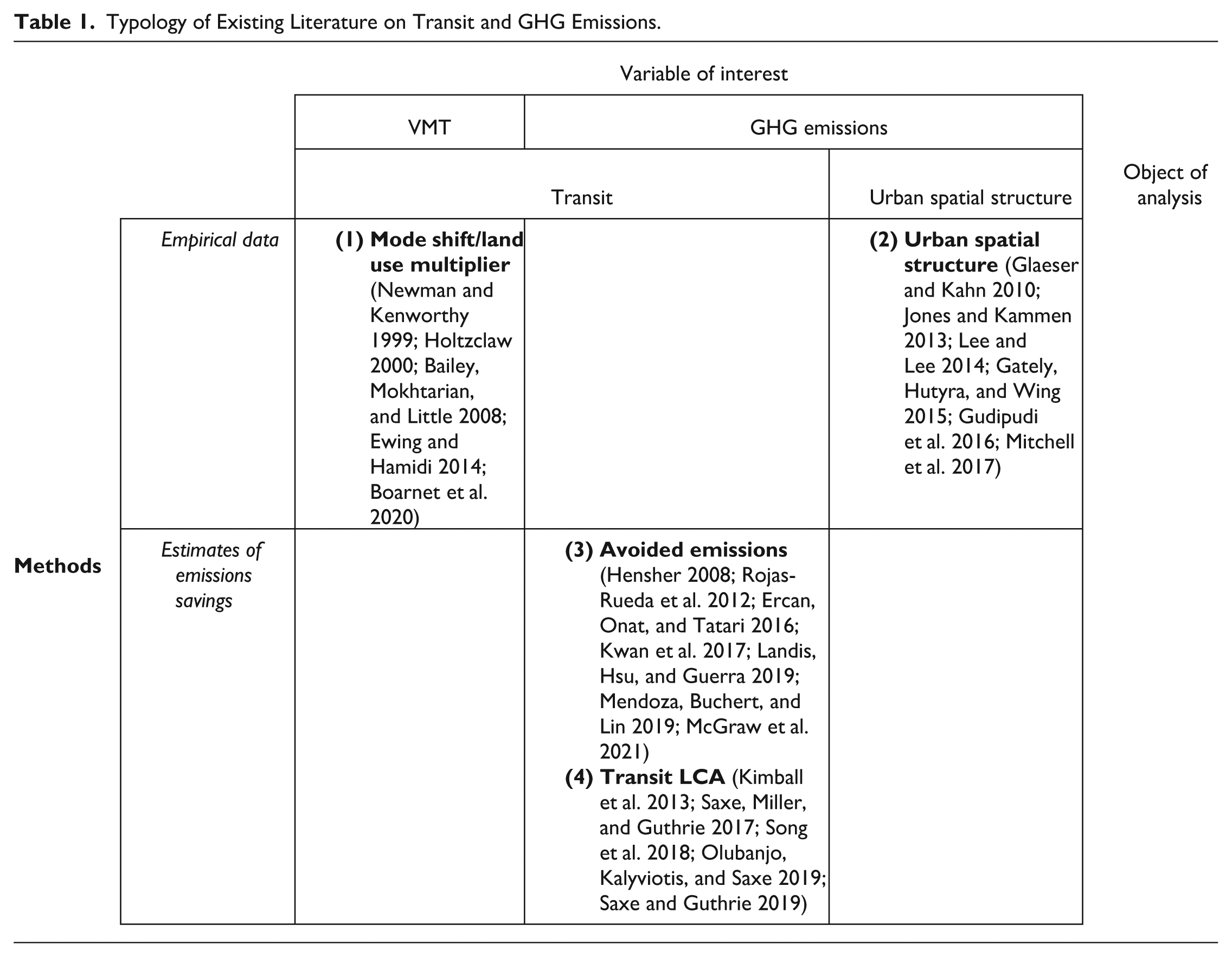
This body of research generally shows that dense, compact central cities have lower emissions per capita than suburban areas (Glaeser and Kahn 2010; Lee and Lee 2014; Mitchell et al. 2017), with some studies revealing a non-linear or “U”-shaped relationship between density and emissions where emissions increase with density and population up to a certain threshold—in larger auto-oriented suburban areas—after which they tend to stabilize or decline in extremely dense central cities with more non-auto travel options (Gately, Hutyra, and Wing 2015; Gudipudi et al. 2016; Jones and Kammen 2013). In addition, density demonstrates a more significant effect for reducing on-road emissions than it does for reducing emissions from buildings, supporting the idea that transportation behavior is the primary mechanism through which compact cities foster reduced GHG emissions (Gudipudi et al. 2016). Thus, this research indicates that compact growth programs must be coupled with modal shifts to attain significant potential reductions in emissions (Landis, Hsu, and Guerra 2019). This aligns with the findings of related empirical research on the impact of transit on travel behavior, which shows that transit construction fosters reductions in VMT not only through direct modal shifts to transit but also through secondary modal shifts (i.e., walking) due to subsequent policy-supported impacts to land use (Bailey, Mokhtarian, and Little 2008; Boarnet et al. 2020; Ewing and Hamidi 2014; Holtzclaw 2000; Newman and Kenworthy 1999).
These conclusions are supported by additional work that generally shows important estimated reductions in GHG emissions due to modal shifts away from private automobiles to lower-emission modes such as transit or walking and biking (Ercan, Onat, and Tatari 2016; Kwan et al. 2017; Landis, Hsu, and Guerra 2019; McGraw et al. 2021; Mendoza, Buchert, and Lin 2019; Rojas-Rueda et al. 2012). In particular, rail transit and associated TOD often provide a favorable emissions benefit to cost ratio (Chatman et al. 2019; Kimball et al. 2013), with some large transit projects able to “pay back” the GHGs involved in their construction within as little as nine to thirteen years (Saxe and Guthrie 2019; Saxe, Miller, and Guthrie 2017).
However, significant questions remain as to the empirical effect of new transit investment on regional CO2 emissions. This paper builds on the existing literature by exploring the relationship between rail transit investment and regional CO2 emissions using a methodological approach that provides a direct estimate of the empirical (rather than projected potential) effect of transit construction on emissions. Unlike LCAs of individual transit projects, however, this paper evaluates a large number (thirteen) of transit systems with an eye toward better understanding the factors that predict success in reducing expected regional CO2 emissions (post-construction). The focus, then, is on understanding the aggregate impact of transit construction for on-road CO2 (and thus indirectly for travel behavior) rather than the direct accounting of specific projects’ emissions costs and benefits.
Data and Methods
Data
The primary dataset used in this study is the Database of Road Transportation Emissions (DARTE), which provides estimates of annual on-road CO2 emissions. While a variety of bottom-up datasets have been used in recent years to model on-road CO2 emissions, including county-level data from the National Mobile Inventory Model (NMIM) County Database (NCD) (Gudipudi et al. 2016), EPA’s newer Motor Vehicle Emission Simulator (MOVES), estimates from the Hestia Project (Gurney et al. 2012; Patarasuk et al. 2016; Rao et al. 2017; Zhou and Gurney 2010), and FIVE (McDonald et al. 2014), DARTE has the advantage of providing coverage for the entire United States at the block group scale for every year from 1980 to 2017, allowing for the kind of quasi-experimental analysis used in this paper.
DARTE uses information from the Federal Highway Administration’s (FHWA) Highway Performance Monitoring System (HPMS) on vehicle miles traveled (VMT) by roadway, along with temporal and state-specific emissions dynamics for multiple types of vehicles and highway classifications at the road segment scale, to create on-road CO2 emissions for every year from 1980 to 2017 at a one-km grid for the continental United States (Gately, Hutyra, and Wing 2019). These estimates are also provided at the Census block group level. The block group data, aggregated to 2010 U.S. Census Core-Based Statistical Area (CBSA) boundaries (U.S. Census Bureau 2003), was divided by yearly population data by CBSA from the Bureau of Economic Analysis (BEA 2018) to create measures of regional on-road CO2 emissions per capita. Due to right-skewness, the natural log of on-road CO2 emissions per capita (
Quasi-Experimental Study Design
Since it is often not ethical to create the conditions for a true controlled randomized experiment in urban planning or social science contexts—and impossible to do using secondary data sources—researchers have developed a set of quasi-experimental methods that simulate the conditions of a randomized experiment using study design and statistical controls (Angrist and Pischke 2015; Cook and Campbell 1979; Imbens and Rubin 2015; Rubin 1974; Rubin 2006; Shadish, Cook, and Campbell 2002). This paper uses a new version of the difference-in-differences (DID) approach known as the “event study” (Athey and Imbens 2018; Autor 2003; Borusyak and Jaravel 2018; Clarke and Schythe 2020; Costa-Ramón2020; Cunningham 2021; Miller, Johnson, and Wherry 2021; Schmidheiny and Siegloch 2023).
The basic logic of the event study is to use data on a panel of observations (in this case, CBSAs) to identify the impact of some intervention or “treatment” (light rail construction) on the post-intervention value of a quantity of interest (on-road CO2 emissions per capita). Identification of the treatment effect comes from comparing the value of the outcome variable in the observations that receive the treatment after the intervention and the counterfactual: observations in which the intervention has not yet occurred or never occurs (the “control” or “comparison” group) (Clarke and Schythe 2020).
Event studies differ from the traditional DID specification in a couple of important ways. First, the time periods before and after around the intervention are normalized for the entire treatment group. This means that data for, e.g., six years prior to treatment is compared evenly across regions, even if that year is 1981 for Portland-Vancouver-Hillsboro, OR-WA vs. 2004 for Phoenix-Mesa-Glendale, AZ. This allows for a clear visual comparison of the pre- and post-intervention values of the outcome variable, which is a key component of the event study’s appeal (Cunningham 2021). Second, event studies decompose the dynamic yearly effects of treatment by creating a series of dummy variables for each year leading up to and following the intervention. In this case, with data for all regions from 1980 to 2017, and interventions spanning 1986 to 2009, the full effect window spans
Formally, quasi-experimental studies should meet three conditions: exchangeability (the provision of the treatment is not related to the likely outcome), positivity (treatment and control areas maintain parallel pre-intervention trends in the outcome variable), and the Stable Unit Treatment Value Assumption (SUTVA) (treatment and control group composition does not change over time and one observation’s outcomes are not affected by the treatment of a neighboring observation) (Matthay et al. 2020; Rubin 1974). In practice (in a planning or policy context), of course, it is not possible to randomly assign the treatment, and there may be systematic differences in the treated and non-treated observations that independently explain changes in the outcome variable (for instance, regions that build new transit systems may be more likely to have residents or policies that favor other types of CO2-reducing behavior compared to regions that do not build transit systems).
To achieve exchangeability, confounding variables (those that cause both the treatment and the outcome) need to be identified and controlled for in the model. The study design should also involve the selection of an appropriate “control” or “comparison” group to minimize systematic unobserved differences between the treated and non-treated observations
2
; as Rubin (2005) explains, the “critical requirement” for estimating a causal effect is that “the comparison must be . . . for a common set of units” (emphasis added) (p. 323). However, in practice, this is difficult to obtain in many urban planning and policy scenarios. Thus, one of the most widely-used methods for controlling for systematic differences between treated and non-treated observations is to include individual year (
Event studies are particularly useful in assessing the validity of the positivity assumption because they visually display the pre-intervention dynamics of the treatment effect. While not a formal test of parallel trends, values of the coefficients of the pre-intervention dummies close to zero provide some evidence that, leading up to the intervention, treated and non-treated observations did not have significantly different values for the outcome variable (Cunningham 2021). In particular, we are concerned with the presence of an “anticipation effect” where the pre-intervention trend appears to be already moving in the direction of the post-intervention estimates. Finally, the DARTE data structure (aggregated from the “bottom up” to a stable areal unit definition, 2010 block groups) and choice of unit of analysis (CBSAs, which are large and discontinuous so as to diminish spillover effects) used in this study satisfy the SUTVA.
Sample and Comparison Group Selection
The broad consideration set for possible treatment regions (i.e., those that built transit within the dataset timeframe) was identified by searching APTA reports to compile a list of CBSA-specific years in which each continental U.S. region’s first rail transit system opened 3 (2019), shown in Table 2. In this case, six years was selected as the minimum required pre- or post-construction runway, so Portland-Vancouver-Hillsboro, OR, with its 1986 construction of the MAX light rail system, was chosen as the first region to analyze. Additionally, only light rail systems of sufficient length (i.e., more than ten miles) were selected, which precludes Tampa’s TECO streetcar, Memphis’ MATA trolley, and Norfolk’s The Tide light rail from inclusion within the 2011 post-construction cutoff, as well as newer streetcar systems in Tucson, Kansas City, Cincinnati, and Detroit. This leaves thirteen regions for analysis, which amounts to some 38 percent of the regions in the continental United States that have ever built any kind of rail transit system (through 2017), a significant sample for analysis.
List of U.S. Rail Transit System Openings by First Year in CBSA.
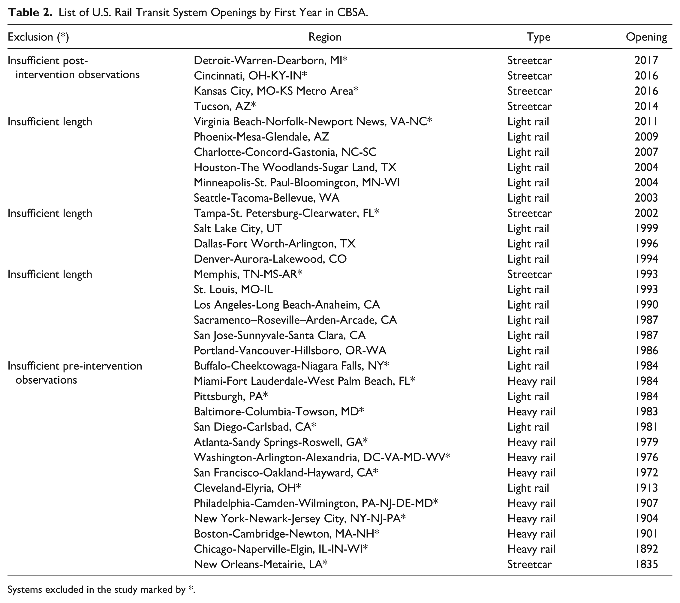
Systems excluded in the study marked by *.
With the sample selected, the next task was to select an appropriate comparison group. As mentioned earlier, in quasi-experimental studies, the “control” or “comparison” group should ideally be as similar to the treatment group in every regard other than that the treatment group received the treatment, so that any deviation in the outcome variable between the treatment and control areas after the treatment occurred can be attributed to the treatment itself (Rosenbaum and Rubin 1983; Rubin 2006; Stuart et al. 2014).
However, given the significant differences between the thirteen regions that built transit in our sample and those that did not, any choice of comparison group comes with unavoidable shortcomings that must be acknowledged as an inherent limitation of the paper’s approach. In the absence of an a priori choice of comparison, this paper’s primary specification uses a comparison group defined empirically using propensity score matching. The basic idea of this technique is to build a logistic regression (using covariates from the first year of the study, i.e., 1980) that predicts whether or not a region eventually builds light rail. Based on similarity in the predicted values from that model (the “propensity scores”), each treated region is then matched 4 to one 5 of the remaining 340 non-treated regions.
Following the methodology of Ho et al. (2007, 2011), propensity scores were calculated for the full sample of non-excluded (353) CBSAs using the “MatchIt” package in R v.4.0.4. The propensity scores here are based on available predictors of public transport construction at the regional level from the 1980 Census: percent commuters who use transit, population density, percent of workers working in the central city of the region (as a proxy for employment density), and the weighted average number of vehicles per household. These specific variables were chosen based on conceptual similarity to previously-identified predictors of light rail ridership (Currie, Ahern, and Delbosc 2011). While there is not much existing research on predictors of regional propensity to construct light rail, transit service levels, car ownership rates, population density, and employment density have been identified as important factors for predicting light rail usage. 6 The full diagnostics for the propensity score estimation, as well as a list of the matched treatment-comparison pairs, can be found in Supplemental Appendix A.1.
To ascertain the robustness of this choice, we have also run several additional models—described in Supplemental Appendix A.2—with alternative definitions of the comparison group, including (1) no comparison group; (2) choosing only the regions that built transit later in the period (2007-2017) as the comparison group, tested against those which built transit earlier (1986-1996); and (3) a comparison group that contains all 340 never-treated CBSAs. Supplemental Appendix A.2 also includes results for a model based on the propensity score comparison group with region-specific time trends included and the table of coefficient values for all specifications.
Model Specification
The general panel event study specification is shown in equation (1) (Clark and Schythe 2020; Cunningham 2021):
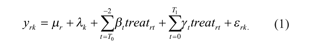
where:
The simple intuition of the event study approach is that it creates individual dummies for each year leading up to and lagging after the intervention (other than
It is important to note that, as Cunningham (2021) explains: “any DD [difference-in-differences] is a combination of a comparison between the treatment and the never treated, an early treated compared to a late treated, and a late treated compared to an early treated.” In a staggered adoption event study, where interventions occur at different times for different observations (as is the case in this paper), a large body of recent work has identified that the TWFE estimator is unbiased only if the treatment effect is constant between units and over time. This is primarily due to the implicit comparison of treated units in “treated” time periods to other treated units in “untreated” time periods in binary treatment staggered adoption TWFE models (Callaway and Sant’Anna 2021; de Chaisemartin and D’Haultfœuille 2023; Goodman-Bacon2021; Sun and Abraham 2020).
Thus, in this paper, we use the event study estimator developed by de Chaisemartin and D’Haultfœuille (2024) and implemented in the “DIDmultiplegtDYN” package in R (de Chaisemartin et al. 2025). Essentially, the de Chaisemartin and D’Haultfœuille (2024) estimator constructs comparisons between regions (groups) with the same treatment status in time period one for the periods before they “switch” into treatment, which avoids the contamination from using already-treated units as counterfactuals. The DID estimator in post-intervention time period
Results and Discussion
The graph of the event study placebos and effects is shown in Figure 1, with matching statistical results provided in Supplemental Appendix A.2.1. In terms of satisfying the parallel trends and “no anticipation” assumptions, none of the placebos are statistically significantly different than 0, and the visual pattern of pre-intervention differences between treatment and comparison groups in Figure 1 is very flat, as desired. However, the formal test of placebo nullity is rejected, suggesting that there may be some small systematic differences in pre-intervention trends between the treatment and comparison groups.
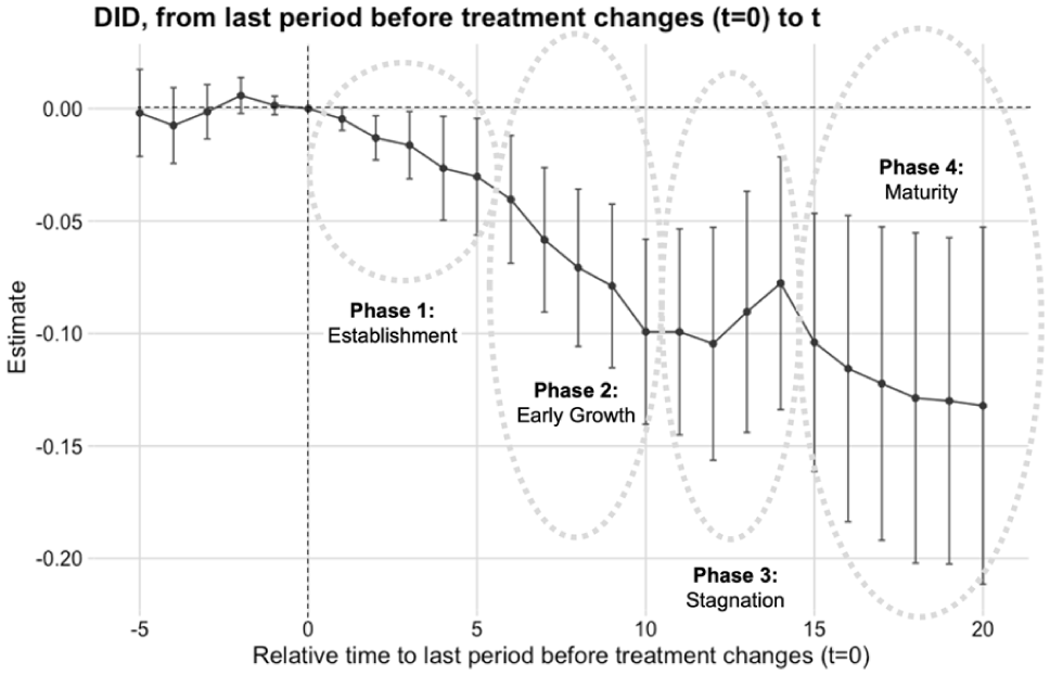
Graph of the event study results using the de Chaisemartin and D’Haultfœuille (2024) estimator on the dependent variable
As Figure 1 indicates, the effect of light rail construction on reducing
What does this mean in a planning context? Broadly, the results indicate that light rail construction has a statistically-significant effect on reducing regional on-road CO2 per capita, but (most importantly) the nature of this effect changes over time. In Figure 1, the empirical effects from the model have also been qualitatively grouped into four distinct “eras” or phases of light rail effect, each about five years long, which chart the long-term evolutionary dynamics of system operation. In the first phase (Establishment), systems are just beginning services, and substantial reductions in regional on-road CO2 (i.e., reductions in driving) are not observed: it takes some time for residents and businesses to adapt to the presence of a new transportation system and integrate its use into everyday routines.
Importantly, this analysis cannot separate the effect of light rail construction on reduced CO2 that is due to (1) changes in land use, (2) changes in walking behavior, and (3) changes in transit behavior as in other studies (Ewing and Hamidi 2014). All three of these regional processes are captured by the average effect produced by the model in a given year, and certainly we would expect transit-oriented land use changes to be long-run investments that take many years to be implemented. In addition, it is likely that treatment intensity and/or effectiveness (which this analysis does not capture) generally increases over time as lines are expanded, new stations are constructed, service is increased, and so on. All of this helps explain why the initial five-year period does not show very large magnitudes for the impact of light rail construction.
However, starting in year six, the second phase (Early Growth) begins to exhibit larger magnitudes in light rail effects. This is likely due to increases in ridership as some of the short- and middle-run changes in behavior patterns and business establishment begin. For example, previous research showing significant increases in new businesses starts near light rail lines within six years after construction (Credit 2018), which matches the time horizon of “early growth” indicated by the results here.
Interestingly, though, after 10 years of system operation, the results suggest that new systems enter a phase of “stagnation” with flattening impacts to CO2 reduction. This plateauing effectiveness is likely due to the well-identified “novelty factor” for new public transport systems (Mohammad et al. 2013). As Credit (2018) explains, based on the findings of previous research: “there appears to be a much higher anticipated value or perceived benefit to a new rail transit system that catalyses economic activity leading up to, or shortly following, its opening, which then dissipates as the ‘novelty factor’ wears off.” In fact, data on raw light rail system ridership (available starting in 2002) for systems that opened between 2002 and 2009—which includes Seattle-Tacoma-Bellevue, WA, Houston-The Woodlands-Sugar Land, TX, Minneapolis-St. Paul-Bloomington, MN-WI, Charlotte-Concord-Gastonia, NC-SC, and Phoenix-Mesa-Glendale, AZ—shown in Figure 2 demonstrates a clear “plateau” or stagnation period after an initial growth phase for each system (depending on how the break in trend is defined, etc.) (NTD 2025).
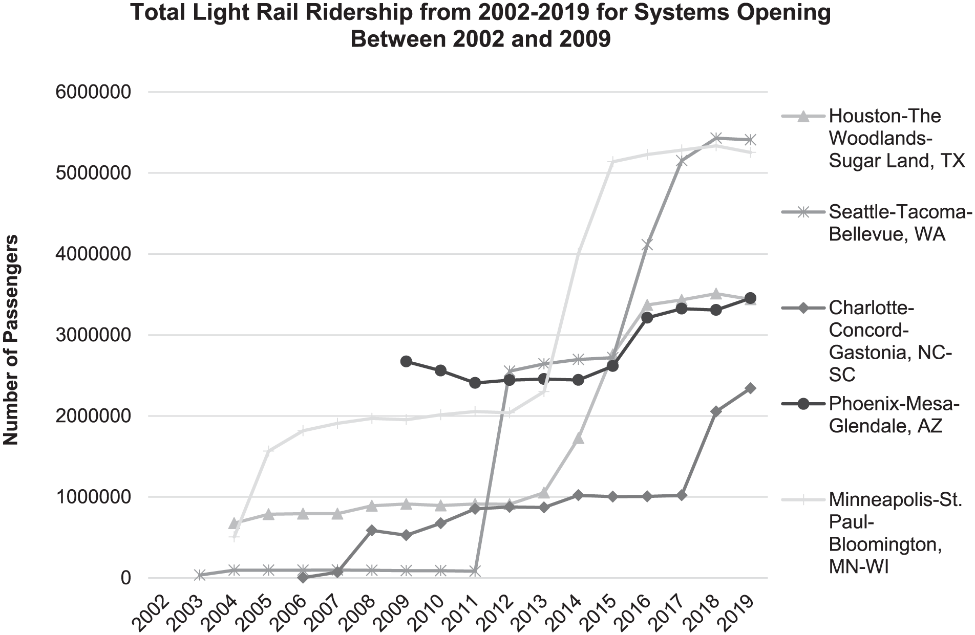
Graph showing raw light rail ridership from 2002 to 2019 for five light rail systems in this study’s sample that opened within this timeframe (NTD 2025).
Finally, as systems emerge from the “valley of death” in the stagnation phase in year fifteen and enter operational “Maturity” (Phase 4), the estimated impacts increase once again. While this is likely due to the realization of long-term investments and increases in service effectiveness and delivery described above, it is important to note that the model’s estimates here come with a larger amount of uncertainty as well. Overall, the average cumulative (total) effect per treatment unit 9 is −0.070 (shown in Supplemental Appendix A.2.1), indicating that on average (across all years of operation in all treated regions) light rail construction resulted in a 6.8 percent (exponentiated) reduction in on-road CO2 emissions per capita.
In general, the finding of a significant long-run effect for light rail construction is useful for planners tasked with evaluating the long-range impacts of infrastructure investment decisions. It is also important for researchers to note that this dynamic effect would not be apparent without the use of the event study approach, as the traditional DID estimator bundles all of the dynamic post-intervention effects together into one coefficient value. However, these results come with a few limitations, which are important to highlight in detail. First, it is critical for the reader to understand that while the general pattern of results presented here are robust to modeling choices (as shown in Supplemental Appendix A.2), the selection of estimator, specification, comparison group, number of placebos and effects, etc., all have demonstrable impacts on the point estimates produced by any given model. In other words, while event studies are primarily intended to show significant causal effects and fit with the parallel trends assumption, any specific point estimate should be taken with a grain of salt. This is also true for the overall average estimated treatment effect (6.8%), which is larger than estimates from previous work on the overall impact of light rail construction on VMT reduction (e.g., 2.9%—see Supplemental Appendix A.4) (Ewing and Hamidi 2014).
The variation in point estimates is partially due to the difficulty in fulfilling all of the assumptions of quasi-experimental study design (particularly exchangeability) in the context of this paper’s research question. It is not possible to find a perfectly well-matched comparison group for regions that built light rail, which means that any estimates rely on the two-way fixed effects to adjust for differences between treated and control observations, which is always imperfect. This also means that there may be some systematic differences in pre-intervention trends between the treatment and comparison groups.
In addition, there is significant heterogeneity in the raw temporal pattern of the dependent variable (and likely the treatment effects) for individual regions, which may result in an “average” effect reported by the model that is simply a numerical middle-ground between very effective and very ineffective regions; unfortunately, we cannot assess these heterogeneities using the methodological approach and data available here. Similarly, we are not able to account for treatment intensity or effectiveness (i.e., system length or service quality) which may be driving (unobserved) heterogeneities in the result. Given the very long time span of the study, regions that built systems earlier may be fundamentally different than those that built systems later; newer systems may be better designed or planned than older ones (or vice-versa). Finally, the overall effects of light rail construction on CO2 emissions (and thus driving) estimated here cannot be separated by the portion that is due to changes in land use, changes in walking behavior, or changes in transit ridership. While other studies have shown that the impact of light rail on increasing walking may be responsible for the biggest reductions in driving (Ewing and Hamidi 2014), the larger magnitude of long-run estimates (e.g., from about year fifteen to twenty) in this paper suggests that land-use adaptation and change might be even more important; this question should be assessed further in future research.
Conclusion
While a wealth of existing research has identified the potential effectiveness of reducing transportation-related CO2 through increased usage of non-auto modes (Chatman et al. 2019; Ercan, Onat, and Tatari 2016; Gudipudi et al. 2016; Kimball et al. 2013; Kwan et al. 2017; Landis, Hsu, and Guerra 2019; McGraw et al. 2021; Mendoza, Buchert, and Lin 2019; Olubanjo, Kalyviotis, and Saxe 2019; Rojas-Rueda et al. 2012; Saxe and Guthrie 2019; Saxe, Miller, and Guthrie 2017; Song et al. 2018), to the author’s knowledge, there are no existing studies that analyze the aggregate effectiveness of transit investment at the regional scale across a twenty-five-year period using causal analysis. This knowledge is particularly important for planners pursuing transit investment in new regions, which are often justified (at least in part) based on their environmental benefits. By employing a quasi-experimental methodology that uses a cutting-edge event study estimator to analyze the impact of building a light rail system on reducing on-road CO2 emissions per capita, this paper provides an initial understanding of the causal role that light rail system construction has on regional transportation behavior. The results indicate that light rail construction has a significant impact on reducing regional CO2 emissions per capita, and that these effects change dynamically for at least twenty years after construction. The paper categorizes these long-run effects into four phases of light rail operational effectiveness, each about five years long: (1) establishment (negligible initial effect on CO2), (2) early growth (increasing magnitude of effect), (3) stagnation (plateauing effect), and (4) maturity (renewed, high magnitude effects on CO2 reduction). While the generalizability of these trends needs to be investigated in future work, these results provide a useful framework for studying and thinking about the long-run operational dynamics of public transit systems.
From the standpoint of planning practice, the results show that transit’s effect on
At the same time, the primary limitation of this approach is related to sample size and comparability—even over a thirty-seven-year period, the number of regions that built transit systems is relatively small, and there are systematic differences between the regions that built and did not build transit systems that are hard to truly eliminate in this study. While regional impacts remain important to understand, future work leveraging the fine-grained scale of the DARTE dataset at the block group level to create targeted, intraurban treatment and control areas may be able to overcome some of these sample size issues while at the same time providing estimates of the heterogenous effects of transit construction on carbon emissions within regions. Further analysis of the features of both the regions and the transit systems themselves that relate to significant reductions in on-road emissions is also needed in the future to provide planners with concrete insights on supportive policies for achieving larger transportation-related reductions in GHGs. Despite these limitations, the results of this paper provide planners and policy-makers with an important empirical understanding, using a novel methodology, of the aggregate effect of light rail construction on reducing regional on-road CO2 emissions.
Supplemental Material
sj-csv-2-jpe-10.1177_0739456X251396878 – Supplemental material for The Long-Run Dynamic Impact of Light Rail Construction on Regional On-Road CO2 Emissions per Capita
Supplemental material, sj-csv-2-jpe-10.1177_0739456X251396878 for The Long-Run Dynamic Impact of Light Rail Construction on Regional On-Road CO2 Emissions per Capita by Kevin Credit in Journal of Planning Education and Research
Supplemental Material
sj-docx-1-jpe-10.1177_0739456X251396878 – Supplemental material for The Long-Run Dynamic Impact of Light Rail Construction on Regional On-Road CO2 Emissions per Capita
Supplemental material, sj-docx-1-jpe-10.1177_0739456X251396878 for The Long-Run Dynamic Impact of Light Rail Construction on Regional On-Road CO2 Emissions per Capita by Kevin Credit in Journal of Planning Education and Research
Footnotes
Acknowledgements
I am grateful to the anonymous reviewers for their constructive comments and thoughtful suggestions, which significantly improved the quality of this manuscript. I would also like to thank Dr. Orsa Kekezi for her valuable assistance and insights during the revision process.
Declaration of Conflicting Interests
The author declared no potential conflicts of interest with respect to the research, authorship, and/or publication of this article.
Funding
The author received no financial support for the research, authorship, and/or publication of this article.
Supplemental Material
Supplemental material for this article is available online.
Notes
Author Biography
References
Supplementary Material
Please find the following supplemental material available below.
For Open Access articles published under a Creative Commons License, all supplemental material carries the same license as the article it is associated with.
For non-Open Access articles published, all supplemental material carries a non-exclusive license, and permission requests for re-use of supplemental material or any part of supplemental material shall be sent directly to the copyright owner as specified in the copyright notice associated with the article.