
Abstract
The discovery of power laws in conflict intensities has spurred numerous explanation attempts. Two different interpretations have persisted: the notion that power laws are spurious results of random processes and the opposing view that power-law distributions attest to endogenous dynamics linked to self-organized criticality (SOC). We substantiate the SOC forest-fire model for intrastate conflicts, conceptualizing conflict potential as social pressure, measured by horizontal inequality. This potential is triggered by infinitesimal events. Their occurrence depends on the interaction density between conflict actors, operationalized as the conjunction of state capacity and non-state governance. In a global analysis of 143 conflict dyads, we find that 40 conform to a power law and 33 to a stretched exponential distribution, the two outcomes predicted by the model. We find evidence that the forest-fire model is a plausible approximation of the dynamics of intrastate conflicts, accounting for both the conformity and the non-conformity to power laws.
Keywords
Introduction
This article addresses an “enduring mystery” in the study of conflict: the existence and meaning of power laws (Clauset 2020). The mystery persists especially with regard to the intensity dynamics of intrastate conflicts between governments and non-state actors. Power laws (PLs) in conflict dynamics and their impact on growth processes such as escalation have been known ever since the research of Lewis Richardson (1948)—mathematician, physicist, meteorologist, and one of the founders of quantitative conflict research. While PLs are associated with pivotal characteristics that shape the severity and predictability of outbursts of violence, their importance for conflict research has rarely been recognized (Cederman 2003; Cederman et al. 2011a). A fundamental reason for this is that the origins of PLs in general and in armed conflicts in particular are far from understood. Two rival explanations have been put forward: while skeptics state that PLs are spurious results of random processes, the opposing view of complexity science argues that PL distributions attest to endogenous dynamics linked to self-organized criticality (SOC). This question is related to how conflict dynamics are understood. While proponents of the former stance tend to prefer stochastic models that emphasize hierarchical control in rebel organizations, the latter perspective stresses the role of endogenous, spontaneous mass dynamics.
This article seeks to shed light on the plausibility and validity of the SOC paradigm by empirically substantiating and testing the so-called forest-fire model as one of the most widely known complexity models of generating PL distributed data (Drossel and Schwabl 1992). The model posits self-propagating cascade effects as the central mechanism of escalation dynamics. It suggests two parameters: an accumulating action potential and an activation parameter, the latter taking the form of intermittent sparking events that trigger avalanching activities propagating through the network. When applied to intrastate conflicts, each avalanche of a given size represents a conflict event of a certain intensity. The key aspect of the forest-fire model is that it predicts two alternative empirical distributions depending on the activation parameter configuration: a PL decay and an exponential deviation. Among other characteristics, the two types diverge with regard to how “big” a conflict might become, with conflicts obeying a PL being more likely to attain extreme event sizes than conflicts following an exponential distribution. We take advantage of this dual prediction feature of the model to assess its value based on conflict event data. If both distributions appear in the data and if they are each associated with the predicted manifestation of the parameters, this speaks in favour of the forest-fire model. This in turn lends support to the idea that SOC models with their emphasis on non-linear dynamics are serious rivals to stochastic models, which tend to underestimate the consequences of social complexity on conflict processes.
This article has both a theoretical and an empirical focus. Section 2 gives a short overview of important characteristics of PLs and the relevant state of research in conflict studies. Section 3 assesses the general plausibility of the SOC paradigm, introduces the forest-fire model, and derives testable hypotheses from it. Section 4 measures the dependent variable by providing a rigorous global analysis of the distribution of conflict event intensities between 1989 and 2020, operationalizes crucial variables derived from the model, and tests the hypotheses empirically. Given the exploratory stage of the research on intensity distribution types and the limited number of cases in our sample, we turn to a systematic evaluation of binary classifiers as our method of choice. The article concludes with a discussion of the implications of our findings.
Power laws in conflict research
The following gives a quick primer on the characteristics of PLs. PL distributions are highly right-skewed: they have a “fat” or “thick tail”, i.e. large events are much more common than is to be expected under a normal distribution (Newman 2005). Data that obey a PL have no typical value around which to fluctuate (Bak 1996): they are scale-invariant, which means there is no fundamental difference between small and large events (Clauset et al. 2007). Large events are simply bigger variants of smaller events. There is therefore no reason to assume different data-generating mechanisms for large and small events. All events in a PL distribution are generated by a common mechanism, bringing forth incidents of varying magnitude. This points to the possibility of some “deep structure” underlying various forms of political conflict, from strikes and protests to terrorist attacks and massacres to insurgencies and civil wars (Spagat et al. 2018).
The practical importance of PLs lies in the chances and limits of predictability they hold out. PL distributed data show a characteristic blend of randomness and regularity. The frequency y of an event of a given size obeys a PL if it is inversely dependent on the event size x:
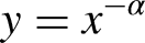
Illustrating the scale invariance (left) and burstiness (right) of power-law distributions.
The remarkable regularity appearing in log–log plots is absent in the time series of PL distributed events, which is distinguished by a characteristic burstiness (Bohorquez et al. 2009): the sequence of many small and a few medium-sized events is interrupted by a limited number of extremely large events (Figure 1, right). The size range potentially stretches across several orders of magnitude. In bursty time series, there is no periodic pattern of recurrence and no apparent escalatory build-up in intensity. An extreme event might be imminent without warning. Owing to this characteristic, under PLs there is no way to predict when an event of a certain size will occur—if it will occur at all. It is this unpredictability of the timing of extreme events that makes PL phenomena so worrisome (Brunk 2002; Taleb 2007).
In only few empirical cases does the data follow one distribution over the whole value range. Most of the time, the theoretical distribution can only be identified above some lower bound xmin and below some upper bound xmax. In the context of conflicts, a possible reason for the existence of a lower bound is the poor data coverage at low intensity levels: if small events are not reported as rigorously as large events, their relative frequency will be understated in the data, distorting the fitting of the distribution (Friedman 2015). Upper bounds, known as “exponential cutoffs”, owe their occurrence to the fact that, while under conditions of scale invariance events of any size are conceivable in principle, this is subject to empirical restraints: there is simply not enough energy that can be emitted to generate events of extreme orders of magnitude (Farmer and Geanakoplos 2008). This is called the “finite-size effect” (Bak et al. 1987; Newman 2005).
PLs are ubiquitous in the natural and social world, covering phenomena as diverse as word frequencies, city sizes, book sales, stock-market crashes, earthquakes, and forest fires (Turcotte 1999; Newman 2005; Clauset et al. 2009; Tenreiro Machado et al. 2015). There is increasing evidence that the distributions of the intensities of many forms of political conflict in the past centuries fit a PL distribution (Hegre et al. 2017; Spagat et al. 2018), including interstate wars (Richardson 1960; Levy and Morgan 1984; Cioffi-Revilla 1991; Roberts and Turcotte 1998; Cederman 2003; Cioffi-Revilla and Midlarsky 2004; Clauset 2018, Cunen et al. 2020), intrastate armed conflicts (Gulden 2002; Cioffi-Revilla and Midlarsky 2004; Lacina 2006; Friedman 2015; Trinn 2015; Lee et al. 2020), terrorist attacks (Alvarez-Ramirez et al. 2007; Clauset et al. 2007; Clauset and Wiegel 2010; Johnson et al. 2011; Pinto et al. 2012; Clauset and Woodard 2013), one-sided violence against civilians (Bohorquez et al. 2009; Scharpf et al. 2014), strikes (Biggs 2005; Campolieti 2019) and protest activity on social media (Zhukov et al. 2020).
Despite the consistent empirical findings, the theoretical debate on what might explain PL distributions in conflict intensities is far from being settled. The research community is essentially divided over the role of complexity vs. randomness in generating PL distributed data. On the one side we find the assertion that PLs “are simply statistical phenomena, that is, spurious facts” (Pinto et al. 2012: 3559; see Touboul and Destexhe 2010). In this view, PL distributions are generated by “stochastic processes, in which noise is supplied by an external source and then amplified and filtered” (Farmer and Geanakoplos 2008: 43; see Clauset et al. 2007). The primary “motor” in such stochastic models is exogeneous random fluctuations processed by simple mathematical operations. According to this view, there is no diagnostic value in the occurrence of PL distributions. They are just chance phenomena which can be arrived at via various routes (Sornette 2009). Precisely the fact that PL distributed data are so ubiquitous is seen as evidence that they are produced by ubiquitous, and essentially meaningless, noise.
Stochastic models heavily rely on fine-tuning. Clauset and Young (2005) and Clauset et al. (2007), for instance, use a “killed exponential growth” process to generate PL-distributed sizes of terrorist attacks. The authors assume that the potential severity of an attack increases exponentially with the time t invested in its planning (e κt ). They further argue that some of the potential attacks are prevented or aborted. The likelihood of a successful execution is assumed to be inversely exponentially related to its potential severity (e−λt). The parameters κ and −λ are constants. The value of the PL exponent α equals 1 − (κ/−λ). Under this model, a PL only emerges if the “mixed” variables are both exponentially distributed.
Johnson et al. (2006) and Bohorquez et al. (2009) study the size distribution of conflict events in insurgencies. Their iterative model consists of (non-interacting) “attack units”, i.e. conglomerates of resources. With a probability v, a randomly chosen attack unit either fragments into several units or merges with another unit with probability 1 − v. A fragmenting unit of strength s disintegrates into s new units. The likelihood that an attack unit is selected is proportional to its strength, i.e. stronger units are assumed to be under greater pressure and more likely to fragment or coalesce. There is a total amount of attack strength in the model, i.e. a closed pool consisting of all resources available to the insurgents, which is, in effect, continually re-distributed among attack units. The severity of an event is assumed to be linearly equivalent to the perpetrator unit's strength, i.e. to the resources available to it at a given time. Overall, the event intensities follow a PL.
Fine-tuning is noticeable in the double exponential function requirement in the model by Clauset et al. (2007). In the model developed by Bohorquez et al. (2009), fine-tuning finds expression in the requirement that attack units completely disintegrate into a number of equally sized and non-divisible entities. This concept is too vague and too specific at the same time. It is inconceivable which social phenomenon should correspond to these entities. The viability of the models wholly depends on whether these requirements are precisely met. That this is the case is questionable, casting doubt on the plausibility of these models.
The plausibility also suffers from issues closer to the topic of political conflict. The discussed approaches reduce the interactive dynamics of political conflicts to processes internal to collective actors. There is no interaction taking place between the model entities. Event sizes are simply assumed to be equivalent to actor-centric circumstances such as the time required to plan an attack or the perpetrator's resources. There is no conflict dynamic from which the outcome, the PL distribution of conflict intensities, could emerge.
On the other side of the theoretical divide, we find SOC models with iterative interactions between entities, where within-network dynamics are given causal priority over chance (Hergarten 2002). The system's current state arises from internal processes, i.e. it is more determined by its own preceding states than by exogenous input (Braha 2012). SOC models also amplify noise provided by an external source, but the amplification is potentially infinite, so that even an infinitesimal noise source is amplified to macroscopic proportions. In this case the properties of the resulting noise are independent of the noise source, and are purely properties of the dynamics. (Farmer and Geanakoplos 2008: 43)
The researchers who rediscovered Richardson's law for conflict studies at the turn of the twenty-first century (Roberts and Turcotte 1998; Cederman 2003) favourably discussed the “forest-fire model”, which belongs to the family of SOC models. Later on, however, quantitative conflict research tended towards a variety of stochastic explanations (Clauset et al. 2007; Bohorquez et al. 2009; Cederman et al. 2011a). This has, perhaps, much to do with the fact that it is difficult to reconcile the superindividual dynamics of the complexity paradigm with the actor-centered theories prevalent in contemporary conflict studies. In comparison, stochastic approaches with their mathematical bareness appear to be theoretically less invasive.
Difficulties for the complexity paradigm in conflict studies also arise because of the fact that the concepts of SOC are often underspecified for the social world. To make complexity models work in the context of intrastate conflicts, many of their elements must be substantially adapted to the realities of political violence.
The picture becomes even more complex when we take into account that, as noted above, empirically not all natural and social phenomena—and among them not all conflicts—fit a PL distribution (Clauset et al. 2009). Conflict studies have so far largely neglected this issue. Scharpf et al. (2014), for instance, note that about half the conflict settings in their global analysis do not conform to a PL, but they discuss neither the nature of this non-conformity nor its repercussions on the explanation of conflict escalation. Empirical research is required that systematically discriminates between conflicts which conform to a PL and those that do not.
The following section gives an outline of the SOC paradigm and introduces the forest-fire model. We then discuss the concepts of social pressure and grievances, on the one hand, and triggering events and social interaction density, on the other, to substantiate the model in the context of social conflicts. The section ends with hypotheses derived from the substantiated model.
SOC in conflict studies
SOC models are very different from their stochastic cousins. Most of these models are “cellular automata”, i.e. simulations consisting of virtual populations of a large number of individual, discrete grid cells interacting with each other. This is suited to reflecting the distinctive network character of social systems: individuals interact, and from these interactions complex behavioral dynamics emerge from the bottom up (Archer 1995). This includes the processes of intrastate violence, which is, as Kalyvas (2007) and Cederman and Vogt (2017) note, a deeply and inherently endogenous phenomenon. Conflict is a form of spontaneous order. The critical state in SOC systems is self-organized in the sense that the network in question evolves toward this state in a spontaneous manner, without external intervention: the system tends to a state of crisis all by itself.
Crisis is a robust, ubiquitous state in the social world: “The ‘normal’ state of nature is thus not one of balance and repose; the normal state is to be recovering from the last disaster” (Urry 2005: 6). The “disasters” in social systems can be of virtually any size. In SOC models, each disruption is composed of a chain reaction, cascade, or avalanche propagating through the spatial, temporal, and intensity state space. Some of these avalanches simply stop much later than others. Each event cascade is sparked by an infinitesimal incident. This reflects the disruptive nature of social dynamics, where seemingly insignificant triggering events can set off catastrophic avalanches. A prominent example is the Tunisian street vendor, Mohamed Bouazizi, whose self-immolation sparked the 2011 Tunisian Revolution.
In sum, SOC models are plausible representations of the social world since they reflect important features of social dynamics, including political conflict processes. Specifically, they address three issues of complexity: the interdependencies in social networks and the emergent nature of social dynamics; the fact that societies spontaneously return to a state of crisis; and the observation that social systems are characterized by bursts of disruptions that are triggered by infinitesimal incidents. On this general level of consideration, the SOC framework therefore appears to fit well to empirical conflict dynamics.
Mechanics of the forest-fire model
The first SOC model was the so-called “sandpile model” developed by Bak et al. (1987). It consists of a cellular automaton defined on a rectangular grid. At each time step, a grain of sand is placed on a randomly chosen cell. The trickle of sand is the driving force p. Since the factor is small, the dynamic driven by it is slow. The crucial part of the process emerges from the dynamics between the interconnected cells. Grains in a cell are stacked. At a critical threshold of θ = 4, the stack topples and the four grains are distributed to the four neighboring cells. This redistribution effect can propagate across several cells, leading to cascades of PL distributed sizes (Turcotte 1999; Hergarten 2002). The sandpile model generates PL distributions with a constant exponent at α = 0.98. This contradicts the fact that α varies empirically, giving rise to variations in the slope of the PL line. They reflect important differences in the maximally attainable event sizes—in the overall severity of a conflict, for instance. To account for this, Olami et al. (1992) developed the “earthquake model” that generates distributions with varying values of α.
As we discussed above, however, even more substantial deviations from a PL appear in empirical data. To account for such deviations, Drossel and Schwabl (1992) developed the so-called forest-fire model, which generates data distributions with either a power-law or an exponential decay. To the best of our knowledge, the geologists Roberts and Turcotte were the first to apply this model to the distribution of conflict intensities (Roberts and Turcotte 1998; see Lee et al. 2020). The model has two parameters: the parameter p indicates the likelihood that a tree is planted in an empty cell. The parameter f represents the probability with which lightning strikes a cell. If it is occupied by a tree, it will catch fire. The fire then spreads to those neighbouring cells that are occupied by a tree. The resulting cascade of propagating events can be of varying size, depending on the number of available contiguous trees. They may affect one or several cells or even engulf the entire grid.
The lower the probability f that lightning sets a tree on fire, the larger will be the clusters of trees over the course of time, and the larger are the fires that occur if such a forest is eventually ignited. A higher chance that lightning strikes means that trees burn down more frequently and that the clusters of regrowing trees are therefore smaller, as are the fires that break out if the forests are set alight. Thus, under constant tree growth, frequent lightning strikes result in a smaller probability of large fires, and vice versa. Similarly, a higher probability of tree growth increases the size of tree clusters and is thus, ceteris paribus, associated with larger forest fires.
If the ratio of f/p is approaching zero, the system is in a steady critical state. The severity of the fires follows a PL (Drossel 1996). At a higher ratio, with f/p → ∞, the system is in a subcritical state. The dynamic is curbed and drops off, resulting in a transition to an exponential decay over the entire distribution (Hergarten and Krenn 2011; Sachs et al. 2012). As far as conflicts are concerned, an exponential decay points to escalation dynamics that peter out before conflicts can widen into large political conflagrations. It is important to note that under the forest-fire model the existence of distributions deviating from the PL does not diminish the power of the SOC paradigm. On the contrary, subcritical states are as much the result of SOC processes as critical states are.
We can further specify our expectation regarding the empirical occurrence of the exponential decay. Clauset et al. (2009) in their seminal article ruled out the pure exponential distribution for almost all cases. However, they found the stretched exponential (SE) distribution to be a strong competitor of the PL hypothesis, including international and civil wars and terrorism. While the authors did not reach a definite conclusion in this regard, the available evidence suggests that we should be prepared to observe SE distributions (and not pure exponentials) when an exponential decay is theoretically implied.
Closing the gap between model and reality
While finding the forest-fire model suggestive, Cederman (2003) contends that the analogy between wars and wildfires carries not enough explanatory weight owing to the substantial differences between forests and states. This criticism confuses the concepts of analogy and homology, however. The identification of fire cascades with conflict cascades is not based on superficial similarities but on isomorphisms, i.e. on fundamental principles shared by superficially dissimilar systems (von Bertalanffy et al. 1977). While analogical association would lead to metaphorical language, which should be avoided in a scientific context, homological inference rests on the notion of functional equivalence, which is of a high analytical value. The forest-fire model makes a minimal number of assumptions. It is not realistic in the sense of capturing all empirical factors and mechanisms, nor does it seek to establish one-to-one correspondences with the real world. However, it can be used as a starting point for developing more realistic models (Zinck et al. 2010). The specific plausibility of the model, which would add to the general plausibility of the SOC paradigm as discussed above, depends on how well the parameters fit the phenomenon conceptually. As the forest-fire model does not specify the parameters f and p for a social context in general or for intrastate conflicts in particular, it is obvious that this requires a stringent sociological substantiation of the model.
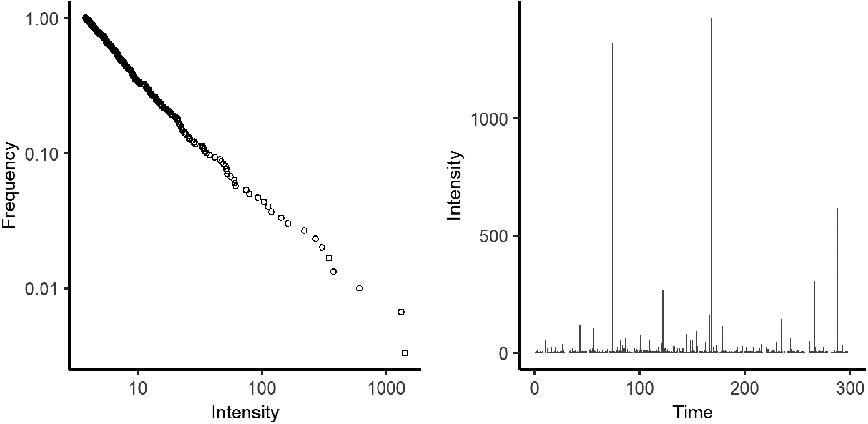
In the forest-fire model, according to the parameter p (the likelihood of “planting trees”), a quantity W (the “forest”) slowly accumulates within the system and is eventually “burned”. In a process specified by the activation parameter f (the probability of “lightning”) random triggers T occur which set off cascades of “fire” C (see Figure 2). These avalanching events are the output of the system.
Theoretical mechanism of the forest-fire model.
If we accept this conceptualization of conflict dynamics, the question arises as to how the variables p and W as well as f and T manifest in the real world. We argue that the conflict potential W is represented by social pressure slowly building up in a social system. As argued by, for instance, Gurr (1970) and Cederman et al. (2013), perceived grievance is key for understanding the potential of intrastate conflicts. Perceived discrepancies between social groups can provoke feelings of anger and resentment which, when accumulating over an extended period of time, may lead to a societal “pressure-cooker scenario”. Subjective perceptions frequently reflect objective grievances. A large body of literature therefore attributes the baseline potential of intrastate conflict to structural conditions such as horizontal inequalities, political exclusion, or experiences of past wrongs (Stewart 2002; Østby 2008; Cederman et al. 2013). Crucially, however, discontent is widespread not only among disadvantaged groups but may also be found in relatively advantaged regions. While poorer groups may be frustrated by relative deprivation and unfulfilled aspirations, a sense of unfairness in more prosperous regions may result from the redistribution of wealth to other areas of the country or from fearing future loss of status owing to political or social transformations (Horowitz 1985; Gurr 2002; Cederman et al. 2011b). Both forms of grievance may incite resentment and therefore contribute to a build-up of pressure in a society.
We do not suggest, however, that “bottled-up” frustration automatically explodes in aggressive behaviour once an exhaustion threshold is reached. Pent-up frustrations rather provide a “readiness” for action that is realized when a precipitating event occurs. Unexpected disruptive incidents such as arrests, assassinations, or accidents prompt individuals to act (Straus 2015). In the forest-fire model, the likelihood that such an incident happens is signified by the parameter f. Even infinitesimally small incidents can spark large conflagrations. Many sparking events are idiosyncratic and random in nature and apparently unrelated to the conflict itself. Their origins are diverse, ranging from natural events such as earthquakes (Brancati 2007) to social occurrences such as economic crises (van der Maat 2021) or traffic accidents (Kahn 2004). However, a major source of triggering events is the conflictual contexts themselves. Dissident and repressive actions can spark reactive and counter-reactive operations with avalanching speed and scope (Saperstein 1995; Turcotte 1999; Hooper 1999). We argue that purposive and accidental triggering incidents T become more likely with increasing social proximity of the opposing groups. The more often the groups interact, the more likely it is that group members target representatives of the opponent, with intended or unintended consequences. The density of social interactions between conflict parties thus defines f, the probability of triggering events.
As we have seen, the central mechanism of the forest-fire model is the ratio f/p. Cascades that approximate PL event distributions are expected if f/p approaches zero and SE distributions if the ratio is high. PLs are thus assumed to be more likely if f is small and p is large. In other words, where social interactions between conflicting groups are rare, the frequency of “sparks” is relatively low; in combination with persistent experiences of collective grievances, this allows social pressure to build up to such an extent between triggering incidents that a new spark might set off a huge conflagration. Conversely, SEs are expected if f is large and p is small. Wherever the interaction density between conflict actors is high, sparking events are common; if combined with relatively few grievances, this frequently causes the “forest” to “burn down” before reaching a significant size, reducing the structural opportunity of large-scale conflict event cascades. Finally, if the ratio f/p is neither low nor high, i.e. if a small f occurs in conjunction with a small p or a large f along with a large p, the model leads us to expect that PL and SE distributions are equally likely.
The overall theoretical reasoning leads to the following hypotheses:
In the next section, we will test these hypotheses empirically.
This section first measures the dependent variable: the distribution types found in conflict event intensity data. As a second step, we operationalize the independent variables: grievances and interaction density. In a third step, we implement a binary classifier evaluation to test the hypotheses derived above.
Measuring the dependent variable
To classify event size distributions as either PL or SE, we use the Uppsala Conflict Data Program's Geo-referenced Event Dataset (GED) version 21.1 (Sundberg and Melander 2013). This dataset allows for a comprehensive analysis at the incident level and is sufficiently accurate (Spagat et al. 2018). Since many conflicts affect different countries at the same time, and many countries are affected by different conflicts simultaneously, we use dyads as the unit of analysis, which defines more precisely the social space the actors operate in. To account for our concept of violent intrastate conflict, we include all conflicts between state and non-state actors (state-based conflicts). We exclude all non-state conflicts and entries of one-sided violence against civilians.
Real intrastate conflicts are not limited to instances of violence, and armed conflicts invariably include non-violent events. However, non-fatal events included in the GED do not seem to follow clear-cut inclusion criteria. We accordingly limit our analysis to violent incidents, i.e. events that resulted in at least one fatality. The incident intensity is operationalized as the “best estimate” of fatalities. We exclude incidents with a length of more than three days, assuming that they report accumulated death counts, and aggregate events would distort our classification. Dyads with fewer than 40 violent incidents and dyads with fewer than 10 unique event sizes are dropped as we expect that robust classification is not possible below these thresholds (see Spagat et al. 2018). Our analysis thus comprises 143 conflict dyads between 1989 and 2020.
Method of distributional analysis
The classification method relies on the statistical framework developed by Clauset et al. (2009) and the poweRlaw package for R (Gillespie 2015) based on it. The original framework consists of three steps, which we extend by two further steps aimed at empirically comparing the two distributions’ fits and identifying empirical cutoffs. By combining statistical and visual analytical steps, the applied classification method is conservative.
In the first step, the characteristics of the respective distribution, i.e. its parameters xmin and α, are determined. The importance of this step is obvious: if our estimated xmin is too high, we will cut off important portions of the data. If it is too low, our distribution fit will be biased because it picks up the faulty data below the true threshold. We minimize the Kolgomorov–Smirnov (KS) statistic of the two distributions over xmin to obtain a robust estimate of the true parameter (Clauset et al. 2009). To obtain fits that cover at least one half of the plotted distribution, we restrict the search of xmin to the first half of the logged event size value range of each dyad. The scaling parameter α can then be determined through maximum likelihood estimation conditional on xmin (Gillespie 2015).
The second step assesses the goodness of fit of our fitted distribution to the empirical data through bootstrapping. Here, we seek to assess whether a PL or an SE distribution is a good description of the empirical data per se, i.e. whether our distribution is close enough to the data for us to assume it is true. We compare how well the assumed distribution fits the empirical data, on the one hand, with how well it fits randomly generated, synthetic data, on the other. We first measure the distance between the fitted and the empirical distribution, denoted as KSEMP. Next, we generate 5000 synthetic datasets by drawing data points from the fitted distribution for points above xmin and from a uniform distribution for points below xmin until the number of data points above and below xmin is identical to the empirical data. We then calculate the distances between the synthetic and the fitted distribution, KSSIM. The p-value for determining the goodness of fit then equals the percentage of synthetic datasets where KSSIM > KSEMP. We denote this value as pPL for the PL distribution and as pSE for the SE distribution. If it exceeds a value of 0.1, the hypothesis that the observed distribution resembles the fitted distribution cannot be rejected (Clauset et al. 2009).
Even if a distribution seems plausible, however, it might be that the alternative distribution cannot be ruled out. A third step is thus required that directly compares the two possible distributions. By computing the ratio of the two distributions’ log-likelihoods, we can test the hypothesis that they are identical (Clauset et al. 2009). This test returns a two-sided p-value, denoted as pcomp, that indicates whether one distribution fits the data significantly better than the other. 1
In a fourth step, we compare the three p-values obtained in the previous two steps: a case is classified as a PL if (1) the general criterion pPL > 0.1 is fulfilled (Clauset et al. 2009) and (2) the PL distribution is a better fit than the SE distribution at a significance level of 10%, i.e. pcomp < 0.1. Equivalently, a case is classified as a SE whenever pSE > 0.1 and pcomp < 0.1. When a case is classified as belonging to either both or none of the distribution classes, it is considered statistically unclassified.
A purely quantitative analysis has several pitfalls. One major concern is the lack of empirical detection of cutoffs at xmax. Furthermore, the proposed classification occasionally yields results that do not withstand a visual examination. Reasons for this are, among others, (1) a significant deviation of the fitted distribution line from the empirical observations, (2) no recognizable difference between the two fitted distributions within the empirical value range, and (3) a value range that is too small or has too few values on the x-axis for any distribution to be recognizable. In order to ensure replicability while lacking a well-tested “best practice” procedure, we conduct a double-blind review as a fifth step: for each dyad, the authors review the log–log plots of both fitted distributions independently of each other and without knowing which dyad's distribution they evaluate. First, they propose a new cutoff xmax if they assume that this could result in a better distributional fit. For each suggested cutoff, a new statistical analysis is conducted and only the fit with the highest pPL or pSE remains in the analysis. Second, the reviewers assess whether the data better resembles the PL fit or the SE fit or whether they are undecided. If the reviewers agree, their visual classification becomes final (PL, SE, or visually unclassified). If they substantially disagree (classification PL vs. SE), the dyad counts as visually unclassified. If one reviewer is undecided, the classification of the other reviewer becomes the final visual classification.
If the visual assessment and the statistical analysis agree on a classification, it is considered final. Any divergences result in the case being counted as unclassified. It is important to note that this last category includes all cases that, according to the statistical analysis, follow both or none of the presumed distributions as well as all cases where the visual and the statistical analyses do not converge. Therefore, it is of significantly lower diagnostic value than the other two categories.
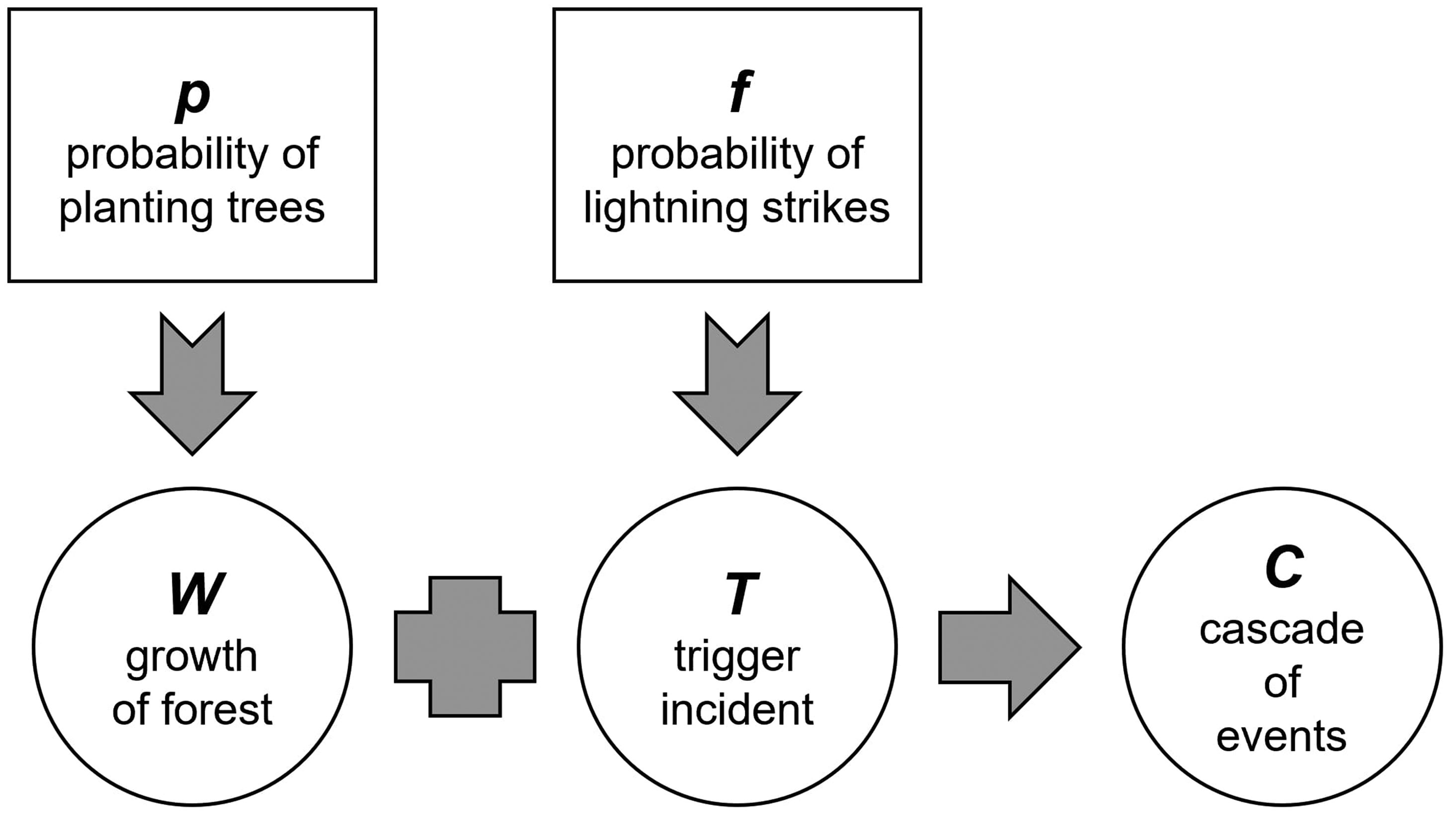
Figure 3 depicts typical examples of a PL (to the left, p-value 0.88) and of an SE (to the right, p-value 0.79). All relevant parameters of the classification procedure and the log–log plots of the fitted distributions can be found in the Online Appendices I and II (https://figshare.com/s/6454ca305cb86e45c998).
Examples of PL and SE dyads.
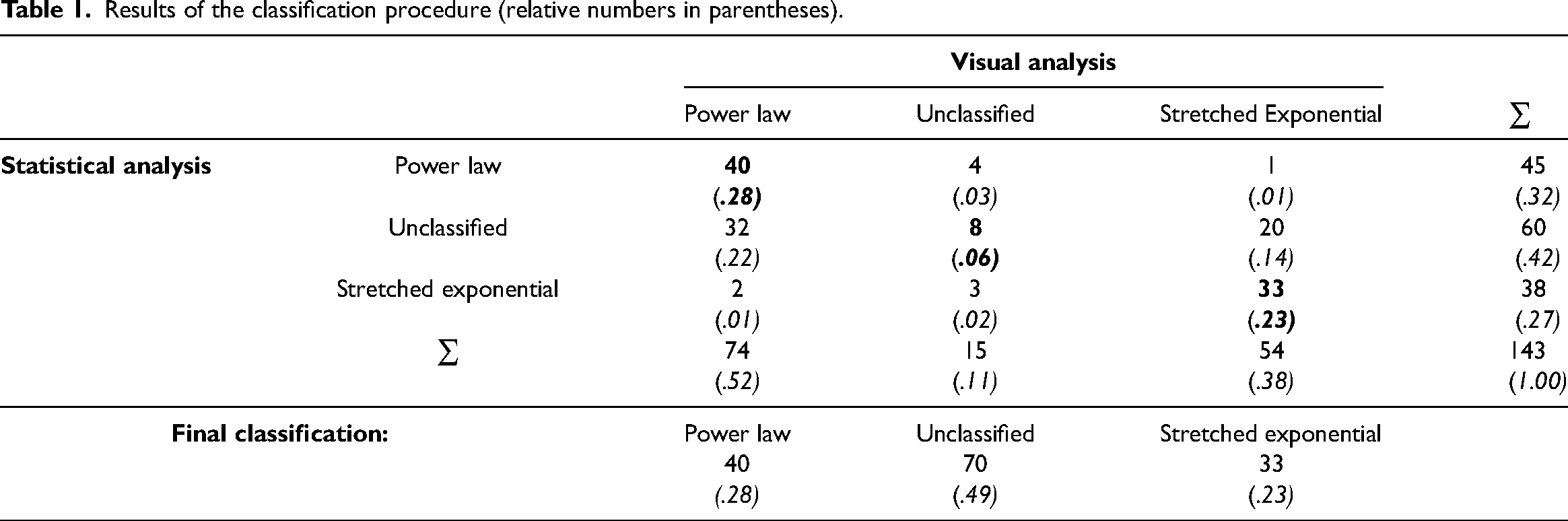
The results of the analysis are shown in Table 1. The procedure appears to be sufficiently robust: in only three cases does the visual assessment suggest a classification that directly opposes the result of the statistical analysis. The statistical analysis is pronouncedly more conservative than the visual analysis, with 83.9% of ambiguous cases being caused by statistically unclassified but visually classified cases. This indicates that human analysts are easily biased towards identifying one of the investigated distributional classes.
Results of the classification procedure (relative numbers in parentheses).
Results of the classification procedure (relative numbers in parentheses).
Despite the conservative nature of the classification procedure, 51.1% of all dyads are unambiguously allocated to one of the two categories: we identify 40 PLs and 33 SEs. Seventy dyads remain unclassified. This confirms our assumption that intrastate violent conflicts can fit other distributions than a PL. SEs are, in fact, about equally likely. Overall, eight of the classified dyads had cutoffs.
Figure 4 illustrates the distribution of the minimum event size xmin for all clearly allocated dyads on a logarithmic scale. There are both PL and SE cases where the data follows the respective distribution over the whole range (xmin = 1). About half of the PL distributions start at between three and 11 fatalities. About half of SE cases begin at between two and seven fatalities. There are no outliers.
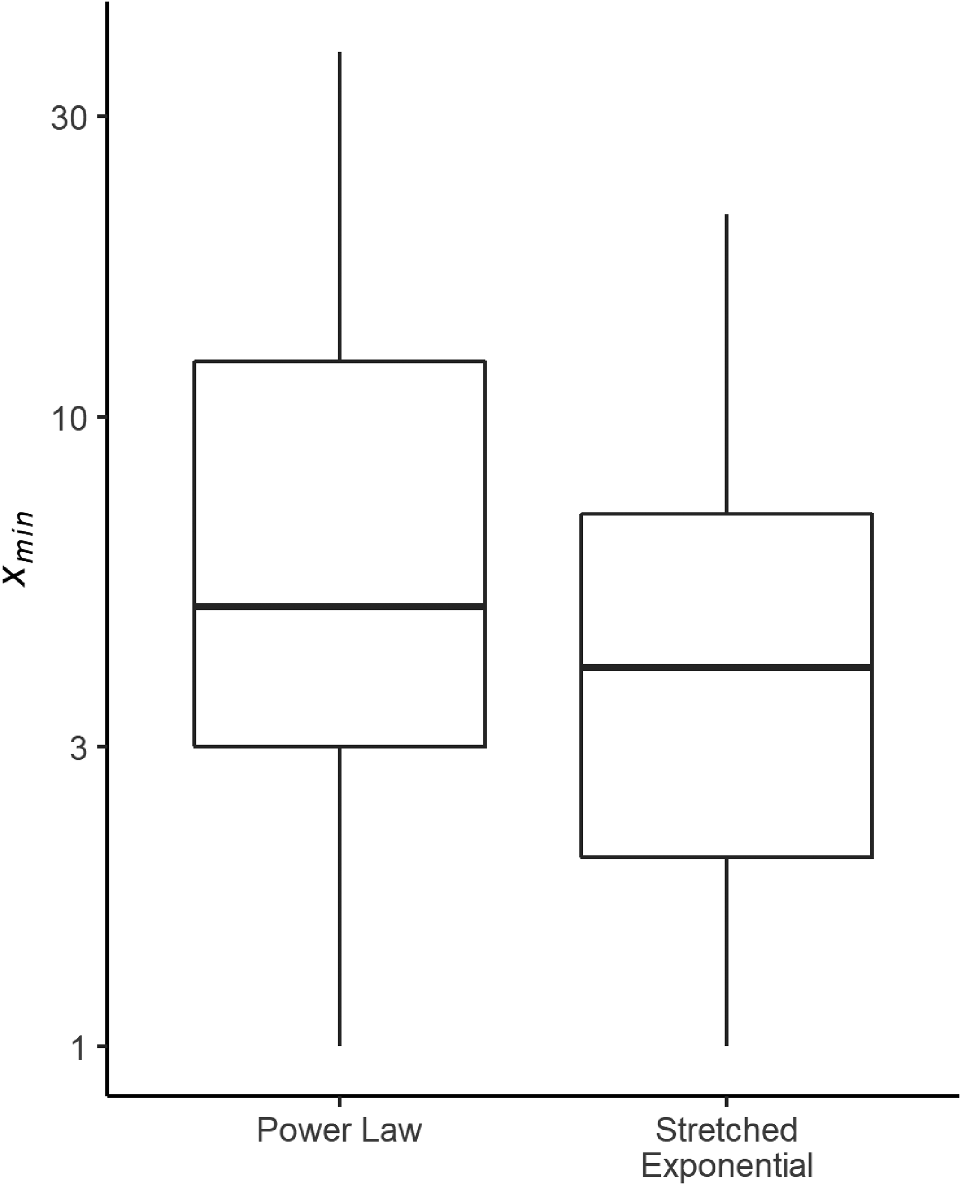
Boxplots of xmin values over distribution types on a logarithmic scale.
The literature suggests that estimated PL coefficients of intrastate intensity distributions cluster around a value of 2.5 (Bohorquez et al. 2009; Trinn 2015; Spagat et al. 2018). Most of the PL cases in our sample exhibit an exponent α between 2 and 2.5, with a median of 2.27 (Figure 5). This is close to Richardson's original findings: 1.5 for wars, 2.38 for small wars, 2.29 for banditry in Manchukuo, and 2.30 for gang violence in Chicago (Richardson 1948).
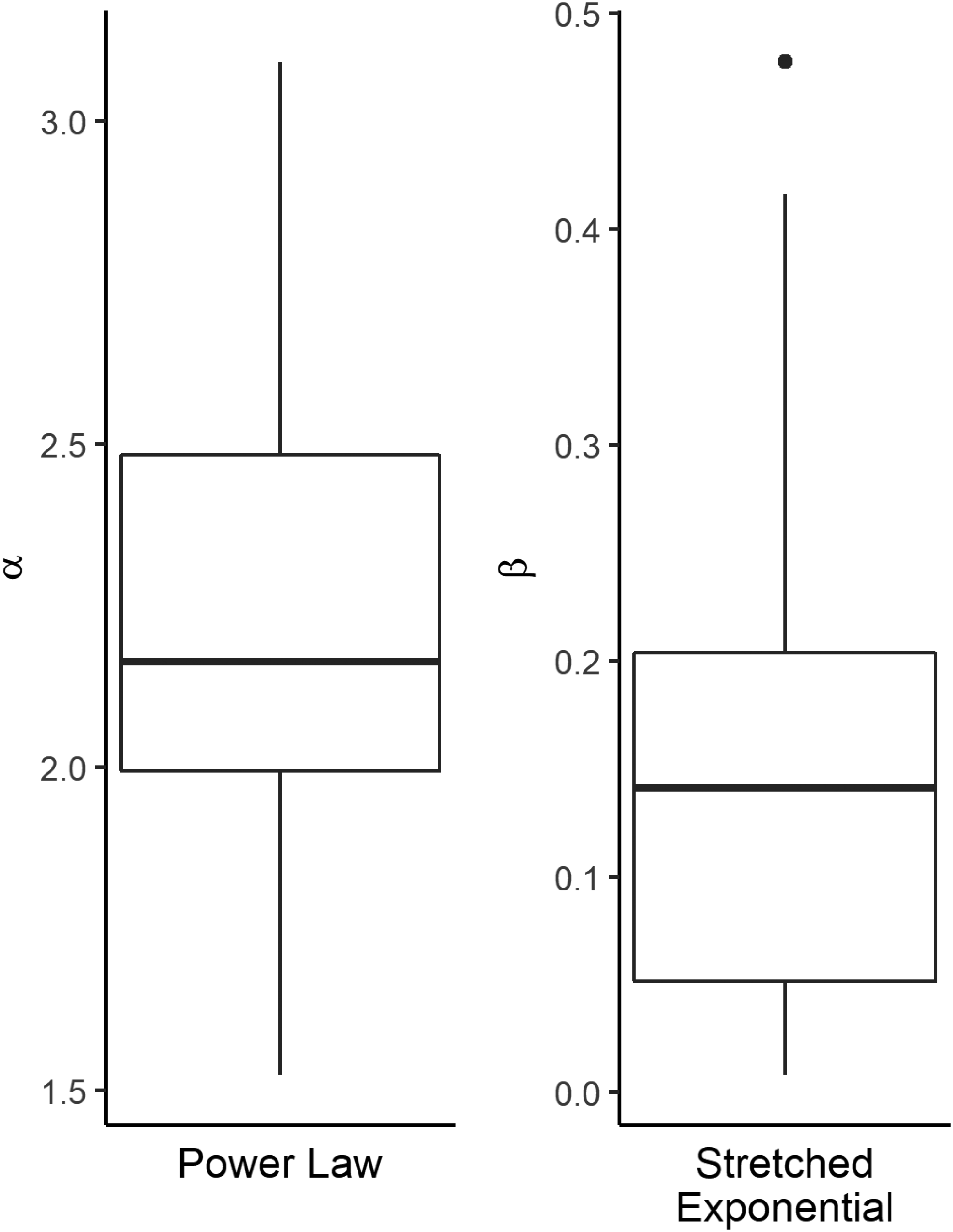
Boxplots of distribution parameters.
For all classification categories, Figure 6 depicts the total number of violent events per dyad and the number of total fatalities per dyad on a logarithmic scale, yielding no significant difference. Some 90% of unambiguously classified cases have a total number of violent events of above 51.8, while 90% have a total fatality count of above 324.4. We could use this a rule of thumb for future research: only when the number of violent events exceeds 50, or when the total number of fatalities exceeds 300, can we justifiably expect to identify either a PL or an SE distribution. For both event and fatality counts, the existence of outliers is not surprising, but rather inherent to PL and SE distributions (see the theoretical discussion).
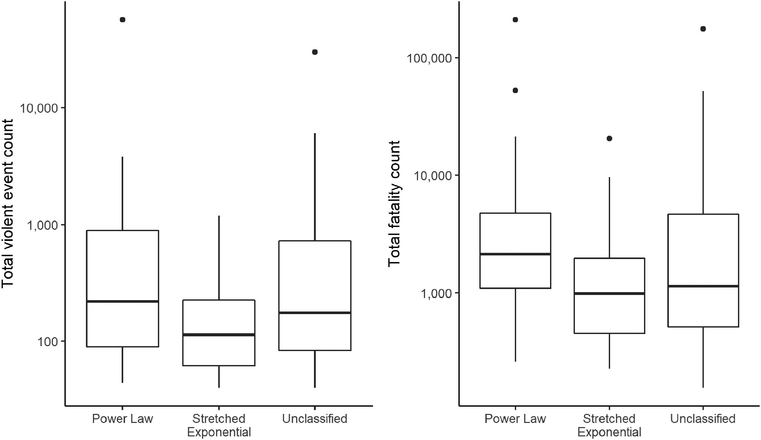
Boxplots of violent event counts and fatality counts over classification categories on a logarithmic scale.
As a result of our classification method being conservative, about half of the investigated dyads were not classified unambiguously. To avoid the risk of omitting cases that would actually be identifiable, we will now take a closer look at the 70 unclassified cases.
A simple explanation for not being able to classify a conflict dyad would be a lack of data. While we from the start excluded dyads with extremely low n for both events and unique event sizes, these restrictions might still have been too soft. Figure 7 therefore compares the distributions of these two statistics for classified and unclassified cases separately. They are very similar, even to the point that there is both a classified and an unclassified positive outlier for the number of events. This similarity rules out the explanation that many dyads were unclassified owing to a lack of data.
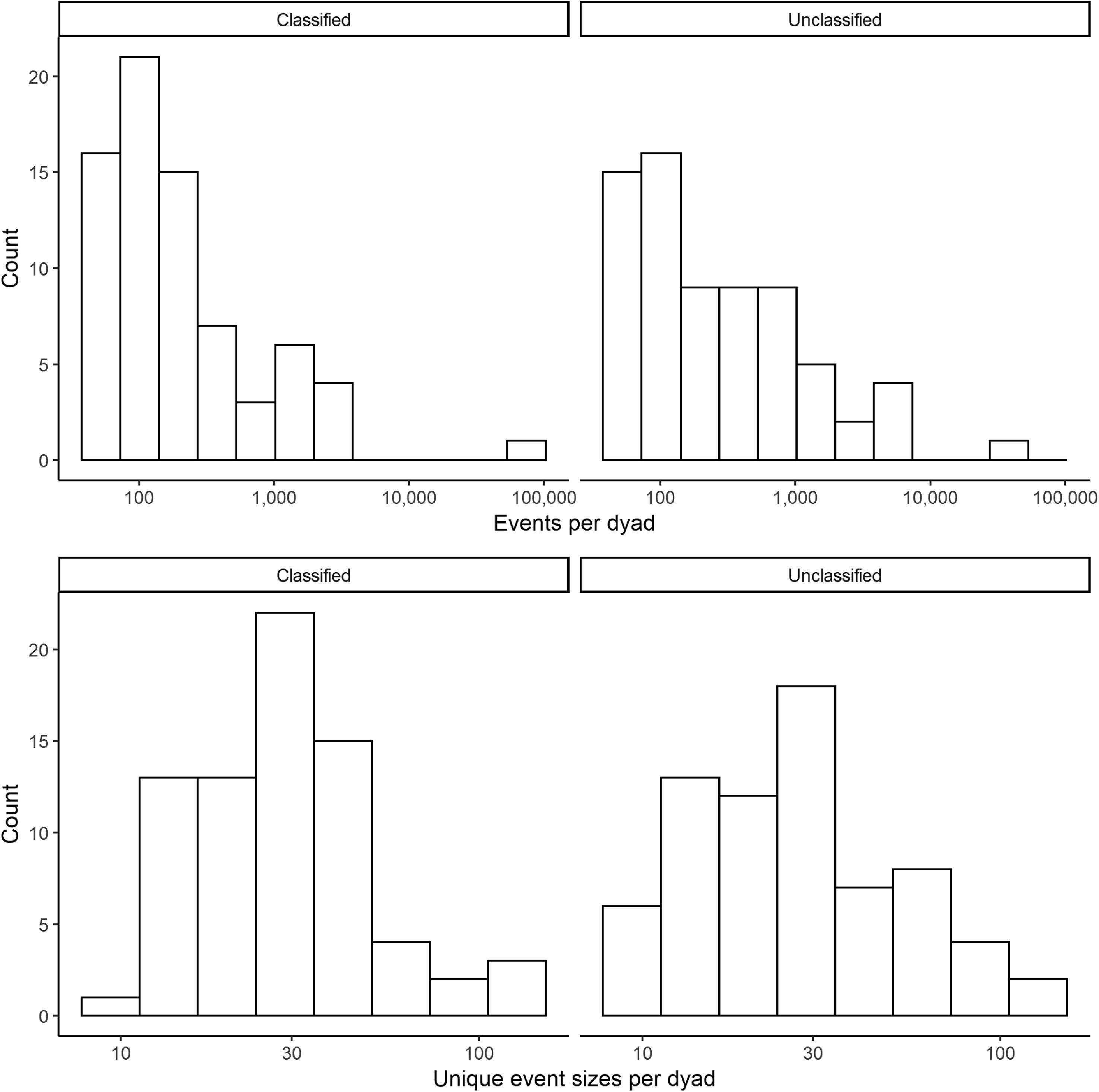
Histograms of number of events and unique event sizes per dyad on a logarithmic scale.
To go into even more detail, we divided the unclassified cases into four categories based on the statistical analysis, as this step is decisive for most unclassified cases (60 out of 70 cases): (1) direct contradictions between algorithm and human classification (three cases); (2) dyads where, in general, both distribution classes are plausible for the algorithm (pPL > 0.1 and pSE > 0.1, six cases); (3) dyads where no distribution class is plausible (pPL ≤ 0.1 and pSE ≤ 0.1, 35 cases); or (4) dyads where only one distribution class is possible, but that class is not significantly better than the other (pcomp > 0.1, 19 cases). Figure 8 depicts three randomly drawn examples for all four categories of unclassified cases, for direct contradictions this is already the whole population. It can be seen that, also for the human eye, the classification of these dyads is ambiguous. A notable exception is Government of Afghanistan—Taleban, which a human coder would naively classify as PL. However, having a pPL value of 0.00, the human eye is clearly at fault here.
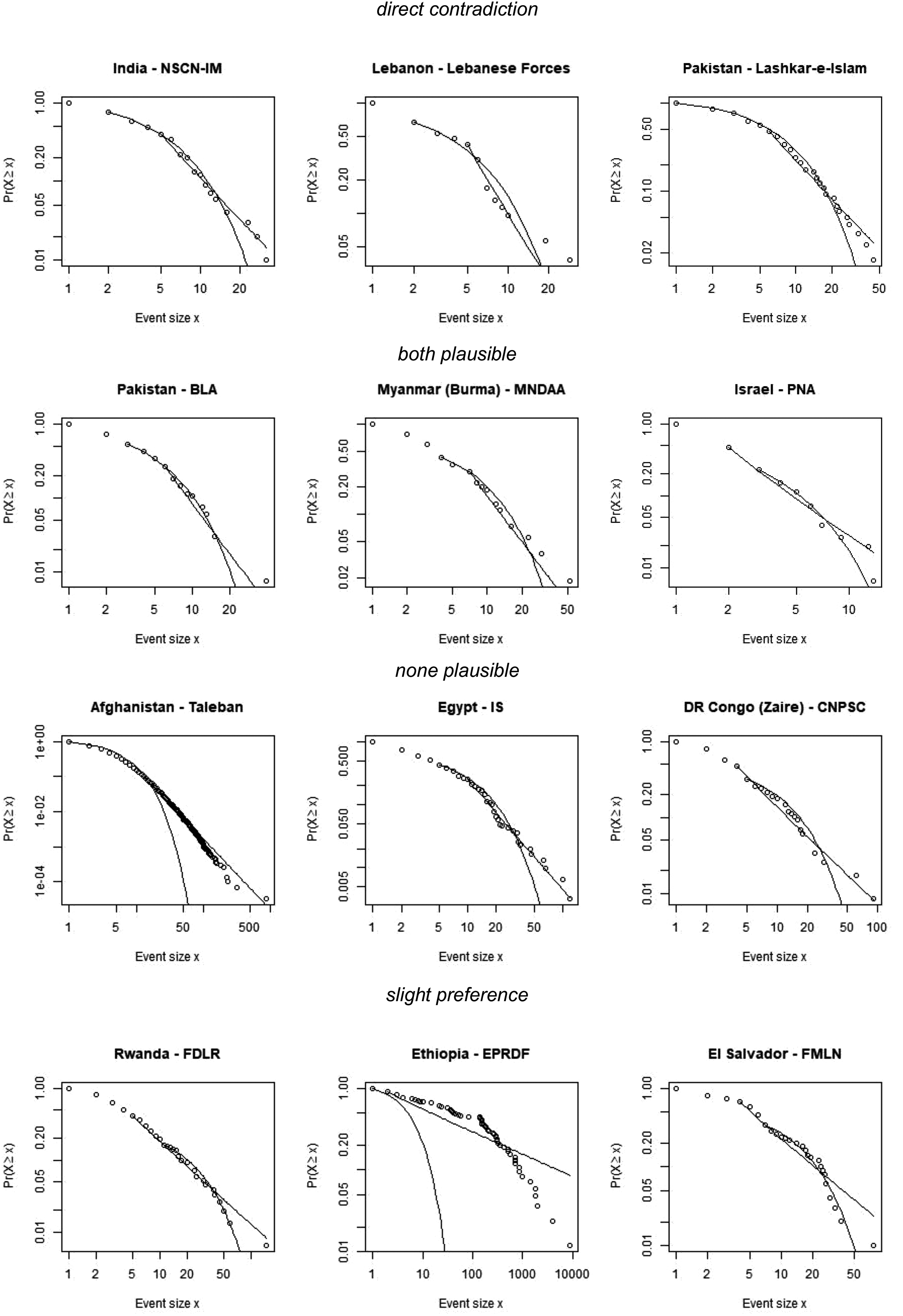
Random examples of all four categories of unclassified cases.
Thus, the considerable share of unclassified cases is not due to a lack of observations, but rather due to dyads that are ambiguous to both humans and machines. Our classification procedure is therefore conservative, but intentionally so. The ambiguity of cases might arise either from poor data quality or from alternative data generating distribution types.
The forest-fire model discussed in Section 3.2 exploits the combined variation of the parameters f and p in predicting the outcome (PL or SE event size distributions). In Section 3.3 we specified f as the density of social interactions between conflict parties and p as the grievance experienced by social groups. These are our central explanatory variables.
In state-based conflicts, the probability of interaction between the conflict actors is largely a function of the ability of the non-state group to keep its distance from the government. In turn, this depends on both the capacities of the state and the strength of the non-state actor. In asymmetrical conflicts, the non-state groups stand no chance against state intervention. This contrasts with symmetrical scenarios, where a strong rebel group confronts a relatively weak government. While asymmetric conflicts provide ample opportunities for the occurrence of triggering events, symmetrical scenarios reduce the interaction density in the dyad.
We measure state capacity as the government's potential for repression. This is proxied by the state's military expenditure per capita. We used World Bank data to calculate the median military expenditure in current US dollars and the median population size over the course of each dyad's conflict. Start and end years of conflicts were taken from the GED. Cases with fewer than one-third of the conflict years covered by data were excluded. Governments above the sample median can be considered as relatively strong. Owing to data availability, this measure is superior to other possible measures of state capacity, such as taxation as percentage of the gross domestic product. All relevant information on this and the other indicators can be found in the Online Appendix III (https://figshare.com/s/6454ca305cb86e45c998).
We argue that the ability of a non-state group to isolate itself from the rest of society is best captured by the concept of non-state governance (Mampilly 2011; Huang 2016). It describes a non-state conflict actor that exerts territorial control and also exhibits efforts to rule. Territorial control refers to the capability of a non-state group to organize at least partially effective control over a territory and its population, which is a prerequisite for the extraction of resources and thus for the group's political and military survival. Territorial control does not always mean exclusive and undisputed command over contiguous swathes of land. Armed conflicts frequently fracture the political geography into a checkerboard of zones under different rulers, while in other cases state and non-state actors compete for control over the same disputed area (Arjona 2014). However, “in order to ensure their viability, insurgent leaders cannot only be concerned with the establishment of a coercive apparatus (domination) but must also gain a degree of consent from the civilian population (hegemony)” (Mampilly 2011: 8). Some non-state organizations therefore move beyond strategic control and extraction. They show efforts to build a genuine political and social order. While this order might be fluid and fragile, it rests on a reciprocal process between non-state actors and civilians: a “social contract” (Arjona 2014; Kasfir 2015). Efforts to rule typically manifest in building at least rudimentary institutions that attempt to regulate private conduct and economic activities. Territorial control and the effort to rule are therefore both necessary attributes of non-state governance.
No dataset on governing and non-governing non-state actors exists that is suitable for our purpose. Huang (2016) covers only a third of our cases. We therefore conducted single-focus qualitative studies of non-state governance in the conflicts under investigation. On the one hand, we relied on the information on territorial control by non-state actors as provided by Cunningham et al. (2013). On the other hand, we extracted news reports from the LexisNexis database and Google News to assess the group's efforts to rule. We coded the maximum amount of governance a non-state actor exerted in a given conflict, blinding out the outcome (PL or SE) in the process.
We find that out of 60 clearly classified conflict dyads available for causal analysis, 21 involved a governing non-state actor. Among them are prominent examples such as the Communist Party of Nepal (Maoist) (CPN-M), Hamas in Gaza, Hezbollah in Lebanon, the Liberation Tigers of Tamil Eelam (LTTE) in Sri Lanka, the National Union for the Total Independence of Angola (UNITA), and the Sudan People's Liberation Movement/Army (SPLM/A). Some entities of non-state governance have evolved into officially recognized subnational political units (Autonomous Region of Bougainville in Papua New Guinea) or into fully or partially recognized states (Croatia, South Sudan) or gained national governing power (in the case of the CPN-M). Most entities, however, have remained unrecognized, retained a tenuous position, or dissolved.
We argue that non-state governance is a better proxy of the strength of non-state actors, and thus their ability to isolate themselves from the rest of society, than the relative strength of rebel groups measured by the number of fighters or soldiers alone. 2 Furthermore, non-state governance is not dependent on state capacity. There are several cases where rebel rule exists in spite of a strong government. We argue that state capacity is not an alternative to non-state governance but a complementary factor. The power relationship and interaction patterns between conflict actors do not depend on either the state or the non-state actor alone but on both in conjunction. In order to capture the relative strength of states and rebels, we have therefore included both state capacity and non-state governance in our empirical analysis.
In conjunction, state capacity and non-state governance thus provide a measure of interaction density (f). We argue that conflicts where a relatively strong government is confronted with a ruling non-state actor are characterized by the lowest interaction density. Rebel groups that maintain territorial control and are able to regulate the social order to a significant degree despite high state capacity can largely exempt themselves from unwanted government intervention. For non-governing organizations located in a strong state the opposite is true. Between these extremes, conflicts within a weak state are associated with a fairly low interaction density if the government is faced with ruling rebels but with a higher probability of interaction if a non-governing organization is involved.
In accordance with a large body of literature, we measure grievances (p) by means of horizontal inequality (Østby 2008; Cederman et al. 2011b; Cederman et al. 2013). While a mismatch is possible between perceived and objective grievances, if a social group is significantly disadvantaged or advantaged in comparison with the rest of the country's population, it is likely that a sense of being treated unfairly arises. In our analysis we focus on economic grievances as they commonly correspond to unequal political and social access as well.
Using zonal statistics in a geographic information framework, we operationalized horizontal inequality by comparing the economic development in a conflict area with a nation's overall development. Conflict areas were constructed by creating buffers with a radius of 100 km around each conflict event and merging them into one polygon. Wealth was proxied by gridded gross domestic product estimates based on nightlight data provided by the National Oceanic and Atmospheric Administration (Ghosh et al. 2010). Satellite luminosity data is an innovative proxy for measuring subnational economic activity, for countries with low-quality statistical systems (Chen and Nordhaus 2011; Bruederle and Hodler 2018). Based on this, we calculated the mean income per capita of each conflict area and of each country. As grievances may cut both ways, with frustration to be expected in poor and rich regions relative to the country mean, we opted for a symmetrical measure of horizontal inequality between the conflict area and the country at large by applying the following formula (Cederman et al. 2011b):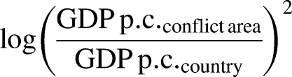
Empirical test of the theoretical expectations
With 60 cases available for causal investigation, the number of cases is limited. We therefore turn to the evaluation of binary classifiers, a method which measures the performance of a binary classifier (also called a predictor) in reproducing the allocation of cases to two outcome classes. In the present context, PL and SE constitute the outcome classes.
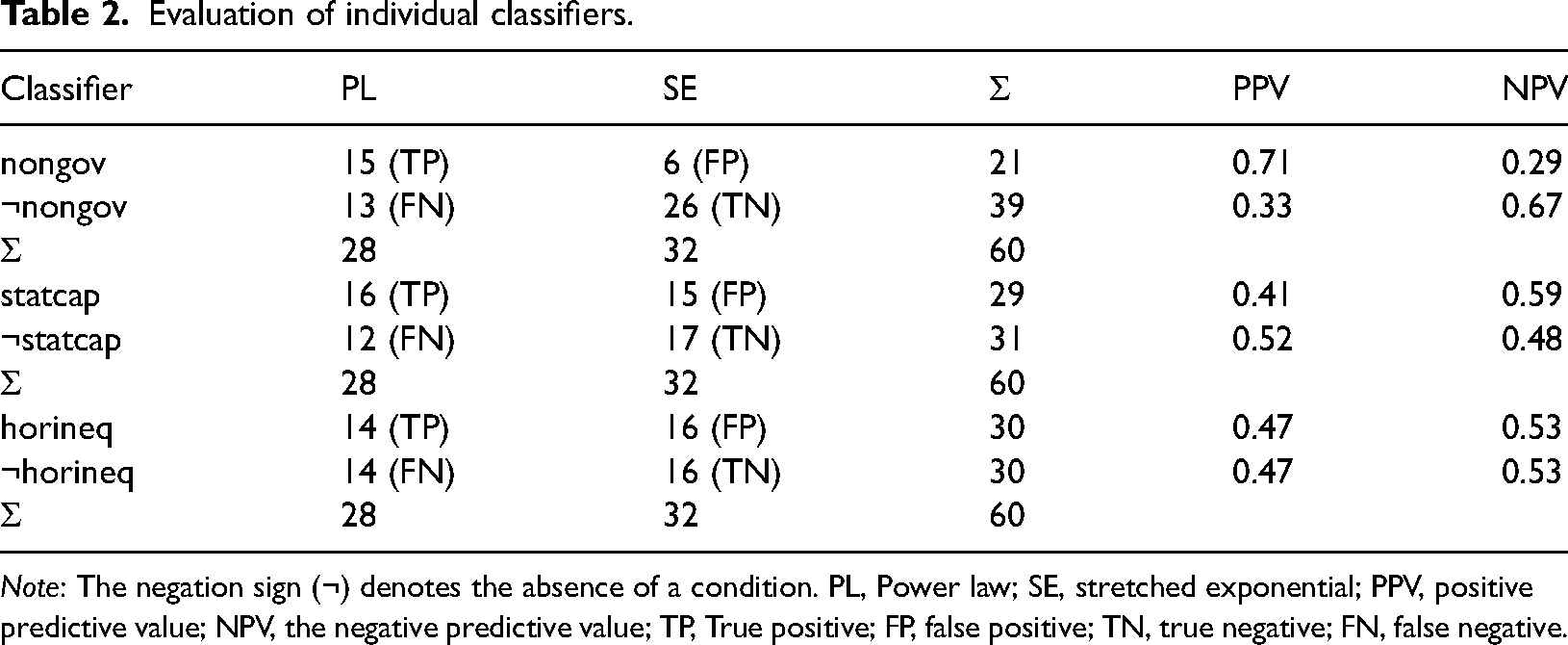
We begin by evaluating the three classifiers individually: non-state governance (nongov), state capacity (statcap), and horizontal inequality (horineq). Table 2 shows three contingency tables, giving the number of dyads that are correctly classified as PL (true positives, TP) and as SE (true negatives, TN) and the dyads falsely classified as PL (false positives, FP) or as SE (false negatives, FN). We base the evaluation of the classifiers on the positive predictive value (PPV) for PL and, inversely, the negative predictive value (NPV) for SE: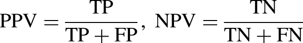
Evaluation of individual classifiers.
Evaluation of individual classifiers.
Note: The negation sign (¬) denotes the absence of a condition. PL, Power law; SE, stretched exponential; PPV, positive predictive value; NPV, the negative predictive value; TP, True positive; FP, false positive; TN, true negative; FN, false negative.
The metric, which ranges from 0 to 1, measures the “consistency” of the classifier by telling us which share of cases subjected to a condition, or combination of conditions, shows the expected outcome. We adopt a threshold of 0.6 to deem a classifier as at least fairly consistent.
Table 2 summarizes the evaluation of the three individual classifiers. The presence of non-state governance is, as expected, associated with PL distributions while the absence of ruling rebels appears to make SEs more likely. In contrast, state capacity and horizontal inequality on their own do not successfully discriminate between the two outcome classes.
By combining the three condition variables through a logical AND, we derive eight configurations. Based on our hypotheses, each of these configurations is associated with a theoretically expected outcome (dominance of PL or SE, or equal probability of both). Table 3 gives the expected outcome for each configuration of the interaction density variables (state capacity and non-state governance) and the grievance variable (horizontal inequality). It also summarizes the results of the evaluation, with each configuration functioning as a binary classifier. PL and SE event distributions are associated with the expected configurations. More specifically, we derive three main findings.
Evaluation of configurations derived from the forest-fire model.
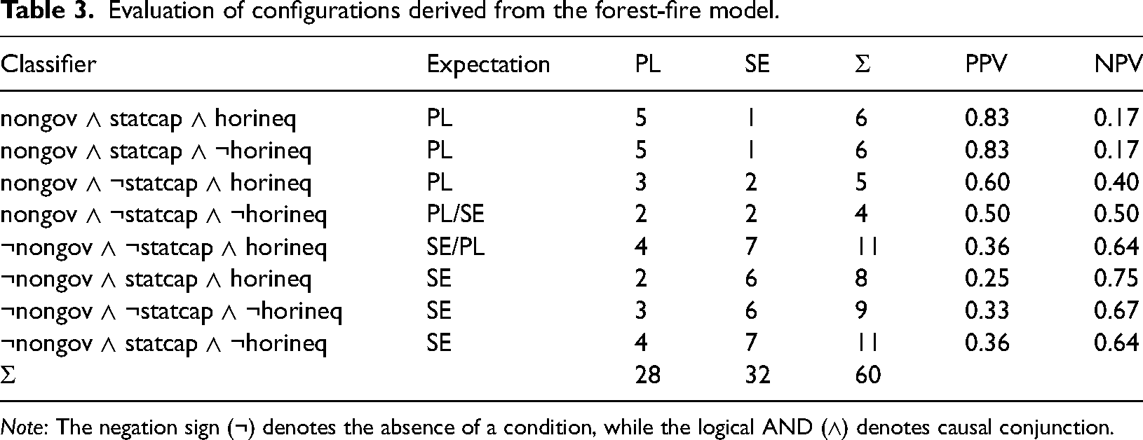
Note: The negation sign (¬) denotes the absence of a condition, while the logical AND (∧) denotes causal conjunction.
First, PLs are prevalent either where governing non-state actors coincide with a strong state, regardless of the level of grievances, or where ruling rebels encounter a weak state and widespread horizontal inequalities. With 83%, PLs are particularly dominant where the ratio of f/p is especially low, as predicted by the forest-fire model.
Second, SEs are prevalent either where “ordinary”, non-governing rebels are found in an environment characterized by low horizontal inequalities, irrespective of the state's capacity level, or where non-governing non-state actors coincide with a strong state and widespread grievances.
Third, there are indications that PLs and SEs are indeed equally likely if f and p are balanced. This is noticeable where governing insurgents confront a weak state, but where grievances prevail. This is not true for the inverse configuration, however: as SEs dominate here, our expectations are not met.
Overall, the classifiers derived from the forest-fire model perform well. Out of eight configurations, only one shows an unexpected ratio of PLs and SEs. Our empirical findings thus speak in favour of the validity of the theoretical model.
This article has sought to shed light on the “enduring mystery” of PLs in intrastate conflicts. While some researchers find nothing mysterious about the origins of PL distributed conflict intensities, explaining them away as spurious facts resulting from random fluctuations, others see them as a hallmark of complex systems: self-organizing networks where non-linear dynamics give rise to spontaneous bursts of disruptions triggered by infinitesimal incidents. Much of the debate has been theoretical, frequently relying on simulations. Empirical tests of the mechanistic assumptions of complex system models have been virtually non-existent. This article addressed this gap by evaluating the theoretical plausibility of the widely used forest-fire model and by testing its empirical validity in the context of violent intrastate conflicts.
As with all complexity models, there is a considerable gap between abstract specifications and real-world concepts. We have sought to close this gap between model and reality by offering a discussion of the model's defining components: the activation parameter, which captures the triggering of propagating activity avalanches, and the storage parameter, which represents a pre-existent, accumulating potential. We suggested that the activation parameter can be conceptualized as the likelihood that the conflict adversaries interact. We operationalized this concept by taking into account the relative strength of the state and non-state actors. We discussed the storage parameter in terms of grievances resulting from group-based comparisons, measuring this through horizontal inequalities on a disaggregated level.
The validity of the model was tested on conflict intensity event data arising from a sample of 143 state-based conflict dyads between 1989 and 2020. Our rigorous and conservative approach resulted in an unequivocal classification of about half of the dyads. Most remaining cases are empirically ambiguous, owing to either quality issues of the data basis or alternative distribution types not included in the analysis. Nevertheless, we identified 40 PL cases and 33 cases of SEs. We thus find that the two outcome distributions predicted by the model appear in the conflict event data.
A hypothesis test based on a systematic evaluation of configurational binary classifiers found that the forest-fire model is a good approximation of the dynamics of violent intrastate conflicts. Owing to the limited number of cases in our analysis, this finding is tentative. Nevertheless, it lends support to the argument that non-linear self-organizing processes indeed drive the dynamics of intrastate conflicts. This should spur quantitative as well as qualitative research into the role of triggering events in conflict escalation dynamics.
Our analysis aimed at testing the mechanistic assumptions of the forest-fire model. By targeting strategic variables, we were able to identify far-reaching theoretical implications. Our findings speak in favour of the forest-fire model, in particular, and for SOC models with their emphasis on non-linear dynamics, in general. While the complexity paradigm has been underrepresented in conflict studies so far, our findings suggest that the complex systems approach to violent political conflict is a plausible option. The debate about the role of complexity vs. randomness is far from over.
Supplemental Material
sj-xlsx-1-cmp-10.1177_07388942221092126 - Supplemental material for Guns and lightning: Power law distributions in intrastate conflict intensity dynamics
Supplemental material, sj-xlsx-1-cmp-10.1177_07388942221092126 for Guns and lightning: Power law distributions in intrastate conflict intensity dynamics by Christoph Trinn and Lennard Naumann in Conflict Management and Peace Science
Supplemental Material
sj-zip-2-cmp-10.1177_07388942221092126 - Supplemental material for Guns and lightning: Power law distributions in intrastate conflict intensity dynamics
Supplemental material, sj-zip-2-cmp-10.1177_07388942221092126 for Guns and lightning: Power law distributions in intrastate conflict intensity dynamics by Christoph Trinn and Lennard Naumann in Conflict Management and Peace Science
Supplemental Material
sj-xlsx-3-cmp-10.1177_07388942221092126 - Supplemental material for Guns and lightning: Power law distributions in intrastate conflict intensity dynamics
Supplemental material, sj-xlsx-3-cmp-10.1177_07388942221092126 for Guns and lightning: Power law distributions in intrastate conflict intensity dynamics by Christoph Trinn and Lennard Naumann in Conflict Management and Peace Science
Footnotes
Declaration of conflicting interests
The authors declared no potential conflicts of interest with respect to the research, authorship, and/or publication of this article.
Funding
The authors received no financial support for the research, authorship, and/or publication of this article.
Supplemental material
Supplemental material for this article is available online.
Notes
References
Supplementary Material
Please find the following supplemental material available below.
For Open Access articles published under a Creative Commons License, all supplemental material carries the same license as the article it is associated with.
For non-Open Access articles published, all supplemental material carries a non-exclusive license, and permission requests for re-use of supplemental material or any part of supplemental material shall be sent directly to the copyright owner as specified in the copyright notice associated with the article.